Controlling ISR in sparticle mass reconstruction

Abstract:

Use of inclusive $M_{T2}$ distribution for sparticle mass determination is discussed. We define new parameters $M_{T2}({\rm min})$ and $M_{T2}^{\rm mod}({\rm min})$, which are a kind of minimum of sub-systerm $M_{T2}$ values. Their endpoints are less affected by initial state radiations. We demonstrate that both $m_{\tilde{q}}$ and $m_{\tilde{g}}$ can be extracted from the endpoints of the distributions in the wide region of parameter space expected in CMSSM. We also present a comparison with $M_{TGen}$ distributions.

1 Introduction

The quest of physics beyond the standard model is now reaching new phase with the LHC experiments[1, 2] and various new dark matter (DM) searches[3, 4]. In models with conserved parity for stability of a dark matter, new coloured particles may be produced in pairs at the LHC and each of them decays into particles involving the stable dark matter. This gives missing transverse momentum to the events, which would be useful in separating the signal from QCD backgrounds. Especially, in supersymmetric (SUSY) models squarks and gluino are produced and decay into lighter particles involving the lightest SUSY particle (LSP) which is usually identified as the dark matter. The signature is events with jets (+leptons) + missing transverse momentum.

Because the dark matter cannot be detected in the LHC detectors, masses of SUSY particles cannot be reconstructed as resonances. Various techniques to determine the masses of SUSY particles have been studied (See Ref.[5] for a recent review.). Important kinematical variables are peak position of $M_{\rm eff}$ distribution, the endpoints of invariant mass distributions of jets and leptons[6, 7, 8, 9, 10, 11, 12, 13, 14, 15], the endpoint of $M_{T2}$ distributions[16, 17, 18, 19, 20, 21, 22, 23, 24, 25, 26, 27, 28, 29, 30]. Among those, most clean channel is probably the invariant mass distributions of $jll$ channel although the branching ratio of this mode is rather small.

In the early stage of the LHC, it is more useful to study the distribution with jet + $E_{Tmiss}$ channel[23, 24]. The number of signal events is rather small in the discovery phase, therefore if we require multiple leptons in the final state, we would not be able to obtain an event sample large enough to do analysis. For this problem, quantities that are less sensitive to the detail of the decay pattern are useful.

In previous papers[23, 24], we have defined an inclusive $M_{T2}$, which is calculated for any SUSY events at the LHC using hermisphere method. Hemisphere method is the way to define two sets of particles in the event, and each set (called hemisphere) contains particles coming from the same parent particle decay in the limit that parent sparticles are highly boosted into back-to-back[31, 32]. We have shown an interesting correlation between the endpoint of the inclusive $M_{T2}$ distribution and mass of the heavier of squark and gluino. We have also demonstrated that a subsystem $M_{T2}$, $M_{T2}({\rm sub})$, is useful to determine the gluino mass for $m_{\tilde{g}}<m_{\tilde{q}}$ case[24].

One of the important issues for mass reconstruction is existence of initial state radiation (ISR)[26, 33, 34, 35, 36]. When we produce heavy particles at the LHC, there would be a hard ISR jet which could have $p_{T}$ about the same order of the mass of the produced particle. The ISR jets may be involved among the jets for the invariant mass or $M_{T2}$ calculations, then the distributions are smeared. In Ref.[26], it is shown that the effect of leading ISR can be removed by minimizing “$M_{T2}$ after removing a jet” for several choices of a removing jet. Smearing due to ISR is significantly reduced by this procedure for a limited example $\tilde{g}\tilde{g}$ production process followed by $\tilde{g}\rightarrow\tilde{\chi}^{0}_{1}jj$.

In this paper we define a $M_{T2}({\rm min})$ to reconstruct the endpoint of $M_{T2}$ distribution under the effect of ISR for general squark and gluino production processes. The definition is also consistent with the previously defined $M_{T2}({\rm sub})$ to obtain $m_{\tilde{g}}$ when $m_{\tilde{g}}<m_{\tilde{q}}$. We extend our studies so that we can cover $m_{\tilde{q}}\leq m_{\tilde{g}}$ case as well, so that $m_{\tilde{g}}$ is reconstructed by the appropriate choice of quantities. For this purpose, we define a $M_{T2}^{\rm mod}({\rm min})$ for the events that two highest $p_{T}$ jets coming from two body decays with large mass differences between parent and daughter particles and there are two jets which are prominent over the other jets. As its nature, the $M_{T2}^{\rm mod}({\rm min})$ works for $m_{\tilde{q}}\leq m_{\tilde{g}}$. We provide parton level and jet level studies and demonstrate that these quantities are actually important.

This paper is organized as follows. In section 2, we introduce basic parameters such as $M_{T2}$ and $M_{T2}({\rm sub})$, which has been defined in the previous papers by using hemispehre algorithm, and summarize previous analyses. We also define new parameters $M_{T2}({\rm min})$, and $M_{T2}^{\rm mod}({\rm min})$. These parameters are defined to reduce ISR effects but for different squark and gluino decay patterns. Section 3 is for parton level study of hemisphere analysis, which is efficient for inclusive analysis. Section 4 describes the parton level distribution of $M_{T2}({\rm min})$ and $M_{T2}^{\rm mod}({\rm min})$ with and without ISR. The needs of $M_{T2}^{\rm mod}({\rm min})$ will be explained in this section. In section 5, we discuss jet level $M_{T2}$, $M_{T2}({\rm min})$ and $M_{T2}^{\rm mod}({\rm min})$ distributions. The measured endpoints depend on the dominant decay pattern of sparticles. We found the decay pattern can be determined from simpler quantities such as $p_{T}$ of the two highest $p_{T}$ jets and hermisphere mass distributions. The inclusive $M_{T2}$ study can be applied in the early stage of the LHC. The expected distribution at $\sqrt{S}=7$ TeV and $\int{\cal L}dt=1\,{\rm fb^{-1}}$ is shown in section 6. Section 7 is devoted for discussions and conclusions.

2 Inclusive $M_{T2}$ distribution, ISR, and mixed production

The discovery of supersymmetric particles at the CERN LHC has been studied in depth[37, 38, 39, 40, 41, 42, 43, 44, 45, 46]. In recent articles[45, 46], the discovery region at $\sqrt{s}=7$ TeV and $\int{\cal L}dt=1\,$fb^-1 in CMSSM has been studied. One can read from Fig. 13 in Ref.[46] that the region $m_{0}<850\,(750)$ GeV at $M_{1/2}<210\,(250)$ GeV can be explored, respectively. Here $m_{0}$ and $M_{1/2}$ are universal scalar and gauino masses. In Fig. 1, we show the total SUSY production cross section as a function of $m_{0}$ for $M_{1/2}=210$ (250) GeV at $\sqrt{S}=7$ TeV (left) and 14 TeV (right). The model points appeared in Fig. 1 are defined in Table 1. The cross section at each model point is calculated by HERWIG[47, 48, 49]. The cross section at the boundary of the discovery region for $\sqrt{S}=7$ TeV with $\int{\cal L}dt=1$ fb^-1 is roughly $\sigma_{SUSY}=1$ pb. After the 7 TeV run, the collision at 14 TeV is scheduled. The cross sections at 14 TeV is about 10 times larger than those at 7 TeV.

Figure 1: Total SUSY production cross sections for the model points in Table 1 as a function of $m_{0}$ for fixed gaugino masses at 7 TeV (left) and 14 TeV (right). The CMSSM points are produced by ISASUSY[50], and the cross sections are estimated by HERWIG[47, 48, 49]. The $\tilde{u}_{L}$ masses and names of the model points are also shown in the figure.

By studying production cross sections of sparticles at the LHC, patterns for sparticle masses can be investigated. The production cross section is sensitive to the mass scale of produced particles, as can be seen in Fig. 1, and it is an important piece of information on the mass scale. Increasing mass by 100 GeV leads 50 % reduction of the cross section at $m_{\tilde{g}}\sim m_{\tilde{u}_{L}}\sim 500$ GeV. The uncertainty of the squark and gluino production cross section would be less than 10 %[51].

	Point 1’	2’	3’	4’	5’
$m_{0}$(GeV)	100	200	420	550	700
$M_{1/2}$	210	210	210	210	210
$m_{\tilde{g}}$	522	528	541	550	558
$m_{\tilde{u}_{L}}$	478	508	619	708	825
$m_{\tilde{u}_{R}}$	466	496	611	702	820
$\sigma_{\rm SUSY}({\rm 14TeV})$ in pb	88.7	90.1	44.8	31.4	23.2
$\sigma_{\rm SUSY}({\rm 7TeV})$ in pb	10.9	10.8	4.59	3.12	2.60
$\sigma({\tilde{g}\tilde{q}})/\sigma_{\rm SUSY}$ at 14TeV	0.52	0.46	0.49	0.48	0.45
$\sigma({\tilde{g}\tilde{g}})/\sigma_{\rm SUSY}$ at 14TeV	0.14	0.14	0.21	0.28	0.37
$\sigma({\tilde{q}\tilde{q}})/\sigma_{\rm SUSY}$ at 14TeV	0.21	0.18	0.15	0.12	0.08
$Br(\tilde{u}_{L}\rightarrow\tilde{g})$	0	0	0.26	0.48	0.56
$Br(\tilde{u}_{R}\rightarrow\tilde{g})$	0	0	0.60	0.82	0.87

	Point 1	2	3	4	5
$m_{0}$	100	250	500	650	750
$M_{1/2}$	250	250	250	250	250
$m_{\tilde{g}}$	612	620	636	646	651
$m_{\tilde{u}_{L}}$	560	602	734	837	913
$m_{\tilde{u}_{R}}$	544	589	724	828	906
$\sigma_{\rm SUSY}({\rm 14TeV})$ in pb	38.1	30.5	17.7	12.8	10.6
$\sigma_{\rm SUSY}({\rm 7TeV})$ in pb	4.2	3.1	1.7	1.2	1.1
$\sigma({\tilde{g}\tilde{q}})/\sigma_{\rm SUSY}$ at 14TeV	0.47	0.48	0.46	0.43	0.39
$\sigma({\tilde{g}\tilde{g}})/\sigma_{\rm SUSY}$ at 14TeV	0.11	0.12	0.18	0.22	0.25
$\sigma({\tilde{q}\tilde{q}})/\sigma_{\rm SUSY}$ at 14TeV	0.22	0.21	0.16	0.12	0.0 9
$Br(\tilde{u}_{L}\rightarrow\tilde{g})$	0	0	0.249	0.469	0.611
$Br(\tilde{u}_{R}\rightarrow\tilde{g})$	0	0	0.582	0.813	0.891

Table 1: Masses and important branching ratios in some CMSSM points. Points 1 $-$ 5 for fixed gaugino mass $M_{1/2}=250$ GeV, Points 1’ $-$ 5’ for $M_{1/2}=210$ GeV. Mass spectrum are calculated by ISASUSY[50] and cross sections are calculated by HERWIG[47, 48, 49].

One can determine the mass spectrum directly from kinematical distributions of sparticle decay products. If both squark and gluino masses can be determined, one can further study their interaction by comparing the measured production cross section with the theoretical value, because the dependence on the other parameters are rather small[52, 53].

In SUSY models with conserved R parity, two LSPs escape from detection for each SUSY event, therefore masses of sparticles cannot be measured as resonances. (In this paper the LSP is assumed to be the lightest neutralino, $\tilde{\chi}_{1}^{0}$.) Endpoints of invariant mass distributions of jets and leptons distribution can be used to determine the masses. For example in $\tilde{q}\rightarrow\tilde{\chi}^{0}_{2}\rightarrow\tilde{l}\rightarrow\chi^{0}_{1}$ produce a $jll$ final state and endpoints of the invaiant mass distribution $m_{jll}$, $m_{jl}(min)$, $m_{jl}(max)$, $m_{ll}$ can be used to determine the all sparticles masses involved in the decay. However, branching ratios of favorable modes such as $jll$ are generally small, and they may not be useful in the early stage of the experiments. Therefore it is important to find inclusive quantities sensitive to squark and gluino masses so that one can use the most of the signal events at the LHC.

Typical energy scale of sparticle production processes may be estimated from the “effective mass”,

$$M_{\rm eff}\equiv\sum_{i}|p_{Ti}|+E_{T}^{\rm miss}\,,$$ (1)

where in this paper the sum is taken for the jets with $p_{T}>50$ GeV and $\eta<$2.5. A peak value of the $M_{\rm eff}$ distribution is correlated with squark and gluino masses, although the relation is rather qualitative[54].

More recently, we have proposed an “inclusive $M_{T2}$” which is calculated from jet (and lepton) momenta and the missing transverse momentum[23, 24]. The definition of $M_{T2}$ is the following[16, 17]:

$$M_{T2}\equiv\min_{p^{\chi}_{T1}+p^{\chi}_{T2}=p_{T}^{\rm miss}}\left[\max\left(M_{T}(p_{v_{1}},p_{1}^{\chi}),M_{T}(p_{v_{2}},p_{2}^{\chi})\right)\right].$$ (2)

Here $v_{1}$ and $v_{2}$ are two selected visible systems in an event, and $p^{\chi}_{i}$ is a test LSP momentum with a test mass $m_{\chi}$. If $v_{1}$ and $v_{2}$ arise from two on-shell particles $A_{1}$ and $A_{2}$ as $A_{i}\rightarrow v_{i}\chi^{0}_{1}$, respectively, the $M_{T2}$ is bounded from above as

$$M_{T2}\leq\max(m_{A_{1}},m_{A_{2}})~{}~{}~{}{\rm for}~{}m_{\chi}=m_{\chi^{0}_{1}}$$ (3)

by its construction. Therefore by measuring the endpoint of $M_{T2}$ distribution, one can measure the mass of the heavier of parent particles. Moreover, the LSP mass can be determined by measuring a kink position of the $M_{T2}^{\rm max}(m_{\chi})$ as a function of the test mass $m_{\chi}$[19, 21, 22]. Throughout this paper, we fix $m_{\chi}=m_{\tilde{\chi}_{1}^{0}}$ for simplicity.

To determine masses of squark or gluino from the $M_{T2}$ endpoint, decay products of sparticles should be correctly identified to $v_{i}$. Unless the event has relatively simple topology such as $pp\rightarrow$$\tilde{q}\tilde{q}\rightarrow(j\tilde{\chi}^{0}_{1})(j\tilde{\chi}^{0}_{1})$ or $pp\rightarrow\tilde{g}\tilde{g}$$\rightarrow$ $(jj\chi^{0}_{1})(jj\chi^{0}_{1})$, some of the jets are mis-grouped into wrong $v_{i}$. It has been proposed in[31, 32] hemisphere algorithm is useful to define $v_{i}$. It is defined as follows;

1. Take two jets as the first seeds of the two hemisphere $H_{1}$ and $H_{2}$, $J_{1}\in H_{1}$ and $J_{2}\in H_{2}$: $J_{1}$ is the highest $p_{T}$ jet, and $J_{2}$ is the jet ($i$) whose $p_{Ti}\times\Delta R(p(J_{1}),p(i))$ is the largest in the event.

2. Associate the other jets to the one of the hemispheres based on a distance measure $d$, so that $j_{k}$ belongs to $H_{i}(i=1,2)$ if $d(i,k)<d(j,k)$. Here $d$ is defined as

   $$d(p_{\rm hemi}^{(i)},p_{k})=(E_{\rm hemi}^{(i)}-|p_{\rm hemi}^{(i)}|\cos\theta_{ik})\frac{E^{(i)}_{\rm hemi}}{(E^{(i)}_{\rm hemi}+E_{k})^{2}}.$$ (4)

3. Take the sum of the jet momenta that belong to $H_{i}$ and regard it as a new seed. Repeat the processes 2 and 3, while keeping the first seeds $J_{1}$ and $J_{2}$ in the different hemispheres, till the assignment converges.

After defining the hemisphere, we define the inclusive $M_{T2}$ using $p_{v_{i}}=\sum_{k\in H_{i}}p_{k}$. In this paper we only use jets with $p_{T}>$50 GeV and $|\eta|<$2.5.

Alternatively, it was proposed to use $M_{TGen}$ which is the minimum of the $M_{T2}$s for all choices of jet combinations[18]

$$M_{TGen}\equiv\min_{1\leq\alpha\leq 2^{n-1}-1}M_{T2}(p_{H_{i}^{\alpha}},p_{H_{j}^{\alpha}},p_{T}^{\rm miss},m_{\chi})$$ (5)

where $\alpha$ denotes a possible combination to split jets into two groups $H_{1}^{\alpha}$ and $H_{2}^{\alpha}$, and minimization is taken over all possible $2^{n-1}-1$ combinations. Furthermore, $p_{H_{i}^{\alpha}}=\sum_{k\in H_{i}^{\alpha}}p_{k}$ and $n$ is the number of visible objects. If all jets and leptons are decay products of $A_{1}$ and $A_{2}$, $M_{TGen}\leq\max\{m_{A_{1}},m_{A_{2}}\}$.

At hadron collision, there are also particles coming from ISR in addition to those from sparticle decays. Transverse momentum of the ISR jet can be as large as those from squark and gluiino decays. The ISR jets in the visible systems $v_{1}$ and $v_{2}$ smear the $M_{T2}$ endpoint significantly.

In Ref.[26] a new definition of $M_{T2}$ that reduce ISR effect is defined, and mass determination based on the quantity is demonstrated for a $pp\rightarrow\tilde{g}\tilde{g}X$ process followed by a gluino decay $\tilde{g}\to jj\chi^{0}_{1}$, where $X$ is a ISR partons. The ISR improved $M_{T2}$, $M_{T2}({\rm min})$, is defined as follows;

1. Calculate $M_{T2}(i)$ which is a $M_{T2}$ calculated with a given grouping procedure but without involving the $i$-th jet in $p_{T}$ order. In this paper, we take hemisphere algorithm after removing the $i$-th jet for the grouping.

2. Take the minimum of the $M_{T2}(i)$ over the certain range of $i$,

   $$M_{T2}({\rm min})\equiv\min_{i}M_{T2}(i).$$ (6)

In Ref.[26], the minimization is taken up to the fifth jet and $M_{T2}$ is calculated by 4 jets because a gluino forced to decay into $jj\tilde{\chi}^{0}_{1}$. The contamination above the endpoint is significantly reduced for $M_{T2}({\rm min})$ distribution. In the paper, however, only the limited process was studied, and the techniques should be extended to the other SUSY processes, especially gluino-squark co-production because it is the dominant production process for a wide region of the parameter space (See Table 1.).

A merit to use another definition of the $M_{T2}$ for gluino-squak co-production, $M_{T2}({\rm sub})$, has been discussed in Ref.[24]. It is defined as the $M_{T2}$ but the highest $p_{T}$ jet is not included, namely,

$$M_{T2}({\rm sub})\equiv M_{T2}(1).$$ (7)

In the parameter region where $m_{\tilde{q}}>m_{\tilde{g}}$, the subtraction of the highest $p_{T}$ jet tends to reduce the full-system of $\tilde{q}$-$\tilde{g}$ into the subsytem of $\tilde{g}$-$\tilde{g}$ or $\tilde{g}$-$\tilde{\chi}_{i}$ ($\tilde{\chi}_{i}$ denotes charginos or neutralinos.) effectively because squarks either decay into $\tilde{g}$ or $\tilde{\chi}_{i}$ with high probability. In this case, we have

$$M_{T2}({\rm sub})\leq m_{\tilde{g}}.$$ (8)

It is shown that the endpoint of the $M_{T2}({\rm sub})$ correlates with gluino mass very well. By definition, $M_{T2}({\rm min})<M_{T2}({\rm sub})$, therefore the $M_{T2}({\rm min})$ distribution may improve the sensitivity to the gluino mass by reducing the tail of the distribution.

The parameter region with $m_{\tilde{q}}<m_{\tilde{g}}$ is not considered in Refs.[23, 24, 26]. For such a parameter region, gluino decays into $j\tilde{q}$, and the squark further decays into $j\tilde{\chi}_{i}$. The jet from the squark two body decay has significant energy of the order of $|p_{Tj}|\sim m_{\tilde{q}}/2$ for CMSSM like mass spectrum with $m_{\tilde{q}}\gg m_{\tilde{\chi}_{i}}$. The $p_{T}$ of the jet from the two body decay tends to be harder than that of ISR jet, therefore including the highest $p_{T}$ jet for the minimization for $M_{T2}({\rm min})$ may remove a jet from the squark decay with high probability, making the distribution near the endpoint rather flat. Therefore, we introduce a variable $M_{T2}^{\rm mod}{\rm(min)}$ that is defined as

$$M_{T2}^{\rm mod}{\rm(min)}\equiv\min_{i\neq 1,2}M_{T2}(i)$$ (9)

for $m_{\tilde{q}}<m_{\tilde{g}}$. The quantities defined in Eqs. (6), (8) and (9) can be straightforwardly extended to the ones using $M_{TGen}$ variables.

Table. 2 summarises the results of inclusive $M_{T2}$ studies which have been done so far. The aim of this paper is to provide more comprehensive study of mass determination using the quantities defined above, in a wide range of CMSSM parameter space.

	$m_{\tilde{q}}>m_{\tilde{g}}$			$m_{\tilde{g}}<m_{\tilde{q}}$
Production	$\tilde{g}\tilde{g}$	$\tilde{q}\tilde{g}$	Inclusive	Any
$M_{T2}^{\rm max}$	$>m_{\tilde{g}}$[26]	$\simeq m_{\tilde{q}}$	$\simeq m_{\tilde{q}}$[23, 24]	?
$M_{T2}^{\rm max}$(sub)	$\simeq m_{\tilde{g}}$	$\simeq m_{\tilde{g}}$	$\simeq m_{\tilde{g}}$[24]	?
$M_{T2}^{\rm max}$(min)	$\simeq m_{\tilde{g}}$[26]	?	?	?

Table 2: Summary table of previous studies on inclusive $M_{T2}$.

3 Validation of hemisphere algorithm

One of the difficulties to apply $M_{T2}$ distirubiton for general SUSY processes is in defining appropriate two visible systems, $v_{1}$ and $v_{2}$. If $v_{1}$ and $v_{2}$ are originated from decays $A_{1}$ and $A_{2}$, $A_{i}\to v_{i}\tilde{\chi}_{1}^{0}$, the $M_{T2}$ (We call it $M_{T2}$(true).) is bounded above by $\max\{m_{A_{1}},m_{A_{2}}\}$. When there are several jets and leptons in an event, it is generally difficult to find such a “correct” assignment.

Finding the correct assignment may not be necessary to reconstruct the endpoint. Instead, we may use a jet assignment algorithm that possesses the following properties:

(i)

$M_{T2}$ calculated from the algorithm does not exceed $\max\{m_{A_{1}},m_{A_{2}}\}$ significantly,

(ii)

A large number of events contribute to the endpoint region.

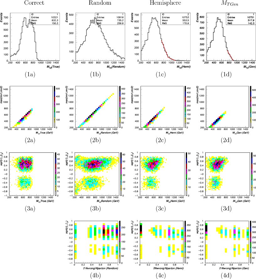
Figure 2: (1a)$-$(1d): $M_{T2}$ distributions.   (2a)$-$(2d): Distributions on a ($M_{T2}(m_{\tilde{\chi}_{1}^{0}})$, ${\rm sign}(-\beta^{2}_{12})\sqrt{|\beta^{2}_{12}|}$) plane.   (3a)$-$(3d): Distributions on a ($M_{T2}(m_{\tilde{\chi}_{1}^{0}})$, ${\rm sign}(-\beta^{2}_{12})\sqrt{|\beta^{2}_{12}|}$) plane.   (4b)$-$(4d): Distributions on a ($2N_{\rm wrong}/N_{\rm parton}$, ${\rm sign}(-\beta^{2}_{12})\sqrt{|\beta^{2}_{12}|}$) plane.   The correct, random, $M_{TGen}$ and hemisphere assignments are adopted in figures ($i$a), ($i$b), ($i$c) and ($i$d), respectively, where $i=1-4.$   We generate $6\times 10^{4}$ events at Point 5 with 7 TeV proton centre of mass energy.

Fig. 2 (1a) shows the $M_{T2}$(true) distribution in parton level. As can be seen, the $M_{T2}$(true) distribution has a sharp endpoint at $\max\{m_{\tilde{q}},m_{\tilde{g}}\}=m_{\tilde{q}}\simeq 910$ GeV. We generate 60000 events at Point 5 with 7 TeV proton centre of mass energy, and ISR is not included. We apply the following “minimal cuts” to reduce the standard model background

1.

$E_{T}^{\rm miss}>\max(100\,{\rm GeV},0.2M_{\rm eff}$),

2.

$M_{\rm eff}>500$ GeV,

3.

$N^{\rm jets(parton)}_{p_{T}>100\,{\rm GeV}}\geq 1$,

in addition, we also define

4.

$N^{\rm jets(parton)}_{p_{T}>50\,{\rm GeV}}\geq 4$  (“4 jet cut”),   or    $N^{\rm jets(parton)}_{p_{T}>200\,{\rm GeV}}\geq 2$  (“2 jet cut”),

for section 5.

If $v_{i}$ is not defined appropriately, $M_{T2}$ can exceed $\max\{m_{A_{1}},m_{A_{2}}\}$. Fig. 2 (1b) shows the $M_{T2}$ distribution where partons are randomly assigned into $v_{1}$ or $v_{2}$ so that each system has at least one constituents. We can see that the distribution has a large tail, and the endpoint structure is not seen.

To see what kinds of events and assignments generate large $M_{T2}$ values, we show distributions with the random assignment on ($M_{T2}$, $\max(m_{v1},m_{v2})$) and ($M_{T2}$, ${\rm sign}(-\beta^{2}_{12})\sqrt{|\beta^{2}_{12}|}$) planes in Fig. 2 (2b) and (3b), respectively. Here, $\beta^{2}_{12}\equiv\overrightarrow{\beta}_{1}\cdot\overrightarrow{\beta}_{2}$ is an inner product between velocity vectors of $A_{1}$ and $A_{2}$ in the lab frame. From figure (2b), we can see that the $M_{T2}$ is linearly dependent on the heavier of $m_{v1}$ and $m_{v2}$. Thus, the assignments that provide large $M_{T2}$ also provide large $m_{v_{i}}$. In addition, from figure (3b) we can see that the endpoint of the $M_{T2}$ distribution increases as increasing ${\rm sign}(-\beta^{2}_{12})\sqrt{|\beta^{2}_{12}|}$ from 0 to 0.8. The tail of the $M_{T2}$ distribution is mainly caused by the events with large ${\rm sign}(-\beta^{2}_{12})\sqrt{|\beta^{2}_{12}|}$. In such events, $A_{1}$ and $A_{2}$ are highly boosted into back-to-back.

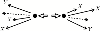
Figure 3: A schematic picture of an assignment that provides a dangerously large $M_{T2}$ value in an event with $\sqrt{\hat{s}}\gg M_{1}+M_{2}$. Dashed arrows represent the missing particles. Visible objects are grouped into $X$ or $Y$.

Fig. 3 is a schematic picture of a wrong assignment that provides large $M_{T2}$. In the picture two initial particles are highly boosted into back-to-back, and daughter particles are incorrectly assigned into groups, $X$ and $Y$. As can be seen, if two daughters, $i$ and $j$, have different origin, the back-to-back boost makes their angle $\theta_{ij}$ and momentum magnitudes large. This results a large invariant mass of the visible systems.

For the events with large back-to-back boosts and two daughter particle momenta from the same sparticle makes small angle compared to ones from different origin. The idea of hemisphere algorithm is based on this observation, although the angle $\theta_{ij}$ is modified into more elaborate distant measure, $d$. Interestingly, even if the algorithm fails to find the correct assignment, $m_{v_{i}}$ would not be too large because members in the same group have relatively small $d$. In the algorithm, the highest $p_{T}$ jet is assigned into a different group from the one contains the jet with the largest $p_{T_{i}}\Delta R(p(J_{1}),p(i))$. This also prevents from making $m_{v_{i}}$ too large.

Fig. 2 (1c), (2c) and (3c) correspond to (1b), (2b) and (3b), respectively but hemisphere algorithm is used. From figures ($i$c) ($i=1,2,3$), we can see that the tails in figures ($i$b) are removed significantly, and the endpoint structure at $\max\{m_{A_{1}},m_{A_{2}}\}$ is recovered. Fig. 2 (4b) and (4c) shows distributions on ($2N_{\rm wrong}/N_{\rm parton}$, ${\rm sign}(-\beta^{2}_{12})\sqrt{|\beta^{2}_{12}|}$) planes for the random and hemisphere algorithm, respectively. Here, $N_{\rm wrong}$ is the number of wrong assignments. As expected, in events with large ${\rm sign}(-\beta^{2}_{12})\sqrt{|\beta^{2}_{12}|}$ ($\hskip 3.00003pt\raisebox{1.72218pt}{$>$}\raisebox{-3.01385pt}{$\sim$}\hskip 3.00003pt0.4$), the algorithm successfully selects the correct assignment with high probabilities. Compared to (4b), the improvement is significant. Note that large back-to-back boosts require $\sqrt{\hat{s}}\gg m_{A_{1}}+m_{A_{2}}$, where $\sqrt{\hat{s}}$ is centre of mass energy of colliding partons. An event sample used in Fig. 2 is at Point 5 with $\sqrt{S}=7$ TeV, which has the largest sparticle mass scale and the smallest centre of mass energy of protons in our samples shown in Table. 1. The efficiencies of the algorithm would be better for the other samples, or at higher $\sqrt{S}$

Another known algorithm is $M_{TGen}$ method. By its construction, this variable is smaller than or equal to $M_{T2}$(true) in event by event basis. Fig 2 ($i$d) ($i=1-4$) correspond to ($i$c) but $M_{TGen}$ method is adopted. From figure (4d), we can see that $M_{TGen}$ can select the correct assignment in events with large ${\rm sign}(-\beta^{2}_{12})\sqrt{|\beta^{2}_{12}|}$ ($\hskip 3.00003pt\raisebox{1.72218pt}{$>$}\raisebox{-3.01385pt}{$\sim$}\hskip 3.00003pt0.4$) as hemisphere algorithm. This is because in such events all wrong assignments can provide larger $m_{v_{i}}$ than that from the correct assignment because of the back-to-back boost.

Compared to hemisphere algorithm, $M_{TGen}$ distribution does not have a tail beyond $\max\{m_{A_{1}},m_{A_{2}}\}$ in parton level without ISR. We fit distribution (1c) to two linear functions, $f(M_{T2})=a_{\pm}(M_{T2}-M_{T2}^{\rm edge})+b$ for ${\rm sign}(M_{T2}-M_{T2}^{\rm edge})=\pm 1$, and (1d) to a linear function, $f(M_{TGen})=c-dM_{TGen}$. The fitted endpoints is $912.2\pm 9.6\,$GeV for (1c). On the other hand, $M_{TGen}^{\rm edge}=c/d$ are $906.8\pm 85.2$ for (1d). The main source of the large error in the $M_{TGen}^{\rm edge}$ is poor statistics near the endpoint region. To improve the error we can fit the distribution away from the endpoint. However in this case, the central value become lower than the input squark mass. Both results are consistent with $\max\{m_{\tilde{q}},m_{\tilde{g}}\}=m_{\tilde{q}}\simeq 910$ GeV.

As can be seen, the slope of the $M_{TGen}$ distribution is sharper than that of the $M_{T2}$ distribution with hemisphere algorithm. This feature relies on the property that the $M_{TGen}$ can not exceed the mass of a sparticle. We will show that this property is not held for the $M_{TGen}$(min) and the $M_{TGen}^{\rm mod}$(min). In the rest of this paper, we adopt hemisphere algorithm unless it is explicitly stated, because both algorithms have similar performance but $M_{TGen}$ calculation is more computational intensive. In addition, as we will show later, hemisphere algorithm can be also applied to find out decay topology in the events.

4 Parton level $M_{T2}(\rm min)$ and $M_{T2}^{{\rm mod}}({\rm min})$ distributions with and without ISR

In section 2, we defined $M_{T2}$(min) and $M_{T2}^{\rm mod}({\rm min})$ variables for gluino mass measurement. The idea of these variables is that the events above the $M_{T2}$(true) endpoint can be removed by subtracting the hardest ISR jet. Although those variables are designed for the events with a hard ISR jet, we first show parton level $M_{T2}$(min) and $M_{T2}^{\rm mod}({\rm min})$ distributions without ISR. SUSY processes are the mixture of the events with and without hard ISR jets. We therefore check that parton level $M_{T2}$(min) and $M_{T2}^{\rm mod}({\rm min})$ distributions do not “collapse” near the endpoint by removing a parton from sparticle decays.

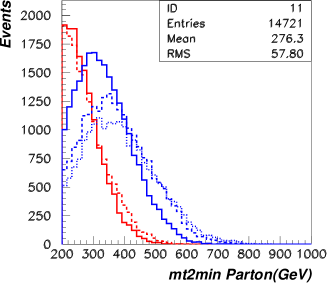
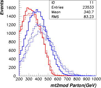
Figure 4: Left; $m_{T2}({\rm min})$ distributions in parton level. Right; $m_{T2}^{\rm mod}({\rm min})$ distributions in parton level. Red-solid, -dashed, Blue-solid, -dashed and -dotted distributions correspond to Points 1, 2, 3, 4 and 5, respectively. We generate 60000 events at 14 TeV.

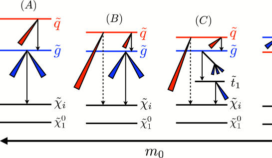
Figure 5: Schematic picture depicting decay patterns for various mass spectra. A, B, C and D correspond to $m_{\tilde{q}}\gg m_{\tilde{g}}$, $m_{\tilde{q}}>(m_{\tilde{t}_{1}}+m_{t})>m_{\tilde{g}}$, $m_{\tilde{q}}>m_{\tilde{g}}>(m_{\tilde{t}_{1}}+m_{t})$ and $m_{\tilde{g}}>m_{\tilde{q}}$, respectively. Red and blue triangles represent jets from squark and gluino decays, respectively. Dashed arrows represent the decays are not main modes.

Fig. 4 (left) shows $M_{T2}({\rm min})$ distributions, where red-solid and -dashed distributions correspond to Points 1 and 2 ($m_{\tilde{g}}>m_{\tilde{q}}$), and blue-solid, -dashed and -dotted ones correspond to Points 3, 4 and 5 ($m_{\tilde{q}}>m_{\tilde{g}}$), respectively. Here we generate 60000 events at 14 TeV, and the minimal cuts defined in the previous section is applied. For Points 3, 4 and 5, the endpoints of the distributions roughly agree with the gluino masses 636, 646 and 651 GeV, respectively. On the other hand, for Points 1 and 2, the endpoints of the distributions are about $100-200$ GeV smaller than the input gluino masses.

The difference in the distributions at Points 1, 2 and those at Points 3, 4, 5 comes from the ordering on the gluino masses. Fig. 5 shows various mass spectra and corresponding decay patterns. Points 5 and 3, 4 correspond to types $A$ and $B$ in Fig. 5, respectively. A squark dominantly decays to $j\tilde{g}$, and a gluino decays to $jj\tilde{\chi}_{i}$ in the region. Although there is a large mass hierarchy between gluino and weak gauginos, $p_{T}$ of jets from the gluino decay are relatively mild because of the three body decay. Consequently, the events tend to have multiple jets with modest $p_{T}$.

On the other hand, mass spectra at Points 1 and 2 correspond to type $D$ in Fig. 5. A squark decays to two body final state $j\tilde{\chi}_{i}$ producing a high $p_{T}$ jet for the mass spectrum. Because a gluino decays to $j\tilde{q}$, SUSY events usually contain two high $p_{T}$ jets from the squark decays. If we subtract one of the high $p_{T}$ jets from the event, the remaining system loose too much energy and calculated $M_{T2}$ can not reach at the gluino mass.

A variable $M_{T2}^{\rm mod}$(min) is designed to reconstruct the gluino mass in type $D$ spectrum. In the definition, we do not subtract the two highest $p_{T}$ jets. Fig. 4 (right) shows $M_{T2}^{\rm mod}({\rm min})$ distributions in parton level, where the colour and line schemes are the same as the LHS figure. The endpoints for Points 1 and 2 are consistent with the input gluino masses 612 and 629 GeV, respectively. On the other hand, for Points 3, 4 and 5, the endpoints are about 100 GeV larger than the gluino masses. The events above the input gluino mass are mostly $\tilde{g}$-$\tilde{q}$ production events. This suggests that $M_{T2}$(min) and $M_{T2}^{\rm mod}$(min) should be used for appropriate mass spectrum and decay pattern. Namely we need to know the mass ordering of gluino and squark in the gluino measurement. We will discuss this point in the next section.

$M_{TGen}^{\rm mod}$(min) and $M_{TGen}^{\rm mod}$(min) variables can be defined analogously to $M_{T2}^{\rm mod}$(min) and $M_{T2}^{\rm mod}$(min), respectively. The left figure in Fig. 6 shows comparisons between $M_{T2}$(min) (black) and $M_{TGen}$(min) (red) distributions at Point 5. Both the distributions have endpoints near the input gluino mass but also tails which mainly come from $\tilde{q}$-$\tilde{g}$ production events. Similarly, the right figure in Fig. 6 shows $M_{T2}^{\rm mod}$(min) (black) and $M_{TGen}^{\rm mod}$(min) (red) distributions at Point 1. The endpoints are given by the input squark mass. At Point 1 ($m_{\tilde{g}}>m_{\tilde{q}}$), $\tilde{g}$-$\tilde{g}$ production events can produce $M_{T2}^{\rm mod}$(min) and $M_{TGen}^{\rm mod}$(min) larger than the squark mass. However the cross section of this production process is subdominant and the tails are tiny. To reconstruct the gluino mass, inclusion of ISR is necessary as we will show in the next section. We may slightly improve the distributions by adopting $M_{TGen}^{(\rm mod)}$(min) instead of $M_{T2}^{(\rm mod)}$(min), although it would be computational intensive especially for the events with a large number of jets.

Figure 6: Left; parton level $m_{T2}({\rm min})$ (black) and $m_{TGen}({\rm min})$ (red) distributions at Point 5. Right; parton level $m_{T2}^{\rm mod}({\rm min})$ (black) and $m_{TGen}^{\rm mod}({\rm min})$ (red) distributions at Point 1.

We now discuss effect of hard initial state radiations associated with hard processes at LHC. It was explicitly shown in Ref.[26] that

1. The hardest ISR parton in $\tilde{g}$ and $\tilde{q}$ production processes could be harder than partons coming from $\tilde{g}$ three body decay $\tilde{g}\rightarrow jj\tilde{\chi}^{0}_{1}$. The ISR causes endpoint smearing of the inclusive $M_{T2}$ distributions. Significant events appears beyond the $M_{T2}$(true) endpoint for $\tilde{g}$-$\tilde{g}$ production when the $M_{T2}$ is calculated from the four highest $p_{T}$ jets.

2. The $M_{T2}({\rm min})$ distribution is less affected by ISR, because the leading ISR effect can be removed. It is explicitly shown that $M_{T2}^{\rm max}({\rm min})\simeq m_{\tilde{g}}$ for the process $pp\rightarrow\tilde{g}\tilde{g}$ when a gluino is forced to decay through three body decay mode $\tilde{g}\rightarrow jj\tilde{\chi}_{1}^{0}$.

	Point 1	Point 3	Point 5	Point 3’
$\sigma(\tilde{g}\tilde{g}j)$(inclusive) /$\sigma(\tilde{g}\tilde{g})$ (exclusive)	1.48	1.61	1.72	1.42
$\sigma(\tilde{g}\tilde{q}j)$(inclusive) /$\sigma(\tilde{g}\tilde{q})$(exclusive)	0.69	0.77	0.84	0.69

Table 3: Ratio between the number of events with and without a hard ISR parton. See text for the detail

The ratio of events with a hard ISR to those without any hard ISR is summarized in Table 3. Here we show the ratio of the number of events, $N$(inclusive $\tilde{g}\tilde{g}j$ or $\tilde{g}\tilde{q}j$ sample)/$N$(exclusive $\tilde{g}\tilde{g}$ or $\tilde{g}\tilde{q}$ sample) calculated by Madgraph/Madevent[55] with Pythia parton shower[56]. Here, the “exclusive sample” is generated from $\tilde{g}$-$\tilde{g}$ or $\tilde{g}$-$\tilde{q}$ process with parton shower, but if parton shower is resolved, namely if a cluster of the partons is isolated from the initial state with more than a certain $k_{T}$ distance, the event is rejected. On the other hand the “inclusive sample” means the events generated from $pp\rightarrow\tilde{g}\tilde{g}j$ or $\tilde{g}\tilde{q}j$ matrix elements with full parton showers, where $j$ denotes gluon or quark. Again, if the event does not have a resolved parton cluster, the event is rejected. Altogether, there is no overlap between exclusive and inclusive samples. The parton level distribution of the “matched sample” is therefore the sum of the events of the inclusive sample and exclusive sample. The $k_{T}$ cut off scale is chosen so that there are no discontinuity in the total distribution. As it has already discussed in Ref.[26], the fraction of the inclusive events in $\tilde{g}\tilde{g}j$ matched samples is always higher than that in $\tilde{g}\tilde{q}j$ matched samples. This is because the difference in colour factors between $\tilde{g}$ and $\tilde{q}$.

Figure 7: Left: the $p_{T}$ distribution of ISR for $\tilde{g}\tilde{g}j$ process at Point 5 (solid), the highest $p_{T}$ decay products at Point 5(thick dotted) and Point 3’ (thin dotted). Right: ratio of the $p_{T}$ of the third and first $p_{T}$ partons from gluino decays at Point 1 (solid) Point 5 (thick dashed) and Point 3’(thin dashed) for the same process. The distributions are scaled from 20000 $\tilde{g}\tilde{g}j$ matched events to 1000 events at each point.

In Fig. 7 (left) we show the $p_{T}$ distribution of the ISR parton at Point 5 (a solid line). The $p_{T}$ is 200 GeV in average. The $p_{T}$ distributions of the ISR are roughly the same for all model points in this paper. On the other hand, the $p_{T}$ distributions of the partons from squark/gluino decay are rather model parameter dependent.

In the same figure we show the $p_{T}$ distributions of the highest $p_{T}$ partons from $\tilde{g}$ decays for the $\tilde{g}\tilde{g}j$ matched sample at Point 5 (thick dotted) and at Point 3’ (thin dashed). The gluino dominantly decays through three body final state $\tilde{g}\to jj\tilde{\chi}_{i}$ at Point 5. At Point 3’ the mass spectrum corresponds to type $C$ in Fig. 5, where $m_{\tilde{g}}>(m_{\tilde{t}_{1}}+m_{t})$. In this type of spectrum, a gluino dominantly decays into two-body final state $\tilde{g}\to\tilde{t}_{1}t$, and the top and stop further decay to lighter particles. Thus, the highest $p_{T}$ jet is relatively soft compared to that of Point 5 and the scale of $p_{T}$ is close to that of ISR. On the other hand, the distribution of the highest $p_{T}$ jet at Point 1 is similar to that at Point 5.

Not only the distribution of the highest $p_{T}$ jet, but also the distribution of the other jets could be different. In Fig. 7 (right), we plot the distributions of $p_{T3}/p_{T1}$ at Points 1 (solid), 5 (thick dashed) and 3’ (thin dashed). At Point 1, the highest $p_{T}$ jet takes significant part of the total energy of the event because $\tilde{q}\rightarrow q\tilde{\chi}_{i}$ modes dominate. While at Point 5, four partons from the gluino three body decays have roughly the same order of $p_{T}$. At Point 3’, the tendency is even stronger.

Figure 8: The $p_{T}$ order of the ISR parton among all partons of the inclusive $\tilde{g}\tilde{g}j$ sample. Left, center and right figures are at Points 1, 5 and 3’ respectively.

In Fig. 8, we plot the distribution of $i_{\rm ISR}$ where $i_{\rm ISR}$ is the order of an ISR parton among all the $p_{T}$ ordered partons in the $\tilde{g}\tilde{g}j$ inclusive sample at Points 1 (left), 5 (middle) and 3’ (right). Distributions for $\tilde{q}\tilde{g}j$ inclusive sample are similar to those for $\tilde{g}\tilde{g}j$.

At Point 1, the average number of jets in the events are rather small, but about a half of the events has more than four partons with $p_{T}>50$ GeV for $\tilde{g}$-$\tilde{g}$ production. The probablity that the ISR parton becomes the 1st or the 2nd hardest parton is smaller than the one to be the 3rd hardest parton, because at this point a squark dominantly decays into $\tilde{\chi}_{i}$ and a high $p_{T}$ quark. At Point 5, a gluino decays into three body final state $jj\tilde{\chi}$. The ISR parton is one among the five highest $p_{T}$ partons in that case. Finally, at Point 3’, the ISR tends to be the highest $p_{T}$ jet. This is because, a gluino dominantly decays into $t\tilde{t}$ at this point. The average number of jets is large, and at the same time each of the jets from squark/gluino decay has relatively small $p_{T}$.

We now consider the events that contribute to the endpoint of the $M_{T2}({\rm min})$. For exclusive samples, the $M_{T2}({\rm min})$ endpoints should be smaller than those of the $M_{T2}$. Especially at Point 1, removing one of the two highest $p_{T}$ partons from the system reduce the events near the endpoint too much as discussed previously. Instead of using the $M_{T2}({\rm min})$, we use $M_{T2}^{\rm mod}({\rm min})$ to obtain the endpoint. For the inclusive sample at Point 1, ISR tends to be the 3rd hardest parton of the event, and using the $M_{T2}^{\rm mod}({\rm min})$ is justified also from this point of view. In Fig. 9 we show the parton level distributions of $M_{T2}^{\rm mod}({\rm min})$ and $M_{T2}({\rm min})$ for the $\tilde{g}\tilde{g}j$ matched samples. The number of events near the input gluino mass 612 GeV is quite small for the $M_{T2}({\rm min})$, while significant events remain for the $M_{T2}^{\rm mod}({\rm min})$ in the same region. Using the $M_{T2}^{\rm mod}({\rm min})$ distribution clearly improves the sensitivity to the gluino mass.

Figure 9: Parton level $M_{T2}({\rm min})$(a solid line) and $M_{T2}^{\rm mod}({\rm min})$(a dashed line) distributions for the matched $\tilde{g}\tilde{g}j$ at Point 1. The $M_{T2}^{\rm mod}({\rm min})$ distribution has more events near the endpoint because of the events that ISR jets are correctly removed by the minimization. The distributions are based on 40000 matched $\tilde{g}$-$\tilde{g}$ events generated by Madgraph.

Figure 10: Parton level $M_{T2}$(min) distributions of (top left) matched $\tilde{g}\tilde{g}j$ sample and (bottom left) matched $\tilde{q}\tilde{g}j$ sample calculated by Madgraph + Pythia. The corresponding jet level distributions obtained by HERWIG with detector simulation are placed in the right; (top right) $\tilde{g}$-$\tilde{g}$ production and (bottom right) $\tilde{q}$-$\tilde{g}$ production.

For Point 5, the minimization of $M_{T2}(i)$ over the five hardest jets is reasonable in removing the ISR jet, because the $i_{\rm ISR}$ distribution shown in Fig. 8 is flat for the five hardest jets. The endpoint of the $M_{T2}({\rm min})$ distribution for inclusive $\tilde{g}\tilde{g}j$ production would be near the input gluino mass because significant events has a hard ISR jet. The $M_{T2}({\rm min})$ endpoint of the $\tilde{q}$-$\tilde{g}$ exclusive sample would also be near the gluino mass. This is because if we remove the parton from $\tilde{g}\rightarrow\tilde{q}j$ decay, the system becomes $\tilde{g}$-$\tilde{g}$, and the endpoint for such events is given as the input gluino mass. Therefore, by minimizing over the five hardest jets, a relation $M_{T2}^{\rm mod,max}({\rm min})\simeq m_{\tilde{g}}$ is satisfied. The sum of the $\tilde{g}\tilde{g}j$ and no-ISR $\tilde{q}\tilde{g}$ productions provide the endpoint at $m_{\tilde{g}}$. Additional ISR jets for $\tilde{g}$-$\tilde{q}$ productions could lead the distribution that ends near the squark mass, which may smear the endpoint at $m_{\tilde{g}}$. Fortunately, the fraction of $\tilde{g}\tilde{q}j$ exclusive sample is less than a half of the total events at Point 5.

Of course, the shape of the distributions near the endpoints can only be estimated by Monte Carlo simulation. In Fig. 10, we show the parton level $M_{T2}({\rm min})$ distributions of the matched sample (left) at Point 5 generated by Madgraph/Madevent with Pythia, and compare it jet level distributions generated by HERWIG with detector simulation. Here the jet level event is reconstructed by the AcerDET[57] with jet energy smearing of $\delta E/E=50\,\%/\sqrt{(}E(GeV))$. Jet reconstruction of the AcerDET is replaced to the Cambridge-Aachen algorithm with $\Delta R=0.4$ using Fastjet[58].

The top figures are the $M_{T2}$(min) distributions for $\tilde{g}\tilde{g}j$ production sample and the bottom figures are for $\tilde{g}\tilde{q}$ production. At Point 5, the parton level endpoint for the $\tilde{g}$-$\tilde{q}$ sample is around 700 GeV, which is consistent with the input gluino mass, 651 GeV and far below the input squark mass, 910 GeV. Note that the left and right distributions are roughly consistent although 1) Our Madgraph samples include matrix element contribution of the hardest ISR parton, 2) Our jet level samples obtained by HERWIG include all ISR effects in parton shower approximation. 3) HERWIG takes care spin correlation of matrix elements and all decay processes, while Pythia does not for sparticle decays.

5 The results of jet level simulations

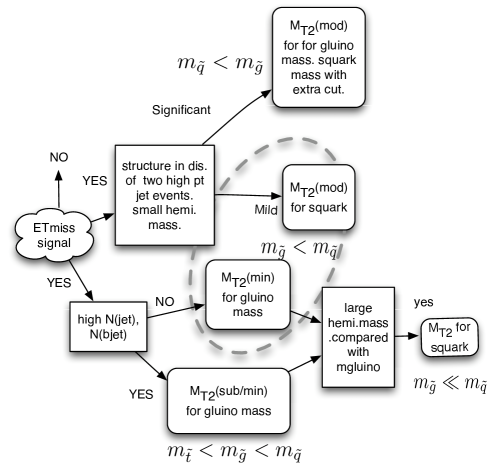
Figure 11: Flowchart of the ISR improved $M_{T2}$ analysis

In this section, we show jet level results and discuss mass parameter determination by $M_{T2}$(min) and $M_{T2}^{\rm mod}$(min). To make our discussion clear, we show the steps for mass determination in Fig. 11. We will see the importance of the proper choice of improved $M_{T2}$ depending on the observed event distribution.

5.1 $M_{T2}$ distributions and effect of the ISR

Figure 12: $M_{T2}$ distributions at Points 1, 3 and 5 in parton level (left) and in jet level (right). We generate 60000 SUSY events at 14 TeV.

We compare the parton level $M_{T2}$ distributions with out ISR (left) to jet level ones (right) in Fig. 12. We generate the evens by HERWIG+AcerDET+Fastjet as discussed in previous secton. In the left figure, the distribution reduces rather quickly toward $M_{\rm max}\equiv\max(m_{\tilde{g}},m_{\tilde{q}})$ and there are tails beyond $M_{\rm max}$ due to mis-reconstruction of hemispheres. On the other hand, the jet level distributions at Points 1 and 3 do not show structures at neither the squark nor gluino masses. Especially, the number of events beyond 750 GeV at Point 5 is not much different from that of Point 3 in jet level.

In the previous studies[24], the endpoint of $M_{T2}$ distributions are consistent with $M_{\rm max}$. The difference comes from the choice of the squark and gluino mass scale. In the paper, the gluino mass is around 800 GeV and the squark masses are taken from 881 GeV to 1561 GeV. As the squark and gluino masses increase, relative importance of the ISR jet reduces as the average $p_{T}$ of the sparticle decay products increases linearly with the sparticle mass, while average $p_{T}$ of the ISR jet does not increase so quickly. We take the scale of SUSY parameters rather light ($m_{\tilde{g}}\hskip 3.00003pt\raisebox{1.72218pt}{$<$}\raisebox{-3.01385pt}{$\sim$}\hskip 3.00003pt700$ GeV) in this paper so that squark and gluino masses are in the discovery region at the early stage of the LHC.

The ISR effect reduces significantly when $m_{\tilde{q}}$ is increased for fixed $m_{\tilde{g}}$. At Point 5, where the sum $m_{\tilde{q}}+m_{\tilde{g}}$ is 350 GeV higher than that at Point 1, the endpoint is roughly at the input value, 910 GeV. The reduction of the ISR effect may be understood as follows. At this point, there are large mass difference between squark and gluino and the endpoint is saturated by $M_{T}$ of the squark hemisphere, when hemisphere reconstruction is correct. The ISR jet has to be grouped into the “squark hemisphere” rather than the “gluino hemisphere” for the evnets contaminating beyond the endpoint, unless the $p_{T}$ of the jet is very high.

We compare the parton level distribution and the jet level distribution at Point 5 ($m_{\tilde{u}_{L}}=913$ GeV) more quantitatively in Fig. 13 (left). We found a linearly decreasing region of the $M_{T2}$ distribution is close to that of the parton level one. Fitting it by a linear function $f(M_{T2})=a+bM_{T2}$ for both signal and tail regions, we find “kink” position at 887 GeV for jet level and 882 GeV for parton level with errors around 10 % and 6 % respectively, which roughly agree with the squark mass.

In Fig. 13 (right), we also show the distributions at Point 4 ($m_{\tilde{u}_{L}}=837$ GeV). The endpoint is more difficult to see, although slopes of the two distributions agree between 650 $-$ 800 GeV. Extracting the mass scale from the distribution requires the detailed comparison between Monte Carlo and data, and it is not the scope of this paper. Therefore we move on to the $M_{T2}({\rm min})$ distributions which remove the hardest ISR jet efficiently.

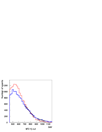
Figure 13: Comparison between parton level $M_{T2}$ (solid lines) and jet level $M_{T2}$ (dashed lines) distributions at Points 5 (left) and 4 (right). We generate 60000 events and apply the 4 jet cut. In the left figure fitting lines are also shown.

5.2 Events with Two high $p_{T}$ jets and proper choice of ISR improved $M_{T2}$ for gluino mass determination

In CMSSM like parameter region, event topologies are significantly different between the cases of $m_{\tilde{g}}>m_{\tilde{q}}$ (Points 1, 2, 1’ and 2’) and $m_{\tilde{q}}>m_{\tilde{g}}$ (Points 3, 4, 5, 3’, 4’ and 5’). As we discussed in section 4, in $m_{\tilde{q}}>m_{\tilde{g}}$ region, squarks mainly decay to $j\tilde{g}$, and the $j\chi_{i}$ mode is subdominant. On the other hand, in $m_{\tilde{g}}>m_{\tilde{q}}$ region, $\tilde{q}\to j\chi_{i}$ is the main mode and events contain two high $p_{T}$ jets. It is likely that the two hard jets are selected as the seeds of hemisphere reconstruction and thus assigned into different groups. Because each group has only one hard object, the masses of both visible systems are expected to be small. On the other hand, in $m_{\tilde{q}}>m_{\tilde{g}}$ region, each visible system may have two modest jets from gluino three body decays, and the mass scale of visible systems represent the gluino mass.

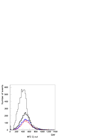
Figure 14: The jet level $M_{T2}$ distributions at Points 1 (black dotted), 3 (black solid), 4 (blue oslid) and 5 (red dashed) for the events with at least two jets with $p_{T}>200$ GeV. The sharp edge at Point 1 is mostly consisted by the events with $n_{50}\leq$4. The distribution at Point 2 is similar to that at Point 1 and is not shown.

As discussed in the previous sections, the number of events beyond $\min(m_{\tilde{g}},m_{\tilde{q}})$ will be significantly reduced for $M_{T2}({\rm min})$ distribution. However, the shape of the distribution depends on the mass spectrum, and decay pattern. Especially the $M_{T2}({\rm min})$ distribution would be flat near the expected endpoint at Point1 1 and 1’, and we should use $M_{T2}^{\rm mod}({\rm min})$ distribution to obtain the gluino mass. Another way to say, to obtain the correct gluino mass, we need criteria to use $M_{T2}^{\rm mod}({\rm min})$ instead of $M_{T2}({\rm min})$ from experimental data.

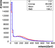
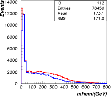
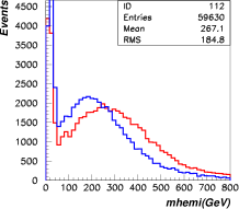
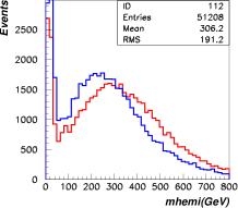
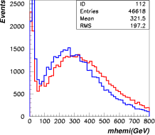
Figure 15: Jet level $m_{v}$ distributions for the hemisphere reconstruction. The $m_{v}^{(1)}$ and $m_{v}^{(2)}$ are superposed. Red (Blue) distributions in figures (1) $-$ (5) correspond to Points 1 $-$ 5 (1’ $-$ 5’), respectively.

The fraction of events which survive under the 2 jet cut is the one of the key observation to make the choice. In Fig. 14, we show the distribution of the events with at least two jets with $p_{T}>200$ GeV. The number of events after the cut is large at Point 1 (a black dotted line), compared to those at Points 3 $-$ 5. As discussed already, this is because the $\tilde{q}\to j\tilde{\chi}_{i}$ mode dominates at Point 1. If we see the excess, we should use $M_{T2}^{\rm mod}({\rm min})$. Structure in $M_{T2}$ distribution under the 2 jet cut might also be useful for determination of ordering of squark and gluino masses. We observe a sharp endpoint at the true squark mass (600 GeV) at Point 1. Although the number of the events after the 2 jet cuts is rather small, such structure also exists at Point 3. This is due to the squark decay into electroweak inos with significant branching ratio at this point. We will discuss about mixed use of $M_{T2}^{\rm mod}({\rm min})$ and $M_{T2}({\rm min})$ at Points 3 and 3’ in the next subsection.

Alternatively, one can use hemisphere mass $m_{v}$ to estimate fraction of the events that have gone though $\tilde{q}\rightarrow j\chi$ decays. Red (Blue) distributions in Fig. 15 (1) $-$ (5) show the jet level $m_{v}$ distributions for Points 1 $-$ 5 (1’ $-$ 5’), respectively. Here $m_{v}^{(1)}$ and $m_{v}^{(2)}$ are superposed in the distributions. The shape of the distributions are very different between $m_{\tilde{g}}>m_{\tilde{q}}$ and $m_{\tilde{q}}>m_{\tilde{g}}$ cases. In $m_{\tilde{g}}>m_{\tilde{q}}$ region (See Figs. 15 (1) and (2).), the distributions have a sharp peak at $m_{v}=0$, and the fraction of the other events are small. On the other hand, in $m_{\tilde{q}}>m_{\tilde{g}}$ (See Figs. 15 (3), (4) and (5).), the distributions have another peak around $m_{\tilde{g}}/2$, which is the contributions from $\tilde{g}\to\tilde{\chi}jj$ mode. The fraction of the events with $m_{v}\sim 0$ becomes small. This suggests that the shape can give us information of the ordering of gluino and squark masses. We can also study the hemisphere mass after removing the jet $i_{\rm min}$, $m_{v}^{(1)}(i_{\rm min})$ and $m_{v}^{(2)}(i_{\rm min})$, where $M_{T2}({\rm min})=M_{T2}(i_{\rm min})$. The fractions of the events with $\min(m_{v}^{(1)}(i_{min}),m_{v}^{(2)}(i_{min}))<50$ GeV are 73 %, 45 % and 35 % at Points 1, 3 and 5, respectively.

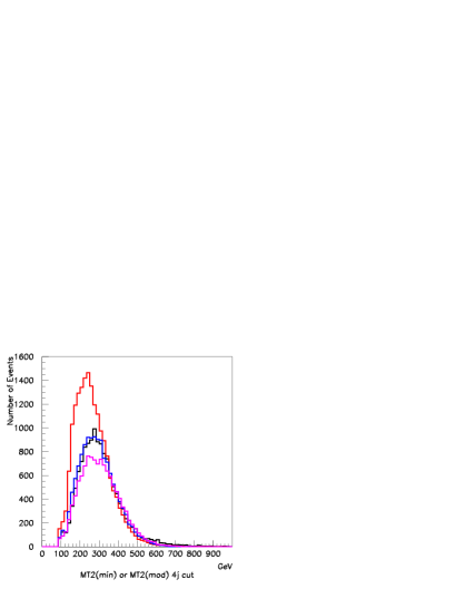
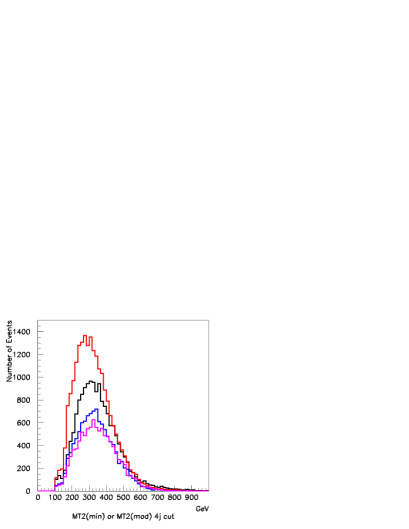
Figure 16: Left) $M_{T2}^{\rm mod}({\rm min})$ (Point 1’:black) and $M_{T2}({\rm min})$ distributions (Points 3’:red, 4’:blue, 5’:purple). Right ) $M_{T2}^{\rm mod}({\rm min})$ (Point 1: black ) and $M_{T2}({\rm min})$ distributions (Points 3:red, 4:blue, 5:purple). The mass of gluinos are from 522 $-$ 558 GeV at Points 1’ $-$ 5’ and 612 $-$ 651 GeV at Points 1 $-$ 5, respectively.

point	$a$	$\delta a$	$b$	$\delta b$	$a/b$	gluino mass
1	2045	84	3.42	0.16	598	612
2	2103	107	3.38	0.20	623	620
3	2285	64	3.86	0.13	592	635
4	1288	57	2.10	0.10	612	646
5	1178	82	1.90	0.13	620	651
1’	1592	70	2.98	0.16	534	522
2’	1571	68	2.95	0.15	533	528
3’	1842	67	3.66	0.15	502	541
4’	1765	69	3.37	0.15	524	550
5’	1514	81	2.77	0.17	547	558

Table 4: The results of linear fits of the distributions in Fig. 16 near the endpoint. The fitting function is a simple linear function $f=a-bM_{T2}$. For Points 1, 2, 1’ and 2’, $M_{T2}^{\rm mod}({\rm min})$ distributions are used, and $M_{T2}({\rm min})$ for the others.

Based on the discussions above, we decide to use $M_{T2}^{\rm mod}({\rm min})$ for Points 1’, 2’, 1 and 2, and $M_{T2}({\rm min})$ for 3’ $-$ 5’ and 3 $-$ 5 to determine the gluino masses. The jet level distributions are shown in Fig. 16. The left figure shows the distributions at Points 1’ $-$ 5’ and the right figure show the distributions at Points 1 $-$ 5’. The fomar have endpoints around 500 GeV while the latter is around 600 GeV.

As we have seen in the parton level distribution, it is not good idea to focus on the events too close to the endpoint when we use the hemisphere algorithm to define $M_{T2}$. Unlike $M_{TGen}$, the algorithm tend to preserve the number of events near the endpoint, but there is a tail beyond the true endpoints because of the hemisphere misreconstruction. Therefore we fit the distributions to linear functions from the bin with the hight half of the maximum to the bin at the 1/10 $\sim$ 1/6 of the maximum. The results of the fitting functions, $f=a-bM_{T2}^{({\rm mod})}({\rm min})$, are listed in Table 4. The errors are typically 7 % and section of the line $b/a$ are consistent with the corresponding gluino masses. The fitting function adopted here is too simple, leading $\chi^{2}/n_{\rm d.o.f}$ are around 2.

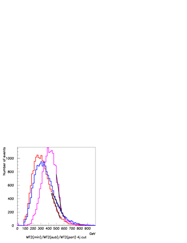
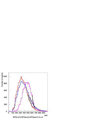
Figure 17: $M_{T2}({\rm min})$ distributions (red lines), $M_{T2}({\rm sub})$ distributions (blue line) and parton level $M_{T2}$ distributions for $\tilde{g}$-$\tilde{g}$ production (purple lines). The left and right figures correspond to Points 5’ and 5, respectively. Fitting curves are also shown in the figures.

In the previous paper, we have proposed $M_{T2}({\rm sub})$ to determine the gluino mass when $m_{\tilde{g}}<m_{\tilde{q}}$. The endpoint of $M_{T2}({\rm min})$ distribution agrees with the gluino mass better then $M_{T2}({\rm sub})$. The minimization among the possible assignment of jets from $\tilde{q}\rightarrow\tilde{g}q$ decay among high $p_{T}$ jets ensures $M_{T2}({\rm min})$ distribution in $\tilde{q}\tilde{g}$ production is below $m_{\tilde{g}}$ when there are no significant ISR jet. We show $M_{T2}$(min) (red lines) and $M_{T2}$(sub) (blue lines) the distributions at Points 5’ (left) and 5 (right) in Fig. 17 with fitting curves near the endpoint. For comparison, parton level $M_{T2}$ distributions for $\tilde{g}$-$\tilde{g}$ samples without ISR jets are also shown by purple lines. The $M_{T2}({\rm sub})$ distributions suffer higher tails and tend to overshoot the true endpoints. Exceptional case is Point 3’, which we will discuss separately.

5.3 Squark mass determination

In this section we discuss squark mass determination from the experimental data. In Fig. 18, we show the distributions of $M_{T2}^{\rm mod}({\rm min})$ at Points 1’ (left) and 1 (right) after 2 jet cut. Under the cut, the $\tilde{q}$-$\tilde{q}$ production events are significant part of the survived events, because events with $\tilde{g}\to\tilde{t}t$ tend to be rejected. The structure due to the $\tilde{q}$-$\tilde{q}$ production events can be seen in the total distribution. The endpoints of $\tilde{q}$-$\tilde{q}$ parton level distributions (the thick dotted lines) are consistent with the positions of the edge structure in the jet level distributions (the solid lines), on the other hand $\tilde{g}$-$\tilde{g}$ distribution (the thin dashed lines) are negligible. Taking $M_{T2}^{\rm mod}({\rm min})$ reduces the contamination of $\tilde{q}$-$\tilde{g}$ production beyond the edge.

The jet distribution reduces very quickly near the endpoint. At Point 1’, we fit the distribution by two linear functions. At point 1 we fit the distribution to a quadratic function bellow the kink and a linear function beyond the kink. The obtained kink position is at 483 (540.0) GeV at Point 1’ (1). The values are very close to the input squark masses, and much smaller than gluino masses. Errors in the values are around 7 %.

Figure 18: $M_{T2}^{\rm mod}({\rm min})$ distributions after the two jet cut (solid lines), and parton level $M_{T2}$ distributions of $\tilde{q}\tilde{q}$ (thick dashed lines ) and $\tilde{g}\tilde{g}$ distributions (thin dashed lines). The left and right figures are for Points 1’ and 1, respectively.

Now we show distributions at Points 3’ and 3. The squark masses is around 619 (734) GeV at Point 3’ (3). At these model points, the squarks are heavier than the gluino but the decay $\tilde{q}\rightarrow j\chi_{i}$ still has a significant branching ratio (See Table. 1). Especially the fraction of the events survives under 2 jets cut at Point 3 is larger than those at Points 4 and 5. Then there is a possibility to obtain the squark mass scale by fitting the $M_{T2}^{\rm mod}({\rm min})$ endpoint instead of $M_{T2}({\rm min})$. In Fig. 19 we fit the events near the endpoint to a linear function. The endpoints of $M_{T2}^{\rm mod}({\rm min})$ distributions are 557.4 GeV and 676.1 GeV with about 6 % of statistical errors at Points 3’ and 3, respectively, higher than fitted endpoint of $M_{T2}({\rm min})$($\sim m_{\tilde{g}}$) listed in Table 4. Fits of the parton level $M_{T2}$ distirubtions of $\tilde{g}\tilde{q}$ production process lead 601 GeV and 706 GeV at Points 3’ and 3, respectively.

Point 3’ is a model point with special feature. At the point, gluino decays into $\tilde{t}t$ dominantly. It is easy to see that $\tilde{g}\rightarrow\tilde{t}t$ is the dominant gluino decay mode through the numbers of both jets and $b$-jets in the events. The parton level $M_{T2}$ distributions at Point 3’ is suppressed near squark and gluino masses. This is due to the softness of average jet $p_{T}$. We only use the jets with $p_{T}>50$ GeV. On the other hand, the average $p_{T}$ of the jets are small so that some jets from gluino decays are not taken into account in the mass reconstruction. We may reduce the $p_{T}$ cuts but in that case the probability to assign jets into the wrong hemisphere becomes so large and the endpoints are smeared. Indeed, the endpoint of the parton and jet level distribution is systematically lower than the input squark mass.

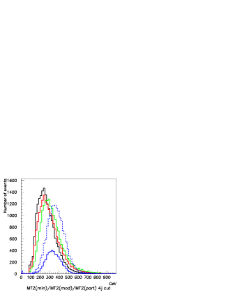
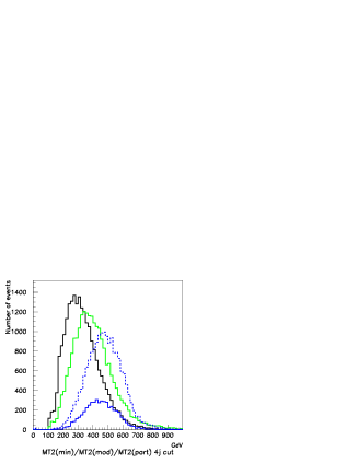
Figure 19: $M_{T2}({\rm min})$ (black) and $M_{T2}^{\rm mod}({\rm min})$ (green) distributions at Point 3’ (left) and Point 3 (right). The blue sold and blue dotted lines correspond to parton level $\tilde{g}\tilde{g}$ and $\tilde{g}\tilde{q}$ distributions, respectively. At Point 3 gluino decay into three body final state, while a gluino decays into a stop and a top at Point 3’. We also show a distribution of $M_{T2}({\rm sub})$ (red line) at Point 3’ whose endpoint is slightly lower than that of $M_{T2}^{\rm mod}({\rm min})$.

In the previous section, we have seen that the highest $p_{T}$ jet is likely to be the ISR at Point 3’ for $\tilde{g}$-$\tilde{g}$ production. The main decay modes of squarks are $\tilde{q}\to j\tilde{g}$, and $\tilde{q}\to j\tilde{\chi}_{i}$ mode is subdominant. Therefore removing the highest $p_{T}$ jet might be equally useful to remove the hard ISR in $\tilde{q}\tilde{g}j$ production. To check this, we also plot $M_{T2}$(sub) distribution in the same plot (red line). Both $M_{T2}$(sub) and $M_{T2}^{\rm mod}({\rm min})$ have similar endpoints.

6 Expectation at $\sqrt{s}=7$ TeV and $\int{\cal L}dt=1{\rm fb}^{-1}$

Currently the LHC is operated at 7 TeV and will accumulate $\int{\cal L}dt\simeq 1\,{\rm fb^{-1}}$. Although the aim of this paper is to improve SUSY parameter determination in general hadron collider by using ISR improved inclusive $M_{T2}$, the event distribution at 7 TeV and $1\,{\rm fb^{-1}}$ of luminosity is also our interest.

Again, we start with discussion of the $M_{T2}$ distribution at 7 TeV. Fig. 20 shows the $M_{T2}$ distributions at Points 3’ (red filled) and 5’ (blue filled). The figures are based on 30000 events, but the expected number of events by the end of 7 TeV run is smaller (See Table 1.).

The smearing due to ISR is smaller than those at 14 TeV shown by the open histogram by black solid lines. The distributions beyond the true masses (shown by $*$ marks and the lines) at 7 TeV are less than corresponding distributions at 14 TeV. Especially some structure remains around 600 GeV at Point 3’. At Point 5’, $M_{T2}$ distribution is straight between 600 GeV to 800 GeV, and the endpoint obtained by fitting it to a linear function roughly consistent with the squark mass. The $M_{T2}$ distribution is correlated with squark mass and may be used for mass determination by fitting the distribution to the template based on Monte Carlo simulation data.

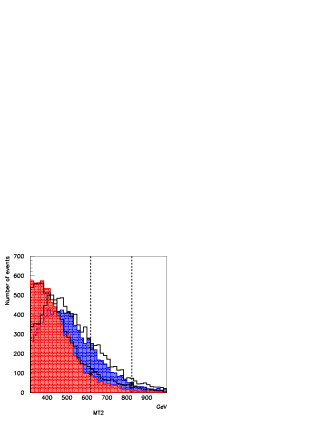
Figure 20: $M_{T2}$ distributions under the 4 jet cut at Points 3’ (red filled) and 5’(blue filled) and $\sqrt{s}=7$ TeV and those at 14 TeV( black solid line) . We use 30000 events at each model point.

In Fig. 21, we show the $M_{T2}^{\rm mod}({\rm min})$ distributions (bars) at Point 1’ (Type $D$ in Fig. 5.) with our 2 jet (left) and 4 jet (right) cuts together with the $M_{T2}$ distribution (green) under the same cut. In the figure we generate events corresponding to $\int{\cal L}=1\,{\rm fb^{-1}}$ at 7 TeV. The coincidence of the endpoint with the input squark/gluino masses (478/522 GeV) are already visible.

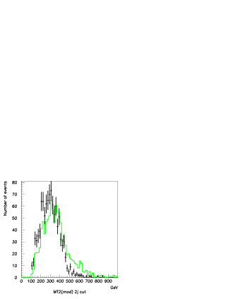
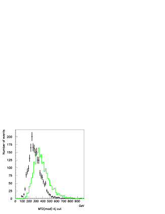
Figure 21: $M_{T2}$ distributions at 7 TeV and 1 fb^-1. $M_{T2}^{\rm mod}({\rm min})$ distirubtions with error bars at Point 1’ for the 2 jet cuts (left), and the 4 jet cut (right). Green lines show $M_{T2}$ distribution under the same cut.

Fig. 22 shows the $M_{T2}({\rm min})$ and $M_{T2}^{\rm mod}({\rm min})$ distributions at Point 3’, 3 and 5’ which have mass spectraType $A-C$. At Points 3 and 5’ production cross sections at 7 TeV are only around 1.7 pb and 2.5 pb and the distributions are under significant statistical flactuation. The $M_{T2}$ distribution ends around 800 GeV at Point 5, which reflects the input squark mass. Note that we have reason not to use $M_{T2}^{\rm mod}({\rm min})$ distribution for mass determination, because the number of the events which survives after 2 jet cut is smal. Therefore we do not show the $M_{T2}^{\rm mod}({\rm min})$ distribution in the figure.

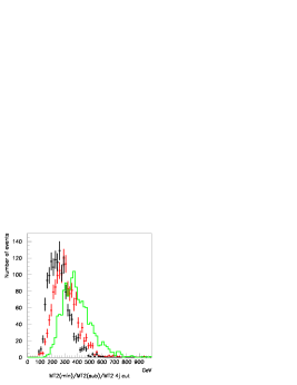
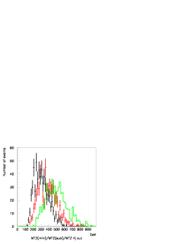
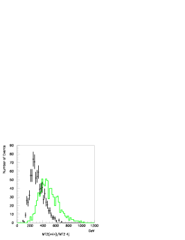
Figure 22: $M_{T2}$ distributions at 7 TeV and 1 fb^-1. The distributions of $M_{T2}({\rm min})$ (black bars) $M_{T2}^{\rm mod}({\rm min})$ (red bars) and $M_{T2}$ (green lines) for Point 3’ (left figure), 3 (central figure) and 5’ (right figure).

7 Conclusion

At the early stage of the LHC experiment, useful discovery channels are jets + $E_{\rm Tmiss}$ channel and jets+ 1 lepton + $E_{\rm Tmiss}$ . The luminosity is rather low, so we want to measure sparticle nature from inclusive measurement rather than exclusive and clean modes. While $M_{T2}$ is useful kinematical variables in measuring parent SUSY partilce masses, an inclusive definition proposed in[23] is not protected from smearing due to ISR.

In this paper we have proposed ISR improved inclusive $M_{T2}$ variables which might be useful to determine the squark and gluino masses separately. The modified $M_{T2}$ variables discussed in this paper are $M_{T2}({\rm min})$ and $M_{T2}^{\rm mod}({\rm min})$. Endpoints of those distributions represent squark and gluino masses as summarized in Table 5. Steps to identify sparticle masses are shown in Fig. 11. The $M_{T2}^{\rm mod}({\rm min})$ distribution is used for determination of gluino and squark masses for $m_{\tilde{g}}>m_{\tilde{q}}$ case as the algorithm keeps the highest $p_{T}$ jets in the hemisphere which is likely comes from squark two body decays for $m_{\tilde{q}}\gg m_{\chi}$ case. Even if $m_{\tilde{g}}\hskip 3.00003pt\raisebox{1.72218pt}{$<$}\raisebox{-3.01385pt}{$\sim$}\hskip 3.00003ptm_{\tilde{q}}$, $Br(\tilde{q}\rightarrow\chi q^{\prime})$ is large enough so that $M_{T2}^{\rm mod}({\rm min})$ is useful to determine $m_{\tilde{q}}$. On the other hand, $M_{T2}({\rm min})$ is important to determine $m_{\tilde{g}}$ when $m_{\tilde{g}}<m_{\tilde{q}}$ and the decay of $\tilde{g}$ is three body so that there are no dominant jets in the cascade decay.

Errors in mass determination which we have obtained from the endpoint fits are typically 6 $-$ 10 % for 60000 generated SUSY events. On the other hand, we expect 4000 (1000) events at 7 TeV and $\int{\cal L}dt=1\,{\rm fb^{-1}}$ and 380000 (10000) events at 14 TeV and $\int{\cal L}dt=10\,{\rm fb^{-1}}$ at Point 1 (5). Therefore, the model points with different gluino mass in Table 1 can be clearly separated using the $M_{T2}({\rm min})$ or $M_{T2}^{\rm mod}({\rm min})$ endpoints. We may identify an unique point in the squark and gluino mass parameter space up to the LSP mass uncertainty. This is very important meaning, because squark and gluino production crosss section is controlled by the masses up to small chargino and neutralino exchange contributions. We can cross check the predicted cross section to the observed number of events. In addition, the expected cross section would be significantly different if we change spin of the produced particles from scalar to fermion as is expected in Little Higgs models with T partity for example. Determination of the mass and decay pattern allows us to exclude/prove such models as well.

	2-jets $M_{T2}$	N(peak) of $M_{\rm hemi}$	N(b-jets)	determine S	determine G
$G>S$	significant clear edge	1	few	$M_{T2}^{\rm mod}({\rm min})$ 2-jets cut	$M_{T2}^{\rm mod}({\rm min})$ 4-jets cut
$S>G$ ($\tilde{g}\rightarrow\tilde{t}t$)	mild edge	2	many	$M_{T2}^{\rm mod}({\rm min})$ 2-jets cut or $M_{T2}({\rm sub})$	$M_{T2}({\rm min})$ 4-jets cut
$S>G$ ( $\tilde{g}\rightarrow jj\chi$)	mild edge	2	few	$M_{T2}^{\rm mod}({\rm min})$ 4-jets cut	$M_{T2}({\rm min})$
$S\ll G$	no clear edge	2	few	$M_{T2}$	$M_{T2}({\rm min})$ $M_{T2}({\rm sub})$

Table 5: Summary of the results obtained in this paper. G(S) denotes $m_{\tilde{g}}$ and $m_{\tilde{q}}$ respectively.

There exist certain systematical errors through decay patterns of the SUSY particles. In this paper, we study the mass spectrum that can be obtained in CMSSM. The procedure should be modified if mass hierarchies are significantly different from those in CMSSM. For example when wino or bino mass is much close to the squark mass, while the lightest neutralino remains much lighter than squark, we my expect moderate $p_{T}$ jets from neutralino/chargino cascade decays, even though $m_{\tilde{q}}<m_{\tilde{g}}$, rather than prominent two high $p_{T}$ jets. Some of the squarks still directly decay into the lightest neutralino producing a high $p_{T}$ jet if it is gaugino like. In such a case, although $m_{\tilde{g}}>m_{\tilde{q}}$, the distribution of the number of jets is close to that in $m_{\tilde{q}}>m_{\tilde{g}}$ case. Such classification of non-CMSSM models might be useful to reduce the systematics further.

Aknowledgements

We thank to J. Alwall and M. Takeuchi for helpful discussions in the early stage of this work. K.S. is grateful for helpful discussions with other members of the Cambridge SUSY Working Group. This work is supported in part by the World Premier International Center Initiative (WPI Program), MEXT, Japan and the Grant-in-Aid for Science Research, Japan Society for the Promotion of Science (for MN) and the Monbukagakusho (Japanese Government). K.S. is supported by the U.K. Science and Technology Facilities Council.

References

- [1] ATLAS Collaboration, “The ATLAS Experiment at the CERN Large Hadron Collider,” 2008 JINST 3 S08003
- [2] CMS Collaboration, “The CMS experiment at the CERN LHC,” 2008 JINST 3 S08004
- [3] Z. Ahmed et al. [The CDMS-II Collaboration], “Results from the Final Exposure of the CDMS II Experiment,” arXiv:0912.3592 [astro-ph.CO].
- [4] E. Aprile et al. [XENON100 Collaboration], “First Dark Matter Results from the XENON100 Experiment,” arXiv:1005.0380 [astro-ph.CO].
- [5] A. J. Barr and C. G. Lester, “A Review of the Mass Measurement Techniques proposed for the Large Hadron Collider,” arXiv:1004.2732 [hep-ph].
- [6] I. Hinchliffe, F. E. Paige, M. D. Shapiro, J. Soderqvist and W. Yao, “Precision SUSY measurements at CERN LHC,” Phys. Rev. D 55 (1997) 5520 [arXiv:hep-ph/9610544].
- [7] H. Bachacou, I. Hinchliffe and F. E. Paige, “Measurements of masses in SUGRA models at CERN LHC,” Phys. Rev. D 62 (2000) 015009 [arXiv:hep-ph/9907518].
- [8] I. Hinchliffe and F. E. Paige, “Measurements in SUGRA models with large tan(beta) at LHC,” Phys. Rev. D 61 (2000) 095011 [arXiv:hep-ph/9907519].
- [9] B. C. Allanach, C. G. Lester, M. A. Parker and B. R. Webber, “Measuring sparticle masses in non-universal string inspired models at the LHC,” JHEP 0009 (2000) 004 [arXiv:hep-ph/0007009].
- [10] B. K. Gjelsten, D. J. . Miller and P. Osland, “Measurement of SUSY masses via cascade decays for SPS 1a,” JHEP 0412 (2004) 003 [arXiv:hep-ph/0410303].
- [11] B. K. Gjelsten, D. J. Miller and P. Osland, “Measurement of the gluino mass via cascade decays for SPS 1a,” JHEP 0506 (2005) 015 [arXiv:hep-ph/0501033].
- [12] D. J. Miller, P. Osland and A. R. Raklev, “Invariant mass distributions in cascade decays,” JHEP 0603 (2006) 034 [arXiv:hep-ph/0510356].
- [13] D. Costanzo and D. R. Tovey, “Supersymmetric particle mass measurement with invariant mass correlations,” JHEP 0904 (2009) 084 [arXiv:0902.2331 [hep-ph]].
- [14] M. Burns, K. T. Matchev and M. Park, “Using kinematic boundary lines for particle mass measurements and disambiguation in SUSY-like events with missing energy,” JHEP 0905 (2009) 094 [arXiv:0903.4371 [hep-ph]].
- [15] K. T. Matchev, F. Moortgat, L. Pape and M. Park, “Precise reconstruction of sparticle masses without ambiguities,” JHEP 0908 (2009) 104 [arXiv:0906.2417 [hep-ph]].
- [16] C. G. Lester and D. J. Summers, “Measuring masses of semiinvisibly decaying particles pair produced at hadron colliders,” Phys. Lett. B 463 (1999) 99 [arXiv:hep-ph/9906349].
- [17] A. Barr, C. Lester and P. Stephens, “m(T2) : The Truth behind the glamour,” J. Phys. G 29 (2003) 2343 [arXiv:hep-ph/0304226].
- [18] C. Lester and A. Barr, “MTGEN : Mass scale measurements in pair-production at colliders,” JHEP 0712 (2007) 102 [arXiv:0708.1028 [hep-ph]].
- [19] W. S. Cho, K. Choi, Y. G. Kim and C. B. Park, “Gluino Stransverse Mass,” Phys. Rev. Lett. 100 (2008) 171801 [arXiv:0709.0288 [hep-ph]].
- [20] B. Gripaios, “Transverse Observables and Mass Determination at Hadron Colliders,” JHEP 0802 (2008) 053 [arXiv:0709.2740 [hep-ph]].
- [21] A. J. Barr, B. Gripaios and C. G. Lester, “Weighing Wimps with Kinks at Colliders: Invisible Particle Mass Measurements from Endpoints,” JHEP 0802 (2008) 014 [arXiv:0711.4008 [hep-ph]]. Cho:2007qv, Barr:2007hy, Cho:2007dh
- [22] W. S. Cho, K. Choi, Y. G. Kim and C. B. Park, “Measuring superparticle masses at hadron collider using the transverse mass kink,” JHEP 0802 (2008) 035 [arXiv:0711.4526 [hep-ph]].
- [23] M. M. Nojiri, Y. Shimizu, S. Okada and K. Kawagoe, “Inclusive transverse mass analysis for squark and gluino mass determination,” JHEP 0806 (2008) 035 [arXiv:0802.2412 [hep-ph]].
- [24] M. M. Nojiri, K. Sakurai, Y. Shimizu and M. Takeuchi, “Handling jets + missing ET channel using inclusive mT2,” JHEP 0810 (2008) 100 [arXiv:0808.1094 [hep-ph]].
- [25] H. C. Cheng and Z. Han, “Minimal Kinematic Constraints and MT2,” JHEP 0812 (2008) 063 [arXiv:0810.5178 [hep-ph]].
- [26] J. Alwall, K. Hiramatsu, M. M. Nojiri and Y. Shimizu, “Novel reconstruction technique for New Physics processes with initial state radiation,” Phys. Rev. Lett. 103 (2009) 151802 [arXiv:0905.1201 [hep-ph]].
- [27] A. J. Barr, B. Gripaios and C. G. Lester, “Transverse masses and kinematic constraints: from the boundary to the crease,” JHEP 0911 (2009) 096 [arXiv:0908.3779 [hep-ph]].
- [28] K. T. Matchev, F. Moortgat, L. Pape and M. Park, “Precision sparticle spectroscopy in the inclusive same-sign dilepton channel at LHC,” arXiv:0909.4300 [Unknown].
- [29] P. Konar, K. Kong, K. T. Matchev and M. Park, “Superpartner mass measurements with 1D decomposed MT2,” arXiv:0910.3679 [Unknown].
- [30] P. Konar, K. Kong, K. T. Matchev and M. Park, “Dark Matter Particle Spectroscopy at the LHC: Generalizing MT2 to Asymmetric Event Topologies,” JHEP 1004 (2010) 086 [arXiv:0911.4126 [Unknown]].
- [31] F. Moortgat and L. Pape, CMS Physics TDR, vol. II, Report No. CERN-LHCC-2006, section 13.4, pg.410.
- [32] S. Matsumoto, M. M. Nojiri and D. Nomura, “Hunting for the top partner in the littlest Higgs model with T-parity at the LHC,” Phys. Rev. D 75 (2007) 055006 [arXiv:hep-ph/0612249].
- [33] T. Plehn, D. Rainwater and P. Z. Skands, “Squark and gluino production with jets,” Phys. Lett. B 645 (2007) 217 [arXiv:hep-ph/0510144].
- [34] J. Alwall, S. de Visscher and F. Maltoni, “QCD radiation in the production of heavy colored particles at the LHC,” JHEP 0902 (2009) 017 [arXiv:0810.5350 [hep-ph]].
- [35] A. Papaefstathiou and B. Webber, “Effects of QCD radiation on inclusive variables for determining the scale of new physics at hadron colliders,” JHEP 0906 (2009) 069 [arXiv:0903.2013 [hep-ph]].
- [36] A. Papaefstathiou and B. Webber, “Effects of invisible particle emission on global inclusive variables at hadron colliders,” JHEP 1007 (2010) 018 [arXiv:1004.4762 [hep-ph]].
- [37] H. Baer, C. h. Chen, F. Paige and X. Tata, “Signals for minimal supergravity at the CERN large hadron collider: Multi - jet plus missing energy channel,” Phys. Rev. D 52 (1995) 2746 [arXiv:hep-ph/9503271].
- [38] H. Baer, C. h. Chen, F. Paige and X. Tata, “Signals for Minimal Supergravity at the CERN Large Hadron Collider II: Multilepton Channels,” Phys. Rev. D 53 (1996) 6241 [arXiv:hep-ph/9512383].
- [39] S. Abdullin et al. [CMS Collaboration], “Discovery potential for supersymmetry in CMS,” J. Phys. G 28 (2002) 469 [arXiv:hep-ph/9806366].
- [40] H. Baer, C. h. Chen, M. Drees, F. Paige and X. Tata, “Probing minimal supergravity at the CERN LHC for large tan(beta),” Phys. Rev. D 59 (1999) 055014 [arXiv:hep-ph/9809223].
- [41] S. Abdullin and F. Charles, “Search for SUSY in (leptons +) jets + E(T)(miss) final states,” Nucl. Phys. B 547 (1999) 60 [arXiv:hep-ph/9811402].
- [42] B. C. Allanach, J. P. J. Hetherington, M. A. Parker and B. R. Webber, “Naturalness reach of the Large Hadron Collider in minimal supergravity,” JHEP 0008 (2000) 017 [arXiv:hep-ph/0005186].
- [43] H. Baer, C. Balazs, A. Belyaev, T. Krupovnickas and X. Tata, “Updated reach of the CERN LHC and constraints from relic density, and a() in the mSUGRA model,” JHEP 0306 (2003) 054 [arXiv:hep-ph/0304303].
- [44] E. Izaguirre, M. Manhart and J. G. Wacker, “Bigger, Better, Faster, More at the LHC,” arXiv:1003.3886 [hep-ph].
- [45] H. Baer, V. Barger, A. Lessa and X. Tata, “Capability of LHC to discover supersymmetry with TeV and 1 ,” JHEP 1006 (2010) 102 [arXiv:1004.3594 [hep-ph]].
- [46] CMS collaboration, “The CMS physics reach for searches at 7 TeV,” CMS NOTE-2010/008
- [47] G. Corcella et al., “HERWIG 6.5: an event generator for Hadron Emission Reactions With Interfering Gluons (including supersymmetric processes),” JHEP 0101 (2001) 010 [arXiv:hep-ph/0011363].
- [48] G. Corcella et al., “HERWIG 6.5 release note,” arXiv:hep-ph/0210213.
- [49] S. Moretti, K. Odagiri, P. Richardson, M. H. Seymour and B. R. Webber, “Implementation of supersymmetric processes in the HERWIG event generator,” JHEP 0204 (2002) 028 [arXiv:hep-ph/0204123].
- [50] F. E. Paige, S. D. Protopopescu, H. Baer and X. Tata, “ISAJET 7.69: A Monte Carlo event generator for p p, anti-p p, and e+ e- reactions,” arXiv:hep-ph/0312045.
- [51] W. Beenakker, R. Hopker, M. Spira and P. M. Zerwas, “Squark and gluino production at hadron colliders,” Nucl. Phys. B 492 (1997) 51 [arXiv:hep-ph/9610490].
- [52] A. Datta, G. L. Kane and M. Toharia, “Is it SUSY?,” arXiv:hep-ph/0510204.
- [53] G. L. Kane, A. A. Petrov, J. Shao and L. T. Wang, “Initial determination of the spins of the gluino and squarks at LHC,” J. Phys. G 37 (2010) 045004 [arXiv:0805.1397 [hep-ph]].
- [54] D. R. Tovey, “Measuring the SUSY mass scale at the LHC,” Phys. Lett. B 498 (2001) 1 [arXiv:hep-ph/0006276].
- [55] J. Alwall et al., “MadGraph/MadEvent v4: The New Web Generation,” JHEP 0709 (2007) 028 [arXiv:0706.2334 [hep-ph]].
- [56] T. Sjostrand, S. Mrenna and P. Z. Skands, “PYTHIA 6.4 Physics and Manual,” JHEP 0605 (2006) 026 [arXiv:hep-ph/0603175].
- [57] E. Richter-Was, “AcerDET: A particle level fast simulation and reconstruction package for phenomenological studies on high p(T) physics at LHC,” arXiv:hep-ph/0207355, http://erichter.home.cern.ch/erichter/AcerDET.html
- [58] M. Cacciari and G. P. Salam, Phys. Lett. B 641 (2006) 57 [arXiv:hep-ph/0512210].