Spatiotemporal evolution of polaronic states in finite quantum systems

Abstract

We study the quantum dynamics of small polaron formation and polaron transport through finite quantum structures in the framework of the one-dimensional Holstein model with site-dependent potentials and interactions. Combining Lanczos diagonalization with Chebyshev moment expansion of the time evolution operator, we determine how different initial states, representing stationary ground states or injected wave packets, after an electron-phonon interaction quench, develop in real space and time. Thereby, the full quantum nature and dynamics of electrons and phonons is preserved. We find that the decay out of the initial state sensitively depends on the energy and momentum of the incoming particle, the electron-phonon coupling strength, and the phonon frequency, whereupon bound polaron-phonon excited states may emerge in the strong-coupling regime. The tunneling of a Holstein polaron through a quantum wall or dot is generally accompanied by strong phonon number fluctuations due to phonon emission and reabsorption processes.

I Introduction

Electrons injected into low-dimensional quantum structures with strong electron-phonon (EP) interaction can cause local lattice deformations and thereby relax to “self-trapped” polaron states. Polaron self-trapping does not imply a breaking of translational invariance. When the polaron forms, the electron is being dressed by a phonon cloud, and the collective state translates through the lattice. This indicates that vibrational modes for polaron transport through nanoscale quantum devices are of vital importance. The microscopic structure of polarons and the contexts in which they appear are rather diverse. Phonon and polaron effects have been investigated for , e.g., molecular transistors, Mitra et al. (2004) quantum dots, Inoshita and Sakaki (1992) tunneling diodes and Aharonov-Bohm rings, Bonča and Trugman (1995) metal/organic/metal structures, Yu et al. (1999) and Carbon nanotubes, LeRoy et al. (2004); Shen et al. (2007) although primarily with respect to steady state properties. Recently, time-resolved spectroscopy has made it possible to address also the dynamical aspects of self-trapping, e.g., by directly time resolving the vibrational motions associated with the localized carrier. Taking advantage of the ultra-short pulse-widths of recent lasers, the femto-second dynamics of polaron formation and exciton-phonon dressing has been observed in pump-probe experiments. Tomimoto et al. (1998)

From a theoretical point of view, describing the time dependence of small polaron formation requires a physics that is related to particle and phonon dynamics on the scale of the unit cell. Ranninger (2006) The simplest model that captures such a situation is the lattice-polaron Holstein model. Holstein (1959) This model assumes that the orbital states are identical on each site and the particle can move from site to site exactly as in a tight-binding model. The phonons are coupled to the particle at whichever site it is on. The dynamics of the phonons is treated purely locally with Einstein oscillators representing the intra-site (molecular) vibrations. After six decades of intense research the equilibrium properties of the Holstein model are well-understood, at least in the single-particle sector (for recent reviews, see Refs. Fehske and Trugman, 2007; Alexandrov and Devreese, 2010). In contrast, there is a rather incomplete understanding of time-dependent and out-of-equilibrium phenomena. Some issues seem to be settled, e.g., the charge-transfer and correlated charge-deformation dynamics (but only for a two-site Holstein model), de Mello and Ranninger (1997) the increase of the polaron formation time in two and three dimensions due to an adiabatic potential barrier between extended electron and self-trapped polaron states, Mott and Stoneham (1977); Kabanov and Mashtakov (1993) or the conditional hopping rate of an injected electron and the vibrational relaxation time. Emin and Kriman (1986) Quite recently the problem of determining the polaron formation time has been tackled. Ku and Trugman (2007) Many questions remain at least partly unsolved however. For instance, in what way is quantum-dot polaron formation different in the adiabatic and anti-adiabatic regimes? And how does a bare particle evolves into a polaron after an “interaction quench”? Or, how does a polaronic quasiparticle tunnel through a potential barrier?

In this paper, we address some of these questions. To that end, we calculate—by means of numerically exact Lanczos diagonalization and Chebyshev expansion techniques—the real space and time evolution of polaronic states in the one-dimensional Holstein model with spatially and temporally varying on-site potentials and/or EP interaction strengths. The proposed approach is applicable to the dynamics of quasiparticle formation in several branches of physics.

II Model and method

II.1 Modified Holstein Hamiltonian

Focusing on polaron formation in one-dimensional finite quantum structures with short-range non-polar EP interaction we consider the generalized Holstein molecular crystal model Holstein (1959); Fehske et al. (2008)

$$H = \sum_{i}\Delta_{i}n_{i}-t_{0}\sum_{i}(c^{\dagger}_{i}c_{i+1}+\mbox{H.c.})$$ (1)

$$-\sum_{i}g_{i}\omega_{0}(b_{i}^{\dagger}+b_{i})n_{i}+\omega_{0}\sum_{i}b_{i}^{\dagger}b_{i}\,,$$

where $c_{i}^{\dagger}$ ($c_{i}$) and $b_{i}^{\dagger}$ ($b_{i}$) are creation (annihilation) operators for electrons and dispersionless optical phonons on site $i$, respectively, and $n_{i}=c_{i}^{\dagger}c_{i}$ is the corresponding particle number operator. In (1), the site-dependent potentials $\Delta_{i}$ can describe a tunnel barrier, a voltage bias, or disorder effects. $t_{0}$ denotes the nearest-neighbor electron transfer integral, and $g_{i}$ gives the local interaction of an electron on Wannier site $i$ to an internal vibrational mode with frequency $\omega_{0}$.

The ratio $\omega_{0}/t_{0}$ determines which of the two subsystems, electrons or phonons, is the fast or the slow one. In the adiabatic limit $(\omega_{0}/t_{0})\ll 1$, the motion of the particle is affected by quasi-static lattice deformations, whereas in the opposite, anti-adiabatic limit $(\omega_{0}/t_{0})\gg 1$ the lattice deformation is presumed to adjust instantaneously to the position of the carrier.

The dimensionless EP coupling constant $g^{2}$ normally appears in (small polaron) strong-coupling perturbation theory, where it describes the polaronic mass enhancement $m^{*}/m=e^{g^{2}}$ (for homogeneous systems, $g_{i}=g$). There is another natural measure of the strength of the electron-phonon interaction, the familiar polaronic level shift $E_{p}$. At strong EP coupling, $E_{p}$ gives the leading-order energy shift of the band dispersion. AK99 In general, there is no simple relation between $g^{2}$ and $E_{p}$. If the EP coupling is local and the phonon mode is dispersionless, however, then $g^{2}=E_{p}/\omega_{0}$, and $E_{p}$ is usually identified with the polaron binding energy. Zo99

The crossover from essentially free electronic carriers to heavy polaronic quasiparticles is known to occur for a translational invariant system, provided that two conditions, $g^{2}>1$ and $E_{p}/zt_{0}>1$ ($z=2$ ( in one dimension), are fulfilled. Capone et al. (1997) So while the first requirement is more restrictive in the anti-adiabatic case, the formation of a small polaron state will be determined by the second criterion in the adiabatic regime. This likewise holds for the generalized Holstein model (1) where $g_{i}^{2}=E_{p,i}/\omega_{0}$ [with a view to the different cases studied in Sec. IIII we split $E_{p,i}=\varepsilon_{p}+\varepsilon_{p,i}$ up into a constant ($\varepsilon_{p}$) and a site-dependent part ($\varepsilon_{p,i}$)]. Fehske et al. (2008)

When investigating the physically most interesting crossover regime of the Holstein model where polarons form, i.e. the self-trapping transition of the charge carriers takes place, standard analytical approaches fail to a large extent. This is because, precisely in this situation, the characteristic electronic and phononic energy scales are not well separated. So far quasi approximation-free numerical methods like quantum Monte Carlo simulations, De Raedt and Lagendijk (1983) exact diagonalizations, Marsiglio (1993) or density-matrix renormalisation group techniques Jeckelmann and White (1998) yield the most reliable results for the ground-state and spectral properties of Holstein polarons.

II.2 Chebyshev expansion technique

To study the real space and time formation of a polaronic quasiparticle from a bare electron the time-dependent many-body Schrödinger equation has to be solved. For systems with moderate Hilbert space dimensions a full diagonalization of the Hamiltonian allows for an exact calculation of the quantum state at arbitrary times. Because of the phonon degrees of freedom the Hilbert space of the Holstein model is infinite, even for a finite lattice and in the single-particle sector. Truncating the Hilbert space of the phonons or constructing a variational Hilbert space including multiple-phonon excitations, Fehske and Trugman (2007); Jeckelmann and Fehske (2007) a direct numerical integration of the Schrödinger equation can be performed, yielding the polaron many-body wave function at early times. Ku and Trugman (2007) Alternatively one can exploit a Chebyshev moment based expansion of the time evolution operator. Weiße and Fehske (2008) Since this technique also applies to very general situations and has been proven to be superior to direct integration and other iterative Schrödinger-equation solution schemes as to its efficiency (i.e. computational costs) and accuracy, Fehske et al. (2009a) the remainder of this section briefly outlines this less well-known approach.

The time evolution of a quantum state $|\psi\rangle$ is described by the Schrödinger equation

$$\mathrm{i}\hbar\frac{\partial}{\partial t}|\psi(t)\rangle=H|\psi(t)\rangle\,.$$ (2)

If the Hamilton operator $H$ does not explicitly depend on time $t$ we can formally integrate this equation and express the dynamics of an initial state $|\psi(0)\rangle$ in terms of the time evolution operator $U(t,0)$ as

$$|\psi(t)\rangle=U(t,0)|\psi(0)\rangle\,,$$ (3)

where

$$U(t,0)=\mathrm{e}^{-\mathrm{i}Ht/\hbar}\,.$$ (4)

The time evolution operator $U(t+\Delta t,t)=U(\Delta t)$ for a given (usually small) time step $\Delta t$ can be expanded in a finite series of $N_{\rm C}$ first-kind Chebyshev polynomials of order $n$,

$$T_{n}(x)=\cos[n\,\mathrm{arccos}(x)]\,.$$ (5)

We obtain Tal-Ezer and Kosloff (1984); Weiße and Fehske (2008); Chen and Guo (1999); Fehske et al. (2009a)

$$U(\Delta t)=\mathrm{e}^{-\mathrm{i}b\Delta t/\hbar}\Big{[}c_{0}(a\Delta t/\hbar)+2\sum\limits_{n=1}^{N_{\rm C}}c_{n}(a\Delta t/\hbar)T_{n}(\tilde{H})\Big{]}.$$ (6)

Prior to the expansion, the Hamiltonian has to be shifted and rescaled such that the spectrum of $\tilde{H}=(H-b)/a$ is within the definition interval of the Chebyshev polynomials, $[-1,1]$. Weiße et al. (2006) The parameters $a$ and $b$ are calculated from the extremal eigenvalues of $H$ as $b=\frac{1}{2}(E_{\mathrm{max}}+E_{\mathrm{min}})$ and $a=\frac{1}{2}(E_{\mathrm{max}}-E_{\mathrm{min}}+\epsilon)$. Here we introduced $\epsilon=\alpha(E_{\mathrm{max}}-E_{\mathrm{min}})$ to ensure the rescaled spectrum $|\tilde{E}|\leq 1/(1+\alpha)$ lies well inside $[-1,1]$. In practice, we use $\alpha=0.01$. The Chebyshev expansion also applies to systems with Holstein-type unbounded spectra. Weiße et al. (2006) Here we can truncate the infinite Hilbert space to a finite dimension by restricting the model on a discrete space grid or using an energy cutoff. In this way we ensure the finiteness of the extreme eigenvalues.

In (6), the expansion coefficients $c_{n}$ are given by

$$c_{n}(a\Delta t/\hbar)=\int\limits_{-1}^{1}\frac{T_{n}(x)\mathrm{e}^{-\mathrm{i}xa\Delta t/\hbar}}{\pi\sqrt{1-x^{2}}}\mathrm{d}x=(-\mathrm{i})^{n}J_{n}(a\Delta t/\hbar)\,;$$ (7)

$J_{n}$ denotes the $n$-th order Bessel function of the first kind.

In order to calculate the evolution of a state $|\psi(t)\rangle$ from one time grid point to the adjacent one,

$$|\psi(t+\Delta t)\rangle=U(\Delta t)|\psi(t)\rangle\,,$$ (8)

we have to accumulate the $c_{n}$-weighted vectors

$$|v_{n}\rangle=T_{n}(\tilde{H})|\psi(t)\rangle\,.$$ (9)

Since the coefficients $c_{n}(a\Delta t/\hbar)$ depend on the time step but not on time explicitly, we need to calculate them only once. Instead of evaluating Eq. (5) with $x=\tilde{H}$, the vectors $|v_{n}\rangle$ can be computed iteratively exploiting the recurrence relation of the Chebyshev polynomials,

$$|v_{n+1}\rangle=2\tilde{H}|v_{n}\rangle-|v_{n-1}\rangle\;,$$ (10)

with $|v_{1}\rangle=\tilde{H}|v_{0}\rangle$ and $|v_{0}\rangle=|\psi(t)\rangle$. Evolving the wave function from one time step to the next requires $N_{\rm C}$ matrix vector multiplications (MVMs) of a given complex vector with the sparse Hamilton matrix of dimension $D$ . Of course, to proceed from $t=0$ to $t$, the procedure has to be performed $t/\Delta t$ times.

Note that such a Chebyshev expansion may also be applied to systems with time-dependent Hamiltonians, but there the time variation of $H(t)$ determines the maximum $\Delta t$ by which the system may be propagated in a single time step. For time-independent $H$, in principle, arbitrary large time steps are possible at the expense of increasing $N_{\rm C}$. We may choose $N_{\rm C}$ such that for $n>N_{\rm C}$ the modulus of all expansion coefficients

$$|c_{n}(a\Delta t/\hbar)|\sim J_{n}(a\Delta t/\hbar)$$ (11)

is smaller than a desired accuracy cutoff. This is facilitated by the fast asymptotic decay of the Bessel functions,

$$J_{n}(a\Delta t/\hbar)\sim\frac{1}{\sqrt{2\pi n}}\left(\frac{\mathrm{e}a\Delta t}{2\hbar n}\right)^{n}\quad{\mathrm{for}}\qquad n\to\infty\;.$$ (12)

Hence for $2\hbar n\gg\mathrm{e}a\Delta t$ the expansion coefficients $c_{n}$ decay superexponential and the series can be truncated with negligible error. Weiße and Fehske (2008) In the numerics of Sec. III, we work with $N_{\rm C}\geq 10$, such that the last moment retained $|J_{N_{\rm C}}|\leq 10^{-9}$, i.e. the Chebyshev expansion can be considered as quasi-exact, and permits a considerably larger time step than e.g. the Crank-Nicholson scheme. Press et al. (1986); Fehske et al. (2009a) Of course, the ground-state energy $E_{0}(t)$ is unaltered during the simulation time.

Besides the high accuracy of the method, the linear scaling of computation time with both time step and Hilbert space dimension are promising in view of potential applications to more complex systems. Here almost all computation time is spent in sparse MVMs, which can be efficiently parallelized, allowing for a good speedup on parallel computers. We use a memory saving implementation of the MVM where the non-zero matrix elements are not stored but recomputed in each sparse MVM step, limiting the overall memory consumption of our implementation to five vectors of size $D$. In this context we can access a massively parallel sparse MVM code which has proven to be sufficient to compute the ground state of the model (1) up to $D=3.5\times 10^{11}$ very efficiently on more than 5000 processor cores. Fehske et al. (2009b) For the single polaron dynamics presented here, the matrix dimension is about $D=6\times 10^{8}$ and we run the Chebyshev approach on 18 processors of an SGI Altix4700 compute server, accessing a total of approximately 60 GB of main memory and consuming less than 1500 CPU-hrs to compute e.g. the results presented in Sec. III. C.

III Numerical Results and Discussion

In this section we combine exact diagonalization and Chebyshev expansion methods, Weiße et al. (2006); Jeckelmann and Fehske (2007); Weiße and Fehske (2008) working in the tensorial product Hilbert space of electrons and phonons. We set $\hbar=1$ and give all energies in units of $t_{0}$. The time $t$ will be measured with respect to the characteristic electronic and phononic time scales $\tau_{e}=t_{0}^{-1}$ and $\tau_{ph}=(\omega_{0}/2\pi)^{-1}$, respectively. We consider the case of a single electron only.

III.1 Interaction quench

To understand the basic features of the polaron formation process in the time domain, we first study a single oscillatory site to which the Holstein molecular crystal model applies, sandwiched between two “wires” where electrons are not coupled to phonons ($\epsilon_{p}=0$). The system size is $N=17$ with open boundary conditions (OBCs) at sites $i=1$, 17. We consider the case $\Delta_{i}=0$. The deformable site is located midway, $i=9$. Before time $t=0$ the system is assumed to be in the non-interacting (free-electron) ground state; its energy is $E_{0}=-1.9696$. Then, at $t=0$ the EP interaction at site $9$ is abruptly switched to a positive value $\varepsilon_{p,9}$ (an interaction “quench”), what means that the electron and phonon subsystems are locally linked hereafter. Since the whole system is isolated from the environment the total energy is conserved during the quench.

The time evolution of various quantities after such an interaction quench is shown in Figs. 1 to 9 for characteristic situations, ranging from weak to strong EP coupling and adiabatic to anti-adiabatic cases. As can be seen from Figs. 1 to 9 the quantum dynamics after the quench depends on the EP coupling strength and phonon frequency in a very sensitive way.

III.1.1 Adiabatic regime

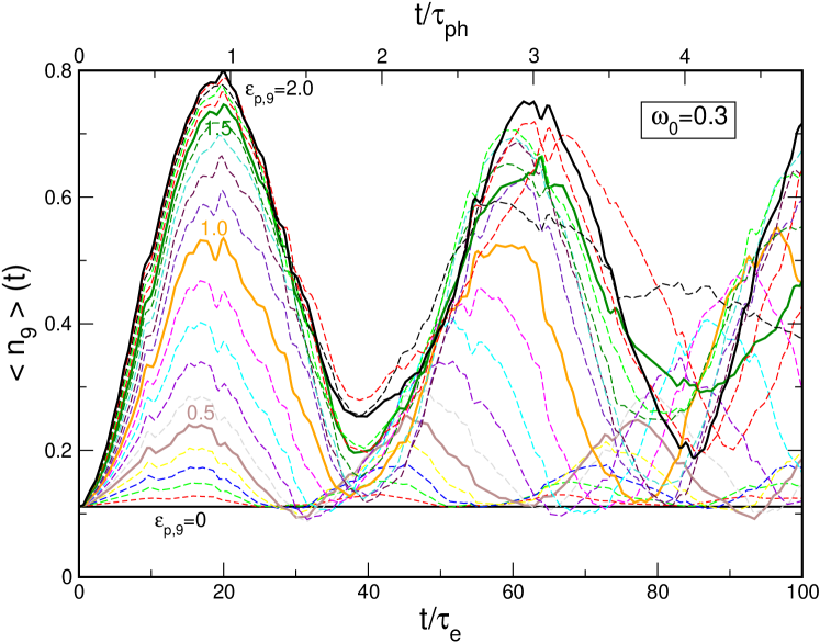
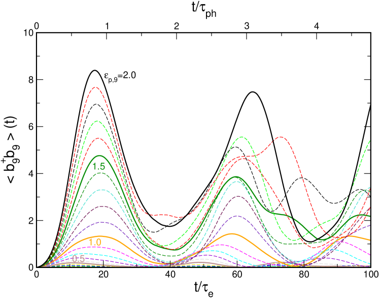
Figure 1: (Color online) Time dependence of the particle density (upper panel) and phonon number (lower panel) at the deformable “molecular crystal” site 9, starting out from the free-electron ground state of a 17 site chain with OBCs. The phonon frequency $\omega_{0}=0.3$. The EP coupling $\varepsilon_{p,9}$ is switched on at $t=0$, different curves belong to $\varepsilon_{p,9}$ values increased by 0.1. In the numerical calculations we take into account up to $M=100$ phonons, $N_{\rm C}=10$ Chebyshev moments, and use a time step $\Delta t/\tau_{e}=0.01$.

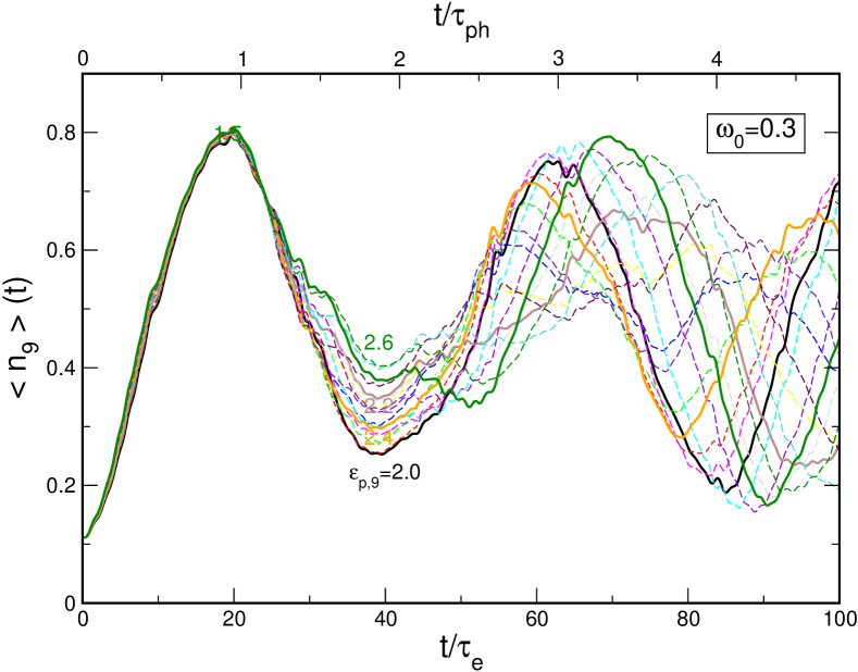
Figure 2: (Color online) Time dependence of the particle density (upper panel) and phonon number (lower panel) at molecular crystal site 9 in the intermediate EP coupling adiabatic regime. The initial state is the same as in Fig. 1; $\varepsilon_{p,9}$ now is increased in steps of 0.04.

Figure 1 illustrates the time evolution of the particle density at the oscillatory site after the interaction quench for weak-to-intermediate EP couplings and phonon frequencies $\omega_{0}$ smaller than the electronic transfer integral $t_{0}$. We note that the electron is not uniformly spread over the lattice even at $t<0$ where $\varepsilon_{p,9}=0$ because of of the OBCs: $\langle n_{9}\rangle(0)=1/9$ is roughly twice the mean electron density 1/17.

After the local EP interaction is turned on the electron can couple to the molecular vibrations at site 9. The basic interaction process is the absorption and emission of a phonon by the electron with a simultaneously change of the electron state. At the same time the lattice is distorted locally. Such a lattice distortion may trap the charge carrier if the EP coupling is strong. As a result the local particle density is enhanced. Since the trapping potential itself depends on the carrier’s state, this highly non-linear feedback phenomenon is called “self-trapping”. Firsov (1975); Wellein and Fehske (1998) Figure 1 clearly shows an initial strong increase of the local particle density in time. Since the characteristic nearest-neighbor hopping time of a bare electron is $\tau_{e}$, all “electrons” initially moving toward the central site will reach this site within $t/\tau_{e}\leq 8$ (dealing with a single particle we actually thereby think of electronic contributions). This explains the small hump on the left shoulder of the first $\langle n_{9}\rangle$–increase at about $t/\tau_{e}\sim 8$. Electrons that move away from the central site will reach it after reflection at the boundaries within the time interval $8<t/\tau_{e}\leq 17$. So if the particle is held at the molecular site by the EP coupling, it is trapped to the greatest possible extent at about $t/\tau_{e}\sim 17$ (which almost coincides with the first maximum in $\langle n_{9}\rangle$ at $t_{\rm max}^{(1)}/\tau_{e}\simeq 20$). Self-evidently the maximum is enhanced as $\varepsilon_{p,9}$ increases.

When an electron reaches site 9 it can emit a phonon to lower its energy. The phonon period is $\tau_{ph}$. Hence, for the adiabatic regime discussed in Fig. 1, the phonon excited by the first arriving “part of the electron” is still present when the last part of the electron arrives (cf. the phonon time scale displayed in the graphs at the opposite $x$-axes). Because of this retardation effect the number of phonons at the molecular site 9 steadily increases and $\langle b_{9}^{\dagger}b_{9}\rangle~{}$ develops, for $\omega_{0}=0.3$, a maximum in time slightly before $\langle n_{9}\rangle$ reaches its maximum. As time proceeds further, the particle starts hopping further away from the oscillatory site (recall that the system is no longer in an eigenstate after the interaction quench) and $\langle n_{9}\rangle(t)$ decreases until the whole process recurs. Importantly, the particle density $\langle n_{9}\rangle(t)$ at its first mimium around $t_{\rm min}^{(1)}\sim 2t_{\rm max}^{(1)}\simeq 40\tau_{e}$ is substantially larger than at $t=0$ above the “critical” EP coupling $\varepsilon_{p,9}/2t_{0}\simeq 1$. This gives a first indication that indeed a polaron is formed at site 9, in contrast to the weak EP coupling case.

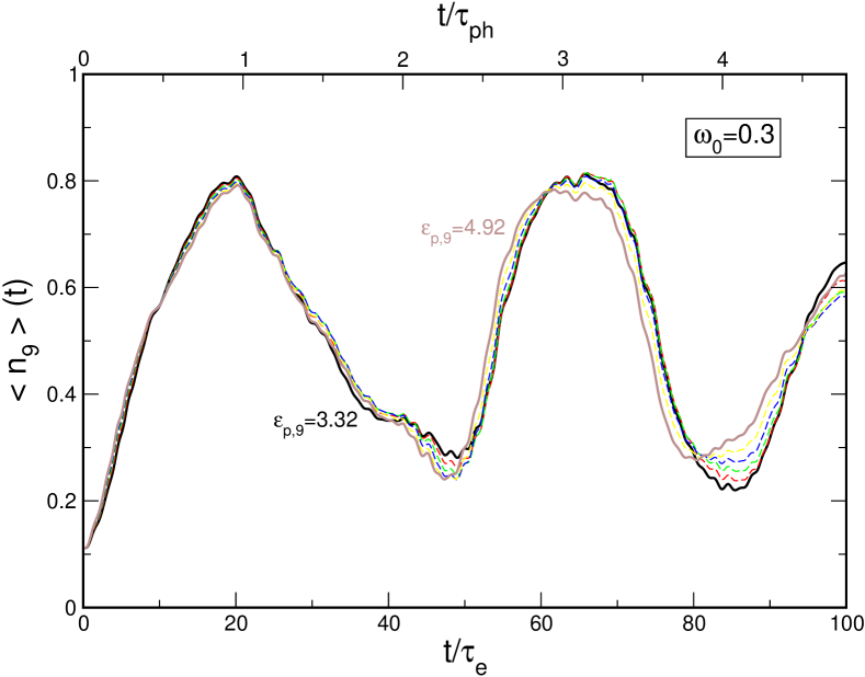
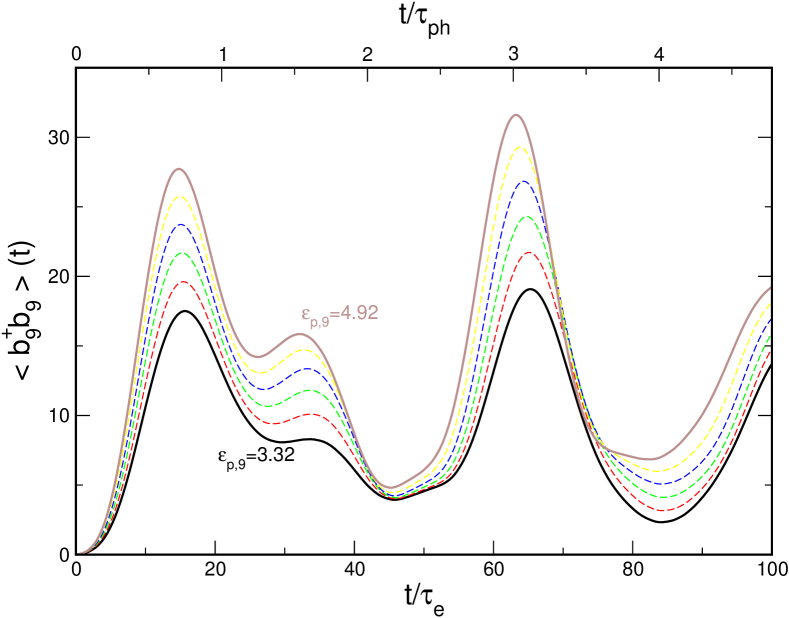
Figure 3: (Color online) Time dependence of the particle density (upper panel) and phonon number (lower panel) at site 9 in the strong EP coupling adiabatic regime. Initial state as in Fig. 1; $\varepsilon_{p,9}$ is increased in steps of 0.32.

Figures 2 and 3 demonstrate that at larger EP couplings the particle density at the oscillatory site 9 evolves in almost the same manner for a relatively long time span. This especially holds for the strong-coupling case displayed in Fig. 3, where every incoming electron sticks to the molecular site. Thereby the total phonon number increases with increasing $\varepsilon_{p,9}$. Then the interesting question is, of course, whether (or to what extent) the excited phonons are incorporated in the polaronic quasiparticle or rather will be uncorrelated. In our case, where the EP coupling acts on a single site only, the electron can not carry a phonon cloud away (this–more realistic–situation will be investigated in the subsequent two sections). Nevertheless we can address this question by analyzing the phonon distribution function, $|c_{m}|^{2}(t)$ with $\sum_{m=0}^{M}|c_{m}|^{2}(t)=1$, yielding the weight of the $m$-phonon contribution in the wave function $|\psi(t)\rangle$. Jeckelmann and Fehske (2007)

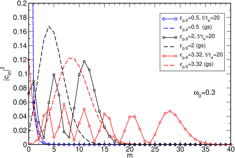
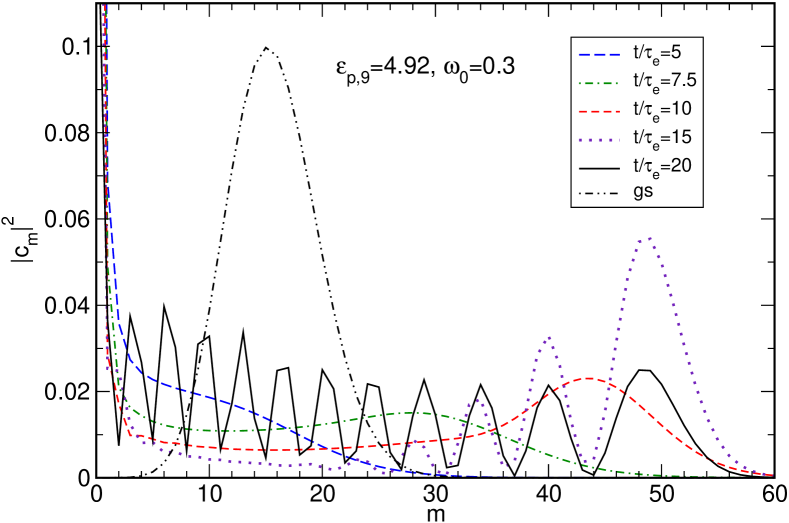
Figure 4: (Color online) Contribution of the $m$-phonon state to $|\psi(t)\rangle$ at different times $t$ (given in units $\tau_{e}$). Results for various $\varepsilon_{p,9}$ were compared to the phonon distribution function of the system’s ground state ($\varepsilon_{p,9}>0\forall\,t$, no interaction quench). The phonon frequency is $\omega_{0}=0.3$.

Figure 4 gives $|c_{m}|^{2}(t)$ for different EP interaction strengths, ranging from weak to strong couplings. For comparison, the corresponding phonon distribution functions of the stationary ground states (where $\varepsilon_{p,9}>0$ $\forall t$) is shown. At small $\varepsilon_{p,9}$, $|\psi(t)\rangle$ basically is a zero-phonon state at any time. As a matter of course a few phonons will be emitted but immediately after will be reabsorbed as the particle passes the molecular site. Therefore, no long-living lattice distortion appears that might trap the carrier. The situation dramatically changes as $\varepsilon_{p,9}$ exceeds the critical coupling strength for polaron formation. Now the phonon distribution of the ground state is Poisson distributed with maxima at about 4 ($\varepsilon_{p,9}=2$), 9 ($\varepsilon_{p,9}=3.32$), and 15 ($\varepsilon_{p,9}=4.92$). $|\psi(t=20\tau_{e})\rangle$ is a multi-phonon state as well. Since $\omega_{0}$ is rather small, an adiabatic potential (energy) surface emerges that retains the incoming electron contributions so that the formation of an adiabatic Holstein polaron Holstein (1959); Wellein and Fehske (1998) can occur. The initial energy of our system ($E_{0}=-1.9696$), however, does not allow the particle to access the polaronic ground state having $E_{0}(\varepsilon_{p,9}=2)=-2.521$, $E_{0}(3.32)=-3.628$, and $E_{0}(4.92)=-5.126$. As can be seen from Fig. 4, the form of the phonon distribution function reflects the phonon distribution of excited displaced harmonic oscillator states, indicating that excited states of the polaron were realized instead. These states are known to be separated in energy by $\omega_{0}$. Fehske and Trugman (2007) Indeed, in going e.g. from $\varepsilon_{p,9}=3.32$ to $\varepsilon_{p,9}=4.92$ five additional phonons were created (all bound to the polaron), giving rise to a polaron excited state. Note that such kinds of phonon distributions were found for the Raman- and infrared-active intrinsic localized modes in quasi one-dimensional mixed-valence transition-metal complexes. Swanson et al. (1999)

Figure 5: (Color online) Electron densities on the one-dimensional chain at different times $t/\tau_{e}$. Initial state as before; $\omega_{0}=0.3$.

The lower panel of Fig. 4 yields some insight on the time scale that the polaron formation process takes place. Up to $t/\tau_{e}=10$ the electron radiates successive phonons which are still uncorrelated, however. Therefore all phonon states below a certain threshold are equally well represented in $|\psi(t)\rangle$. The zero-phonon state has a larger weight, of course, because parts of the electron still reside outside the molecular site. At about $t/\tau_{e}=15$ the phonons become correlated, i.e. they are increasingly tightly bound to the electron. This process is completed at $t/\tau_{e}\sim 20$.

In Fig. 5 we show snapshots of the electron density distribution along the whole chain at various points in time. We see that by increasing the EP interaction in such a way that the energy of the initial state matches one of the polaron excited states (starting out from the well-established polaronic state at $\varepsilon_{p,9}=3.32$, see Figs 3 and 4), the spatiotemporal variation of the various excited states is the same, even for very long times and away from the central molecular site (cf. the curves marked by squares, diamonds and circles for $\varepsilon_{p,9}=3.64$, 3.96 and 4.28, respectively). In contrast, if we choose an EP coupling which does not match the ground-state energy $E_{0}$ by lowering the polaron-level ladder, after a while the densities evolve quite differently [cf. data for $\varepsilon_{p,9}=3.80$ (stars)].

III.1.2 Anti-adiabatic regime

We next investigate the limit of large phonon frequencies. Now $\tau_{ph}$ is comparable or even smaller than $\tau_{e}$, which means that a phonon can be excited and re-absorbed instantaneously when the electron enters the molecular site. During this process the electron will become (partly) dressed by phonons, provided the EP interaction is sufficiently strong. In this case a non-adiabatic Lang-Firsov-type polaron is formed. Lang and Firsov (1962); Wellein and Fehske (1998) This will not happen in the weak EP coupling regime illustrated in Fig. 6. Because of the extremely large phonon energy, only very few phonons can be radiated by the electron (see lower panel). The molecular-site particle density shown in the upper panel is weakly modulated by the phonon emission-absorption processes on the time scale $\tau_{ph}$ and “oscillates” on a time scale related to the system size $N=17$ (within $t/\tau_{e}=17$ all electrons have visited the central site once). No retardation phenomena are observed (in contrast to Fig. 1). The dip around $t/\tau_{e}=10$ is because electrons continously leaving the dot and those arriving at this time mostly come from the boundary where the electron density at $t=0$ was very small. The situation becomes more complex as $\varepsilon_{p,9}$ increases and the electron at the molecular site will be partly dressed leading to stronger fluctuations of the phonon number.

Figure 6: (Color online) Time dependence of the particle density (upper panel) and phonon number (lower panel) at molecular crystal site 9 in the weak EP coupling anti-adiabatic regime. The phonon frequency $\omega_{0}=8$. The EP coupling is switched on at $t=0$; different curves belong to $\varepsilon_{p,9}$ values increased by 0.1.

At “intermediate” couplings $\varepsilon_{p,9}=10$ (note that $\varepsilon_{p,9}=10/\omega_{0}$ is of the order of one), the ground-state energy $E_{0}(10)=-10.1215$ and the system comes into “resonance” with the initial state (having $E_{0}\sim-2$) by exciting just one phonon (see Fig. 7). Since $g_{9}^{2}>1$ a polaron will evolve, i.e. the phonon is bound to the electron. The same happens at $\varepsilon_{p,9}=18$ ($E_{0}(18)=-18.0622$), but now two phonons will be excited and incorporated. There are two points worth mentioning. First, as the system oscillates on its $t/\tau_{e}=17$-period it can adjust far better in order to form a polaron at the sequent $t_{\rm max}$-points. Second, putting $\varepsilon_{p,9}$ only somewhat out of tune, both $\langle n_{9}\rangle$ and $\langle b_{9}^{\dagger}b_{9}\rangle$ are substantially reduced for all $t$, i.e. polaron formation is suppressed.

Figure 7: (Color online) Time dependence of the particle density (upper panel) and phonon number (lower panel) at the molecular crystal site 9 in the strong EP coupling anti-adiabatic regime.

In the strong EP coupling regime displayed in Fig. 8, the anti-adiabatic Lang-Firsov polaron has been fully developed. In this case the arriving electronic contributions stay at the molecular site for such a long time that $\langle n_{9}\rangle$ reaches 0.8. Note the increase of $t_{\rm max}^{(1)}$ as compared to Figs. 6 and 7 (in order to demonstrate that $t_{\rm max}^{(1)}$ is indeed determined by the system size we included results for a system with $N=21$ sites). The lower panel makes clear that now on average many more phonons ($\propto g_{9}^{2}$) were incorporated.

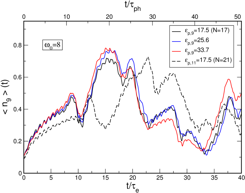
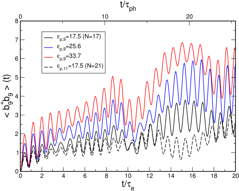
Figure 8: (Color online) Time dependence of the particle density (upper panel) and phonon number (lower panel) at the molecular crystal site 9 in the extremely strong EP coupling anti-adiabatic regime. The EP interaction is increased in steps of $\omega_{0}$. For $N=21$ the particle and phonon numbers are displayed at site 11.

The phonon distribution function shown in Fig. 9 corroborates this scenario. As for the adiabatic case (cf. Fig. 4), we observe a transition from an uncorrelated few-phonon state to a correlated multi-phonon polaron state. The phonon distribution function shows that $|\psi(t^{(1)}_{\rm max})\rangle$ corresponds to an excited polaron with two (four) bound phonons at $\varepsilon_{p,9}=18$ ($\varepsilon_{p,9}=33.7$).

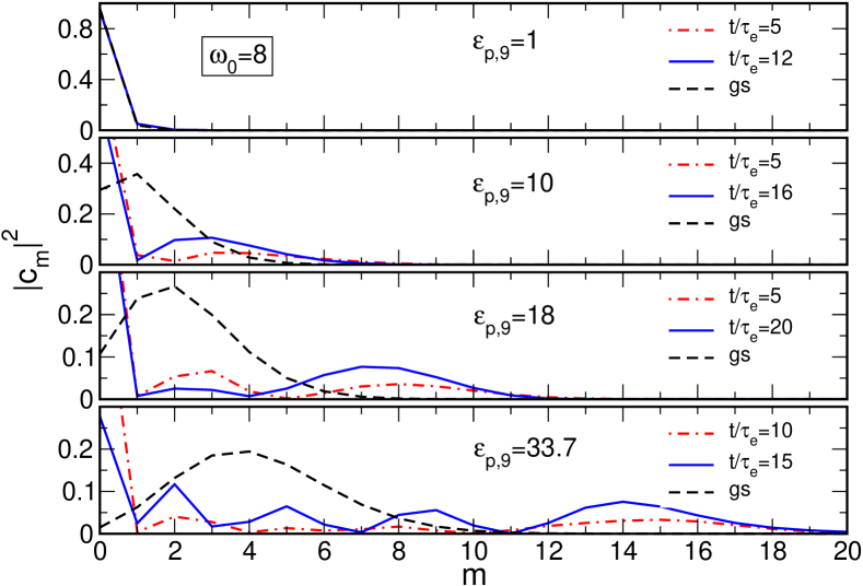
Figure 9: (Color online) Contribution of $m$-phonon states to $|\psi(t)\rangle$ at different EP couplings and points of time. Results were compared to the stationary phonon distribution function of the system’s true ground state. The phonon frequency is $\omega_{0}=8$.

III.2 Wave-packet injection

A bare electron injected into a quantum wire coupled to the lattice vibrations at every lattice site is another instructive example for the quantum dynamics of polaron formation. Ku and Trugman (2007) To this end, at $t=0$, we place a Gaussian wave packet of width $\sigma_{0}^{2}=3/\ln 10$ and momentum $K$ centered at site $l_{0}=4$,

$$|\psi(0)\rangle=A\sum_{l=1}^{7}{\rm e}^{\big{[}-\tfrac{(l-l_{0})^{2}}{2\sigma_{0}^{2}}\big{]}}{\rm e}^{{\rm i}K(l-l_{0})}c_{l}^{\dagger}|0\rangle\,,$$ (13)

and let it evolve ($A$ is a normalization constant to ensure $\langle\psi(0)|\psi(0)\rangle=1$). Again $\Delta_{i}=0$ $\forall i$.

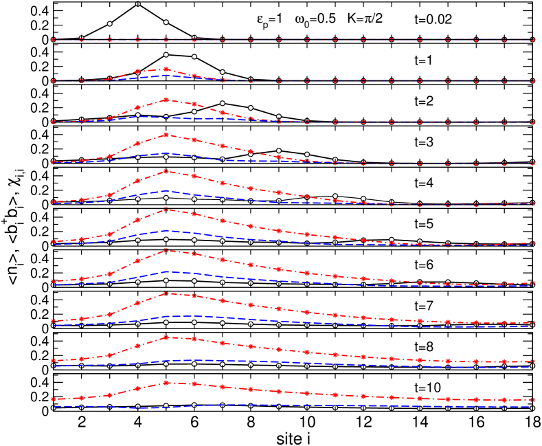
Figure 10: (Color online) Spatiotemporal evolution of a free electron Gaussian wave packet injected with wave vector $K=\pi/2$ at $t=0$ into an 18-site molecular crystal chain with PBCs. Model parameters are $\varepsilon_{p}=1$ and $\omega_{0}=0.5$. Displayed is the time evolution (in units of $\tau_{e}$) of the local particle densities $\langle n_{i}\rangle$ (black solid lines, open circles), phonon numbers $\langle b_{i}^{\dagger}b_{i}\rangle$ (red dot-dashed lines, stars) and local EP correlations $\chi_{i,i}$ (blue dashed lines).

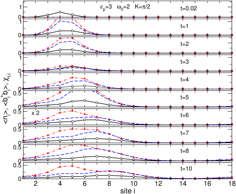
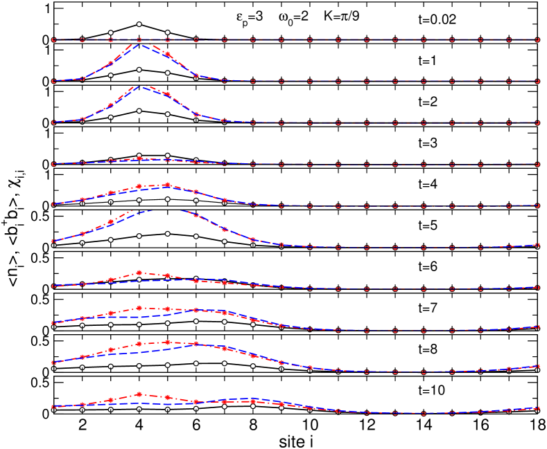
Figure 11: (Color online) Spatiotemporal evolution of a free electron Gaussian wave packet injected with wave vector $K=\pi/9$ (upper panels) and $K=\pi/2$ (lower panels) at $t=0$. Model parameters are $\varepsilon_{p}=3$ and $\omega_{0}=2$. Notations as in Fig. 10.

Figure 10 shows snapshots of the local particle densities $\langle n_{i}\rangle$ and phonon numbers $\langle b_{i}^{\dagger}b_{i}\rangle$ for intermediate EP couplings ($\varepsilon_{p}=1$ at all sites) and adiabatic phonon frequencies ($\omega_{0}=0.5$). In addition we included results for the on-site particle-phonon correlations

$$\chi_{i,i}=\langle n_{i}(b_{i}+b_{i}^{+})\rangle\,.$$ (14)

The particle injected at site 4 is launched to the right ($K=\pi/2$). Shortly after, the electron is not yet dressed and moves nearly as fast as a free particle (see black curves in the panels for $t/\tau_{e}=0.02$, 1, 2, and 3). Ku and Trugman (2007) At the same time the electron emits (creates) phonons along its path, in order to reduce its energy to near the bottom of the band. In view of the high initial energy $E_{0}(t=0)=0$ and an intermediate EP coupling strength most of the phonons radiated are uncorrelated and therefore continue to stay near the particle’s starting point. Nevertheless the particle drags some phonons with it and finally a (coherent) polaron wave packet is formed characterized by enhanced local particle-phonon correlations (see sites 5–7 in the panels for $t/\tau_{e}=6$–8; note that the polaronic quasiparticle moves with a reduced velocity Ku and Trugman (2007); Weiße and Fehske (2008)). Owing to the moderate EP coupling these signatures are rather weak, however, and are further smeared out when the polaronic wave packet dissolves in time.

As Fig. 11 shows, polaron formation becomes more pronounced at larger EP couplings ($\varepsilon_{p}=3$; note the different scale of the ordinate compared to Fig. 10), even if the phonon frequency is enhanced as well ($\omega_{0}=2$, non-adiabatic regime). The phonon distribution and enhanced on-site EP correlations indicate that more phonons are in the phonon cloud that travels with the particle. Thereby the polaron inertial mass is increased. Again some unbound phonons stay at the point where the particle takes off. While in the upper graph the particle is injected with an energy of about the phonon energy above the bottom of the band, its energy is much lower in the lower graph where $K=\pi/9$. This difference is mainly reflected in the number of unbound phonons; in both cases the polaronic quasiparticle emerges at about $t/\tau_{e}=8\ldots 10$ and shows the same characteristics afterwards.

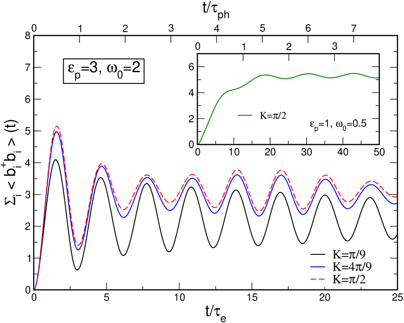
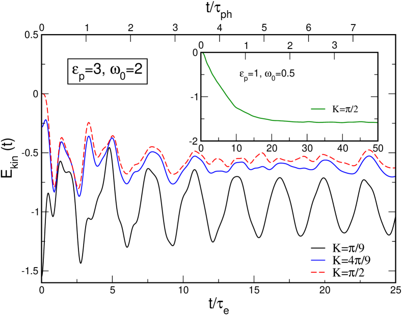
Figure 12: (Color online) Upper panel: Time dependence of the total number of phonons excited in the molecular crystal chain as the free electron wave packet evolves into a polaron. Lower panel: Time evolution of the kinetic energy part $E_{\rm kin}$.

Since the system is not in an eigenstate we expect to find (decaying) oscillations on the time scale of $\tau_{ph}$ in the process of polaron formation; at least if $\tau_{e}$ and $\tau_{ph}$ do not differ too much and the EP coupling is not too small. This is illustrated by Fig.  12, showing the variation in time of the total number of phonons in the system and of the kinetic energy part ,

$$E_{\rm kin}=-t_{0}\sum_{i}\langle c_{i}^{\dagger}c_{i+1}+{\rm H.c.}\rangle\,.$$ (15)

For $\omega_{0}=2$ (main panels) these oscillations can be clearly detected in both quantities. The kinetic energy $E_{\rm kin}(\varepsilon_{p}=3,\omega_{0}=2)=-1.316$ for the ground state of a polaronic system having the same parameters. We find that this value can be much better (periodically) approached, injecting a particle with lower energy, i.e. $K=\pi/9$. The minima in $E_{\rm kin}$ are reached when the particle has absorbed some phonons. Afterward the particle radiates the phonons again and its kinetic energy increases. The oscillations are weaker at $K=\pi/2$. While the wave vector of the injected wave packet (13) is a continuous variable, finite chains with PBC have only a finite set of “allowed” $K$ vectors. Because $\pi/2$ is not an allowed wave vector of the periodic 18-site system, we included data for $K=4\pi/9$ (located next to $K=\pi/2$) as well, but—as expected—the results do not change qualitatively. The insets give the total phonon number and kinetic energy for the parameters of Fig. 10, i.e. for the adiabatic case. Here we can clearly distinguish two regimes: until $t/\tau_{e}\sim 6$ many unbound phonons were created to lower the particle’s total energy; then polaron formation sets in and the particle attains a kinetic energy close to the polaron’s ground-state kinetic energy $E_{\rm kin}(\varepsilon_{p}=1,\omega_{0}=0.5)=-1.823$.

III.3 Polaron tunneling

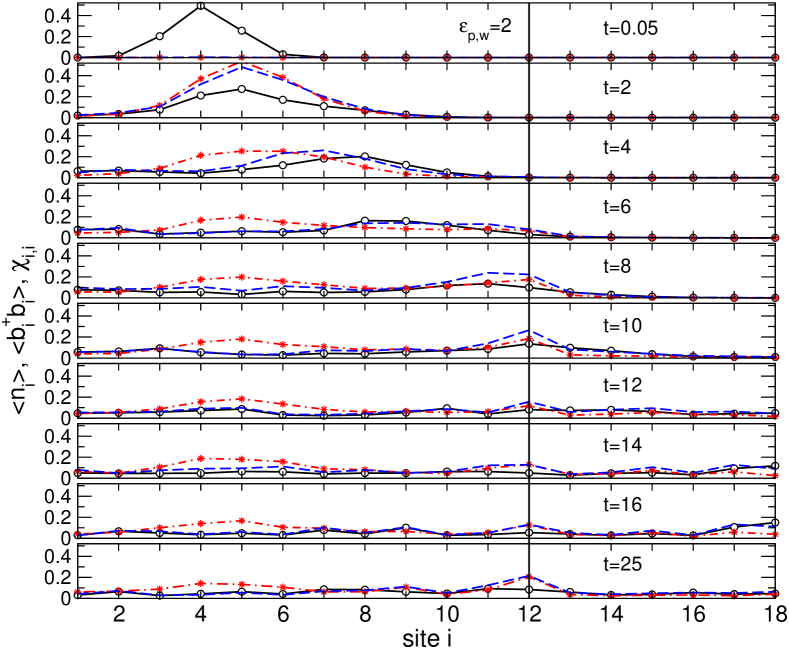
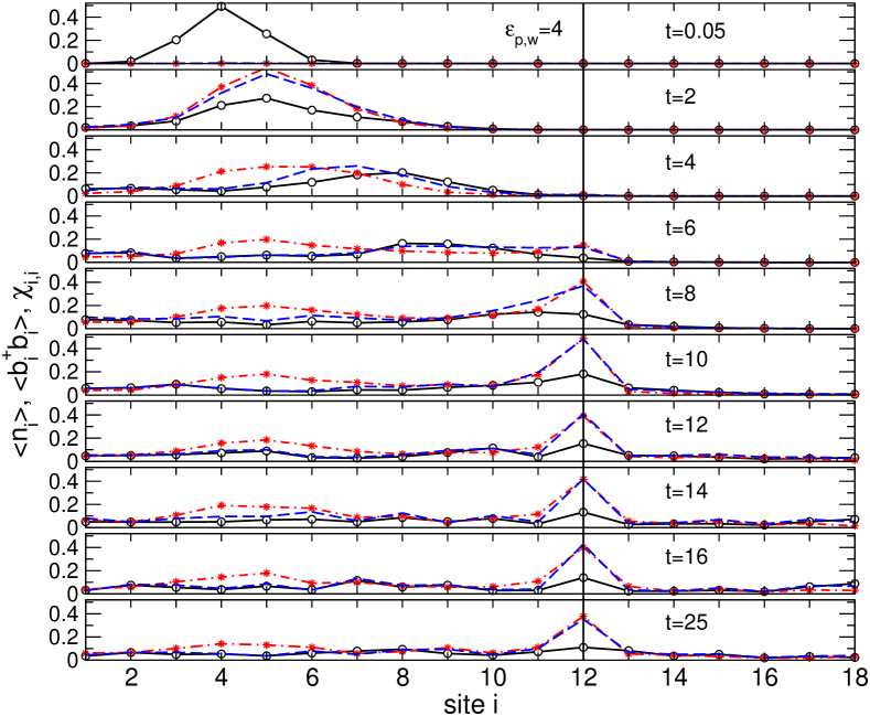
Figure 13: (Color online) Quantum dynamics of polaron formation and polaron tunnelling through a potential barrier $\Delta_{12}=\Delta_{w}=2$. Model parameters are $\varepsilon_{p}=1$, $\omega_{0}=2$. The barrier or quantum dot is located at site 12 and has a total EP coupling $(\varepsilon_{p}+\varepsilon_{p,w})$. OBCs were used at sites 1 and 18. Notation is the same as in Fig. 11. For further explanation see text.

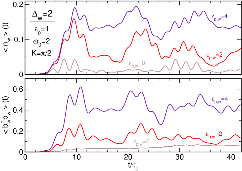
Figure 14: (Color online) Time dependence of the particle density (upper panel) and phonon number (lower panel) at the site of the wall.

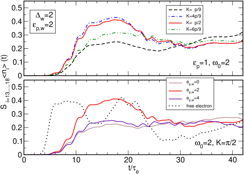
Figure 15: (Color online) Cumulated particle density to the right of the potential wall at different wave vectors $K$ (upper panel) and various EP couplings $\varepsilon_{p}$ (lower panel), for the setup of Fig. 13.

Finally we investigate the tunneling of a polaronic quasiparticle through a potential barrier $\Delta_{12}\equiv\Delta_{w}=2$ (quantum wall or dot), with additional EP interaction $\varepsilon_{p,12}\equiv\varepsilon_{p,w}$. For $i\neq 12$ we fix $\Delta_{i}=0$. The other model parameters are choosen to be $\varepsilon_{p}=1$ and $\omega_{0}=2$. In the numerics we account for all states with up to $M\leq 11$ phonons and have checked that in the ground state the weight of basis states containing exactly $M=11$ phonons is, for the largest $\varepsilon_{p,w}$, less than $10^{-5}$.

The wave packet injected has energy $E_{0}(0)=0$ and moves to the right with $K=\pi/2$ (see Fig. 13). We apply OBC, so the particle cannot avoid the barrier coming from behind. The upper graph describes the situation with a barrier at site 12 only. After the polaron is formed at $t/\tau_{e}\sim 6$ it hits the quantum wall at $t/\tau_{e}\sim 8-10$ and there is mostly reflected. Besides this backscattered particle current a minor part of the particle tunnels through the barrier, thereby partly stripping and recollecting its accompanied phonons (cf. Fig. 15 below). Envisaging a vibrating molecular quantum dot located at site 12 (middle panel), an additive EP interaction $\varepsilon_{p,w}$ leads to a local polaronic level shift that softens the barrier. As a result the particle is transmitted to a much greater extent than in the former case (compare the results for $t/\tau_{e}=14-16$). If the quantum dot possess a very strong EP interaction the polaron digs at the dot site and stays there for a long time (see lower panel). Then of course both the reflected and transmitted particle current is low.

Figure 14 gives the temporal variation of particle density and phonon number at the quantum wall/dot site. Obviously the phonons somewhat lag behind the electron (retardation effect). During the tunneling process the phonon number strongly fluctuates. The $\varepsilon_{p,w}=4$ curve clearly signals the self-trapping of the electron at the dot site. The second bump-series is due to electronic contributions retaining after being reflected at the system’s boundary (site 18).

The total transmitted electron density is displayed in Fig. 15 for $\varepsilon_{p,w}=\Delta_{w}$ and various momenta of the injected wave packet (upper panel) as well as for different $\varepsilon_{p,w}$ at $K=\pi/2$ (lower panel). Of course a higher initial energy enhances the transmission through the tunnel barrier (compare the $K=\pi/2$ and $K=\pi/9$ curves). The lower panel first of all shows the time delay of the polaron in reaching the barrier compared to a free particle (dotted line). More notably, we observe that for $\varepsilon_{p,w}=2$ the transmission is as high as for free particles, despite the fact that the particle is dressed by phonons in a significant way. Note that the dimensionless EP coupling parameters at the dot site are $3/2t_{0}$ and $g_{12}^{2}=1.5$. This points toward the importance of vibration-mediated tunneling processes (doorway vibrons). Fehske et al. (2008)

IV Summary

In this work, we have presented an efficient numerical method to calculate the time evolution of the many-body wave function of an interacting electron-phonon system. The approach is based on Chebyshev moment expansion, applied to the time evolution operator. We focused on the process of small polaron formation in finite low-dimensional quantum structures described by a generalized Holstein Hamiltonian. Both electron and phonon quantum dynamics were treated exactly.

We first started from a non-interacting ground state and analyzed the real-time dynamics of the particle density and phonon number after a sudden switching-on of the electron-phonon coupling at a single oscillatory (molecular quantum dot) site. As a consequence of this interaction quench the originally free particle can be trapped at the “impurity” site after a while. The self-trapping process differs in nature for the adiabatic and anti-adiabatic regimes of small and large phonon frequencies, respectively. In the former case, where the phonons are slow and retardation effects play an important role, a static lattice distortion evolves that causes an effective attractive potential for the electron. As a result a Holstein polaron is formed. In the latter case phonons can follow the electron motion almost instantaneously. Hence we observe very fast phonon emission and re-absorption processes, which—at large EP interaction strengths—give rise to a dynamical dressing of the charge carrier that enhances the particle’s mass and finally leads to its immobilization. In both cases the phonon distribution function signals the existence of excited bound polaron-phonon states. Since our initial state is not an eigenstate of the interacting system, we observe the phenomenon of recurrence at later times.

Next we launched a free-electron Gaussian wave packet in a one-dimensional system, subjected to EP coupling at every site. The injected bare particle is found to radiate phonons to lower its energy to near the bottom of the band. Thereforre part of the phonons stay near the electron’s starting point and—if the EP coupling is sufficiently strong—another part of the phonons will be embedded in a phonon cloud attached to the (moving) particle. The latter polaron quasiparticle formation process takes a period of time that depends on the characteristic electron and phonon times scales, the EP interaction strength, and the initial conditions in a very sensitive way. We agree with the findings of previous work Ku and Trugman (2007) that the question of how long it takes a polaron to form, has no simple answer, because there are multiple time scales in the dynamics.

In the last part we investigated the transmission of a polaron through a quantum wall or vibrating quantum dot. Depending on the barrier height to electron-phonon interaction strength ratio, and the characteristic electron and phonon times scales, we found opposed behaviors: strong reflection; phonon-mediated tunneling; and intrinsic localization of the polaron. Most notably we showed that if the polaronic level lowering just compensates the repulsive dot potential and the electron and phonon time scales are comparable, a rather heavy small polaron, regardless of its phonon cloud, tunnels like a free electron, On the other hand, if there is a mismatch between both quantities , we observe strong phonon fluctuations at the dot site and transport through the quantum dot becomes significantly suppressed. This might motivate further investigations of deformable quantum dot systems, e.g. with respect to applications as a current switch.

In conclusion, we have demonstrated that polaron formation is a subtle non-linear dynamical process which is affected by multiple time/energy scales. The proposed long-time Chebyshev expansion method—in combination with exact diagonalization techniques—is capable of addressing such complex problems, which raises the expectation that our approach can also be used to study the time-evolution of quasiparticles in more general situations.