Low-temperature electrical resistivity in paramagnetic spinel LiV₂O₄

Abstract

The 3$d$ electron spinel compound LiV₂O₄ exhibits heavy fermion behaviour below 30K which is related to antiferromagnetic spin fluctuations strongly enhanced in an extended region of momentum space. This mechanism explains enhanced thermodynamic quantities and nearly critical NMR relaxation in the framework of the selfconsistent renormalization (SCR) theory. Here we show that the low-$T$ Fermi liquid behaviour of the resistivity and a deviation from this behavior for higher $T$ may also be understood within that context. We calculate the temperature dependence of the electrical resistivity $\rho(T)$ assuming that two basic mechanisms of the quasiparticle scattering, resulting from impurities and spin-fluctuations, operate simultaneously at low temperature. The calculation is based on the variational principle in the form of a perturbative series expansion for $\rho(T)$. A peculiar behavior of $\rho(T)$ in LiV₂O₄ is related to properties of low-energy spin fluctuations whose $T$-dependence is obtained from SCR theory.

I Introduction

The metallic vanadium oxide LiV₂O₄ has attracted much attention after a heavy fermion behavior in this 3$d$-electron system was discovered.Kondo97 ; Johnston00 ; Kondo99 The cubic spinel LiV₂O₄ has the pyrochlore lattice of vanadium ions (in the mixed valence state V^3.5+) and shows metallic conduction and no long-range magnetic ordering for any measured temperatures at ambient pressure. So far the origin of the heavy fermion quasiparticle formation observed in this compound for $T<10$K remains to be a controversial subject, however, effects of electronic correlations and the geometrical frustration of the pyrochlore lattice are supposed to be key aspects of the problem.

The quasiparticle mass enhancement is expected when a metallic system is driven by strong electron correlations to a vicinity of a charge and/or spin phase transition at low $T$. In that case, the charge/spin disordered ground state on the metallic side of the transition in the strongly correlated system LiV₂O₄ is sustained because a long-range order with a particular ordering (critical) wave vector ${\bf Q}_{c}$ is prevented by the geometrical frustration. Expressed differently, the system cannot choose a unique wave vector of an ordered structure which minimizes the free energy. Instead, it is frustrated between different structures with different critical wave vectors ${\bf Q}_{c}$’s and equally low free energy. For instance, low energy spin fluctuations are expected to be present in a very large region of momentum space which is the signature of frustrated itinerant magnetism. This is in contrast to non-frustrated systems where the fluctuations are confined to the immediate vicinity of a unique incipient ordering vector.

This scenario for frustrated itinerant magnetism was recently investigated in detail for LiV₂O₄ by present authors.Yushankhai07 . An analysis of inelastic neutron scattering (INS) measurementsKrimmel99 ; Lee01 ; Murani04 and calculations of the dynamic spin susceptibility allowed us to suggest the location of the paramagnetic spinel LiV₂O₄ close to a magnetic instability. This was achieved by developing the RPA theory of spin fluctuations based on ab-initio band structure calculations and an on-site Coulomb interaction of 3$d$ electrons. Close to the critical value of the interaction strength, low energy spin fluctuations develop throughout a large shell in momentum space. They may be mapped to an effective low energy paramagnon model which describe low-temperature INS resultsKrimmel99 ; Lee01 ; Murani04 accurately. From the comparison at $T\to$ 0, the parameters of the model (peak energy, weight and extension in momentum space) are fixed. Using the selfconsistent renormalization (SCR) theory,Moriya73 ; Hasegawa74 ; Moriya85 which includes mode-coupling of spin fluctuations, the finite $T$ properties of INS spectral shapes, uniform and staggered susceptibility, as well as NMR relaxation rate, have been explained Yushankhai07 ; Yushankhai08 ; Yushankhai2008 . From this analysis we concluded that LiV₂O₄ can be regarded as a nearly antiferromagnetic (AFM) metal and its unusual low-$T$ properties have to be related to a peculiar structure of the paramagnetic ground state with strongly degenerate low-energy (slow) AFM spin fluctuations.

In the present study, our main concern is to explain the low-temperature, $T<$ 40K, electrical resistivity $\rho(T)$ measured on single crystals of LiV₂O₄ and reported by Takagi et al.Takagi99 and Urano et al.Urano00 . A Fermi-liquid behavior $\rho(T)\sim T^{2}$ for $T<$ 2K and a more slow increase of $\rho(T)$ for higher temperatures were found. MeasurementsTakagi99 ; Urano00 revealed a noticeable change in physical properties of LiV₂O₄ for $T>$ 40K, including a Curie-Weiss magnetic susceptibility $\chi(T)$ and a highly incoherent transport, which is, however, beyond the scope of present theory. In our approach we will use the effective low energy paramagnon model for spin fluctuations whose parameters are completely fixed by the comparison with INS. Only two more pheonomenological parameters characterising the impurity and paramagnon scattering mechanism will be needed.

From an analysis of the optical reflectivity and conductivity measurements, Jönsson et al.Jonsson07 and Irizawa et al.Irizawa10 inferred that the conducting electron system in LiV₂O₄ at ambient pressure is located close to a correlation-driven insulating state. Under the applied external pressure,Irizawa10 the system undergoes a metal-insulator transition accompanied with a charge ordering and a structural lattice distortion in the insulating phase. The observed complicated phase transformation display properties different from those expected from a first-order phase transition or a conventional metal-insulator transition. We note that because of quarter-filling of the electronic $t_{2g}$ bands in LiV₂O₄, electron correlations due to inter-site Coulomb repulsion have to play an essential role in the observed transition.Yushankhai05 Under such conditions, a microscopic mechanism for the heavy quasiparticle formation on the metallic side of the transition has to be clarified. However, in the present analysis which is concerned with resistivity under ambient pressure the effect of inter-site Coulomb interaction and a slowing-down of charge fluctuations will not be included.

It was realized some time ago that the calculation of low-$T$ transport properties in nearly AFM metals is a rather subtle issue. Hlubina95 ; Rosch99 ; Rosch00 In clean systems with a peculiar AFM ordering vector ${\bf Q}_{AFM}$ the quasiparticle scattering by quantum-critical spin fluctuations is strongly anisotropic. The strongest scattering occurs near the ”hot spots” of the Fermi surface (FS) connected by ${\bf Q}_{AFM}$ and the main contribution to the electrical conductivity is due to quasiparticles from the ”cold region” of the FS. In that case, if the system is at some distance from the AFM quantum critical point, the low-$T$ scattering rates are proportional to $T^{2}$ and the Fermi-behavior $\rho(T)-\rho_{imp}\sim T^{2}$ is realized. As was first pointed out by Rosch,Rosch99 ; Rosch00 if a small amount of disorder is present, an interplay of strongly anisotropic scattering due to critical spin fluctuations and an isotropic impurity scattering may complicate the picture producing several different regimes for $\rho(T)-\rho_{imp}\sim T^{\alpha}$ with the exponent between 1 $\leq\alpha\leq$ 2 in the low-$T$ region.

To describe temperature-dependent electrical resistivity in LiV₂O₄, we suggest that quasiparticles are scattered by AFM spin fluctuations almost equally strongly over the FS and effects of anisotropy are weak. This is related to a peculiar distribution of dominant AFM spin fluctuations with ordering vectors ${\bf Q}_{c}$’s forming a largely isotropic dense manifold in ${\bf k}$ space in this compound.Yushankhai07 Low-temperature evolution of interacting spin fluctuations in LiV₂O₄ can be successfully described within the SCR formalism as presented in our previous studies.Yushankhai08 ; Yushankhai2008 As explained in Ref.Moriya85, , the set of model parameters of the SCR theory were obtainedYushankhai08 from neutron scattering dataKrimmel99 ; Lee01 ; Murani04 and used to describeYushankhai2008 the temperature and pressure evolution of the spin-relaxation rate $1/T_{1}T$ observed in the NMR measurementFujiwara04 of the low-$T$ spin dynamics in LiV₂O₄. In this work, the theory is extended and applied to give an explanation of the low-$T$ electrical resistivity $\rho(T)$ in this compound.Takagi99 ; Urano00

II Variational principle for ${\bf\rho(T)}$: general consideration.

As follows from experimental observations,Kondo97 ; Johnston00 ; Kondo99 ; Takagi99 ; Urano00 the concept of the Fermi quasiparticles for charge carriers in the metallic spinel LiV₂O₄ is valid for sufficiently low temperatures, $T<$ 30 K. In this regime, we assume that the dominant scattering processes are given by low-energy AFM spin fluctuations and impurities. In the linear response theory, in an applied electric field $\bf E$ the quasiparticle distribution function $f_{\bf k}$ is linearized around the equilibrium Fermi distribution $f^{0}_{\bf k}$ according to $f_{\bf k}=f^{0}_{\bf k}-\Phi_{\bf k}df^{0}_{\bf k}/d\epsilon_{\bf k}$. The electronic transport can be found from the Boltzmann equation

$$-e({\bf Ev_{k}})\frac{df^{0}_{\bf k}}{d\epsilon_{\bf k}}=\sum\limits_{\bf k^{\prime}}W_{\bf kk^{\prime}}\Phi_{\bf k^{\prime}}.$$ (1)

The scattering operator $W_{\bf kk^{\prime}}$ can be expressed through the total equilibrium transition probability ${\mathcal{P}}_{\bf kk^{\prime}}={\mathcal{P}}_{\bf kk^{\prime}}^{imp}+{\mathcal{P}}_{\bf kk^{\prime}}^{sf}$ as ($k_{B}=\hbar=1$):

$$W_{\bf kk^{\prime}}=\frac{1}{T}\left(\delta_{\bf kk^{\prime}}\sum\limits_{\bf k^{\prime\prime}}{\mathcal{P}}_{\bf kk^{\prime\prime}}-{\mathcal{P}}_{\bf kk^{\prime}}\right),$$ (2)

provided the spin fluctuations are in thermal equilibrium, i.e., there is no drag effect.

For the elastic impurity scattering one has

$${\mathcal{P}}_{\bf kk^{\prime}}^{imp}=2\pi n_{i}|T_{\bf kk^{\prime}}|^{2}\delta(\epsilon_{\bf k}-\epsilon_{\bf k^{\prime}})f^{0}_{\bf k}(1-f^{0}_{\bf k^{\prime}}).$$ (3)

To a sufficiently good approximation, the $T$-matrix in Eq.(3) is frequently assumed to be a constant $|T_{\bf kk^{\prime}}|^{2}\approx V_{imp}^{2}$ and $n_{i}V_{imp}^{2}$, where $n_{i}$ is the impurity density, is regarded as a free parameter to be chosen so as to give a realistic value of the measured residual resistivity $\rho_{imp}$. We avoid this approximation and treat below matrix elements of ${\mathcal{P}}_{\bf kk^{\prime}}^{imp}$ generally.

For the spin-fluctuation ($sf$) scattering one hasUeda75 ; Ueda77 ; Hlubina95 ; Rosch00

$${\mathcal{P}}_{\bf kk^{\prime}}^{sf}=3J_{sf}^{2}f^{0}_{\bf k}(1-f^{0}_{\bf k^{\prime}})[n(\epsilon_{\bf k}-\epsilon_{\bf k^{\prime}})+1]\mbox{Im}\chi\left({\bf k}-{\bf k^{\prime}},\epsilon_{\bf k}-\epsilon_{\bf k^{\prime}}\right),$$ (4)

where $n(\epsilon)$ is the Bose distribution function, $\chi\left({\bf q},\epsilon\right)$ is the dynamical spin susceptibility describing the low-$T$ paramagnetic state of LiV₂O₄ and $J_{sf}$ is an effective coupling constant which is the second free parameter. It is worth emphasizing that in the present study the other parameters of the phenomenological SCR theory determining the behavior of $\chi\left({\bf q},\epsilon\right)$ are considered to be known and fixed from a fit to the data of inelastic neutron scattering measurement Krimmel99 ; Lee01 ; Murani04 on LiV₂O₄, as discussed in Ref.Yushankhai08, .

Following the standard notationZiman60 , the Boltzmann equation (1) can be rewritten in the form $X_{\bf k}=\sum\nolimits_{\bf k^{\prime}}W_{\bf kk^{\prime}}\Phi_{\bf k^{\prime}}$. Then, the electrical resistivity can be obtained by minimizing a functionalZiman60

$$\rho[\Phi]=min\left[\frac{\langle\Phi,W\Phi\rangle}{|\langle\Phi,X(E=1)\rangle|^{2}}\right].$$ (5)

Here, $E=1$ means the unit electrical field and the scalar product of two functions $\Phi_{\bf k}$ and $\Psi_{\bf k}$ is defined as $\langle\Phi,\Psi\rangle=\sum\nolimits_{\bf k}\Phi_{\bf k}\Psi_{\bf k}$. In fact, in Eq.(5) the ${\bf k}$-integration over the actual FS is implied, which follows from the property of the scattering operator $W_{\bf kk^{\prime}}$ and the explicit form of $X_{\bf k}=e({\bf Ev_{k}})(-df^{0}_{\bf k}/d\epsilon_{\bf k})$.

A way to search for a variational solution of Eq.(5) for the deviation function $\Phi_{\bf k}$ is to expand it in a set of the Fermi-surface harmonics (FSH) $\phi_{L}(\bf k)$:

$$\Phi_{\bf k}=\sum_{L}\eta_{L}\phi_{L}(\bf k),$$ (6)

where $\eta_{L}$ are variational parameters and $L$ is a convenient composite label that includes numbering of different sheets of the FS in LiV₂O₄. The FSH’s are definedAllen76 ; Allen78 as polynomials of the Fermi-velocity Cartesian components $v_{\bf k}^{\alpha}$. That is, for each integer $N\geq 0$ one has to construct $(N+1)(N+2)/2$ polynomials $(v_{\bf k}^{x})^{l}(v_{\bf k}^{y})^{m}(v_{\bf k}^{z})^{n}$ with $l,m,n\geq 0$ and $l+m+n=N$, and orthonormalize them on the actual FS, $\langle\phi_{L^{\prime}},\phi_{L}\rangle=\delta_{L^{\prime}L}$. The resulting polynomials forming a complete set $\{\phi_{L}(\bf k)\}$ of basis functions are classified according to different irreducible representations $\Gamma$ of the lattice symmetry point group. In general, for a given $\Gamma$ there are subsets of different functions, $\{\phi_{L}^{r}(\bf k)\}$, $\{\phi_{L}^{s}(\bf k)\}$, etc., which transform according to the same $\Gamma$. Then, for any pair of partner functions, $\phi_{L^{\prime}}^{r}(\bf k)$ and $\phi_{L^{\prime\prime}}^{s}(\bf k)$, belonging to different subsets, but transforming according to the same row of $\Gamma$, one has $\langle\phi_{L^{\prime}}^{r},W\phi_{L^{\prime\prime}}^{s}\rangle\not=0$. The other off-diagonal matrix elements of the scattering operator $W_{\bf kk^{\prime}}$, including those connecting different irreducible representations, vanish by symmetry arguments and, hence, the scattering operator has a block-diagonal form (see the discussion by AllenAllen76 and references therein).

A minimum of $\rho[\Phi]$ is achieved in the class of odd functions, $\phi_{L}(-{\bf k})=-\phi_{L}({\bf k})$; only these basis functions are included in the expansion (6). Recalling the cubic symmetry of the LiV₂O₄ lattice structure, we assume without loss of generality that the applied electric field points in the ${\bf x}$ direction, which immediately distinguishes one of the first-order FSH’s: $\phi_{1x}({\bf k})=v_{{\bf k}}^{x}/\langle(v_{\bf k}^{x})^{2}\rangle^{1/2}$, where $\langle(v_{\bf k}^{x})^{2}\rangle^{1/2}$ is for the root-mean-square on the Fermi surface.

A general strategy in describing the physical resistivity $\rho(T)$ as a solution of the variational equation (5) in most of the metallic systems, including those with complicated electronic band structure, is to truncate the expansion (6) by keeping in it only a few of FSH’s. Following the common practice, one may start the analysis with the lowest, first-order variational solution, $\Phi_{\bf k}^{(0)}\sim\phi_{1x}({\bf k})$, which is a fairly good approximation provided the anisotropic effects of the quasiparticle scattering are weak. As usual, here the anisotropy of the scattering operator $W_{\bf kk^{\prime}}=W_{\bf kk^{\prime}}^{imp}+W_{\bf kk^{\prime}}^{sf}$ means that the transition probabilities depend not only on the mutual angle between the momenta ${\bf k}$ and ${\bf k^{\prime}}$, but also on their position with respect to the crystallographic axes. Anisotropic effects, as well as a complexity of the actual FS, can be partially caught in the calculations by keeping in the expansion (6) a selected number of higher-order FSH’s.

To go beyond the lowest-order solution for $\rho[\Phi]$ in the simplest manner, the following approximate assumption can be made: the off-diagonal matrix elements $W_{LL^{\prime}}=\langle\phi_{L},W\phi_{L^{\prime}}\rangle$ are small compared to diagonal ones, $W_{LL}$ and $W_{L^{\prime}L^{\prime}}$. Then, the variational solution to Eq.(5), being written in the familiar formZiman60 as $\rho^{-1}=X_{1}^{2}\langle\phi_{1x},W^{-1}\phi_{1x}\rangle$, where $X_{1}=\langle\phi_{1x},X\rangle$, can be expanded in a perturbation seriesAllen78

$$\rho\approx\frac{1}{X_{1}^{2}}W_{1x,1x}\left[1-{\sum_{L}}^{\prime}\frac{W_{1x,L}W_{L,1x}}{W_{1x,1x}W_{LL}}+{\sum_{LL^{\prime}}}^{\prime}\frac{W_{1x,L}W_{LL^{\prime}}W_{L^{\prime},1x}}{W_{1x,1x}W_{LL}W_{L^{\prime}L^{\prime}}}-...\right],$$ (7)

where the primes on the sums means that the terms with $L,L^{\prime}=1x$ and $L=L^{\prime}$ are excluded.

For $T\to$ 0, from Eqs.(2) and (4) one has $W_{LL^{\prime}}^{sf}\to$ 0, both for $L=L^{\prime}$ and $L\not=L^{\prime}$, and the Eq.(7) reduces to

$$\rho(T\to 0)=\rho_{imp}\approx X_{1}^{-2}W_{1x,1x}^{imp}\zeta,$$ (8)

where the constant $\zeta$ stands for brackets in Eq.(7) with $W_{LL^{\prime}}=W_{LL^{\prime}}^{imp}$. Its value is less than unity, 0 $<\zeta<$ 1, since the inclusion of higher-order terms leads a lower estimate of the upper bound for $\rho$. The expression given by Eq.(8) approximates the experimental valueTakagi99 ; Urano00 of the residual resistivity $\rho_{imp}^{exp}\approx$ 32 $\mu\Omega{\rm cm}$ in a low-$T$ fit procedure.

For the further purposes, we note that relations between $W_{1x,1x}^{imp}$ and the other diagonal matrix elements $W_{LL}^{imp}$ cannot be generally established. In particular, a strong inequality $W_{LL}^{imp}\gg W_{1x,1x}^{imp}$ for some $L\not=1x$ is not excluded, which does not invalidate our previous assertions. Actually, irrespective of a relation between $W_{1x,1x}^{imp}$ and $W_{LL}^{imp}$, the series expansion (7) starts with the matrix element $W_{1x,1x}^{imp}$ due to the requirement that the variational solution for $\rho$ is given by the diagonal matrix element of the inverse scattering operator $W^{-1}$ between the same first-order FSH, i.e., $\rho^{-1}=X_{1}^{2}\langle\phi_{1x},W^{-1}\phi_{1x}\rangle$.

III Electron scattering by spin fluctuations in LiV₂O₄.

An open question is: Whether one may rely an analysis of the physical resistivity on the series expansion (7) for $T>$ 0? Since the impurity scattering is thought to be highly isotropic, one of the underlying assumptions that $W_{LL^{\prime}}^{imp}/W_{LL}^{imp}\ll$ 1 for $L^{\prime}\not=L$, has to be fulfilled. Here, the appearance of some off-diagonal matrix elements $W_{LL^{\prime}}^{imp}$ can be explained mostly due to a complex character of the multi-sheet FS in LiV₂O₄. Below we examine how properties of AFM spin fluctuations are related to those of the spin-fluctuation scattering operator $W_{{\bf kk^{\prime}}}^{sf}$ in LiV₂O₄, and show that the smallness of the off-diagonal elements $W_{LL^{\prime}}^{sf}$ with respect to diagonal ones, $W_{LL}^{sf}$ and $W_{L^{\prime}L^{\prime}}^{sf}$, seems to be a plausible assumption as well.

From Eqs.(2) and (4), any diagonal or off-diagonal matrix element $W_{LL^{\prime}}^{sf}$ allowed by symmetry arguments can be written as follows

$$W_{LL^{\prime}}^{sf}=\frac{1}{2T}\sum_{\bf kk^{\prime}}\left[\phi_{L}({\bf k})-\phi_{L}({\bf k^{\prime}})\right]{\mathcal{P}}_{\bf kk^{\prime}}^{sf}\left[\phi_{L^{\prime}}({\bf k})-\phi_{L^{\prime}}({\bf k^{\prime}})\right].$$ (9)

The use of the definition (4) for ${\mathcal{P}}_{\bf kk^{\prime}}^{sf}$ leads to

$$W_{LL^{\prime}}^{sf}=\frac{1}{2T}\left(\frac{1}{2\pi}\right)^{6}\int d\epsilon\oint\frac{d^{2}k}{v_{\bf k}}\oint\frac{d^{2}k^{\prime}}{v_{\bf k^{\prime}}}\left[\phi_{L}({\bf k})-\phi_{L}({\bf k^{\prime}})\right]{\mathcal{P}}^{sf}({\bf k^{\prime}}-{\bf k},\epsilon)\left[\phi_{L^{\prime}}({\bf k})-\phi_{L^{\prime}}({\bf k^{\prime}})\right],$$ (10)

where the standard replacement $\sum_{\bf k}\to\int d\epsilon\oint_{\epsilon}d^{2}k/[(2\pi)^{3}v_{\bf k}]$ for a unit volume together with the relation $f^{0}(\epsilon_{\bf k})[1-f^{0}(\epsilon_{\bf k^{\prime}})][n(\epsilon_{\bf k}-\epsilon_{\bf k^{\prime}})+1]=[f^{0}(\epsilon_{\bf k^{\prime}})-f^{0}(\epsilon_{\bf k})]n(\epsilon_{\bf k^{\prime}}-\epsilon_{\bf k})[n(\epsilon_{\bf k^{\prime}}-\epsilon_{\bf k})+1]$, and the approximation $[f^{0}(\epsilon)-f^{0}(\epsilon^{\prime})]\approx(\epsilon^{\prime}-\epsilon)(-df^{0}/d\epsilon)$ are used; two-dimensional integrations over $k$ and $k^{\prime}$ are restricted to the FS. Then the kernel ${\mathcal{P}}({\bf k^{\prime}}-{\bf k},\epsilon)$ in Eq.(10) takes the form

$${\mathcal{P}}^{sf}({\bf k^{\prime}}-{\bf k},\epsilon)=3J_{sf}^{2}\epsilon n(\epsilon)[n(\epsilon)+1]\mbox{Im}\chi\left({\bf k^{\prime}}-{\bf k},\epsilon\right).$$ (11)

This is the well known form of conduction electron scattering from spin fluctuations. The latter are enhanced by the nearly critical Coulomb interaction of 3d electrons, which leadsYushankhai07 to a paramagnon expression for $\chi\left({\bf k^{\prime}}-{\bf k},\epsilon\right)$ whose parameters are fixed from INS results at $T\to$ 0. At low temperatures, the low-energy ($\epsilon\sim$ 1 meV) dynamic spin susceptibility $\chi\left({\bf q^{\prime}},\epsilon\right)$ in LiV₂O₄ shows maxima around the critical wave vectors ${\bf q^{\prime}}={\bf Q}_{c}$ forming a rather dense manifold $\{{\bf Q}_{c}\}$ in ${\bf k}$ space.Yushankhai07 To take into account explicitly all scattering processes due to dominant spin fluctuations, it is helpful to make in Eq.(11) the following substitution

$$\mbox{Im}\chi\left({\bf k^{\prime}}-{\bf k},\epsilon\right)\simeq\sum_{\{{\bf Q}_{c}\}}\int\frac{d^{3}q}{(2\pi)^{3}}\delta({{\bf k^{\prime}}-{\bf k}-{\bf Q}_{c}-{\bf q}})\mbox{Im}\chi\left({\bf Q}_{c}+{\bf q},\epsilon\right),$$ (12)

which ascribes particular weights $\mbox{Im}\chi\left({\bf Q}_{c}+{\bf q},\epsilon\right)$ to the quasiparticle scattering processes whose wave vectors, ${\bf k^{\prime}}$ and ${\bf k}$, at the Fermi surface satisfy the relation ${\bf k^{\prime}}-{\bf k}={\bf Q}_{c}+{\bf q}$. In Eq.(12), the summation is over the entire set $\{{\bf Q}_{c}\}$ of the critical wave vectors and their neighborhoods, $|{\bf q}|\ll|{\bf Q}_{c}|$. In total, this involves a broad region in ${\bf k}$ space, where the dominant AFM spin fluctuations are distributed, and $\mbox{Im}\chi\left({\bf Q}_{c}+{\bf q},\epsilon\right)$ in Eq.(12) does not much depend on a direction of ${\bf Q}_{c}$. The resulting distribution differs strongly from that occurring at low $T$ in most of nearly AFM metals where the low energy susceptibility $\chi\left({\bf q},\epsilon\right)$ is usually peaked around a discrete ordering wave vector ${\bf Q}_{AFM}$.

The use of the above arguments allows us to write down the matrix element $W_{LL^{\prime}}^{sf}$ in a factorized form

$$W_{LL^{\prime}}^{sf}\approx C_{LL^{\prime}}{\mathcal{F}}(T),$$ (13)

where

$$C_{LL^{\prime}}=\left(\frac{1}{2\pi}\right)^{6}\oint\frac{d^{2}k}{v_{\bf k}}\oint\frac{d^{2}k^{\prime}}{v_{\bf k^{\prime}}}\left[\phi_{L}({\bf k})-\phi_{L}({\bf k^{\prime}})\right]M_{{\bf k}{\bf k^{\prime}}}^{sf}\left[\phi_{L^{\prime}}({\bf k})-\phi_{L^{\prime}}({\bf k^{\prime}})\right],$$ (14)

$${\mathcal{F}}(T)=\frac{1}{T}\int\limits_{0}^{\infty}d\epsilon\int\frac{d^{3}q}{(2\pi)^{3}}\epsilon n(\epsilon)[n(\epsilon)+1]\mbox{Im}\chi\left({\bf Q}_{c}+{\bf q},\epsilon\right),$$ (15)

and the matrix $M_{{\bf k}{\bf k^{\prime}}}^{sf}$ is defined as $M_{{\bf k}{\bf k^{\prime}}}^{sf}\simeq 3J_{sf}^{2}\sum_{\{{\bf Q}_{c}\}}\delta({{\bf k^{\prime}}-{\bf k}-{\bf Q}_{c}})$. The matrix is invariant under simultaneous operations of the lattice point group on both ${\bf k}$ and ${\bf k^{\prime}}$, since the manifold ${\{{\bf Q}_{c}\}}$ is an invariant as well. The wave vectors ${\bf Q}_{c}$ are along all high symmetry directions in the Brillouin zone (BZ) and their end points are lying on a closed surface of a mean radius $|{\bf Q}_{c}|\sim 0.6\AA^{-1}$ which is referred to as the ”critical” surface.Yushankhai07 The factorization of matrix elements introduced by Eq.(13) implies that the quasiparticle scattering by spin fluctuations with different ${\bf Q}_{c}$ at the ”critical” surface provide nearly identical contributions and, therefore, only one representative wave vector ${\bf Q}_{c}$ appears in Eq.(15).

As discussed in Ref.Yushankhai07, , the high directional degeneracy of ${\bf Q}_{c}$’s results from complexity of the electronic band structure and the geometrical frustration of the pyrochlore lattice structure of LiV₂O₄. In this respect, the low-$T$ spin-fluctuation scattering mechanismHlubina95 ; Rosch99 ; Rosch00 operating with a peculiar ordering wave vector ${\bf Q}_{AFM}$ differs from that occurring in the paramagnetic spinel LiV₂O₄. In the former case, the quasiparticle scattering is a strongly anisotropic one, leading, for instance, to ”hot spots” at the Fermi surface. Instead, the above analysis suggests that the quasiparticle scattering by spin fluctuations in LiV₂O₄ is largely isotropic one. In that case, the diagonal matrix element $W_{LL}^{sf}$ prevail over the off-diagonal ones. This fact and similar arguments mentioned above for the impurity scattering justify the applicability of the perturbation series expansion, Eq.(7), for $\rho(T)$.

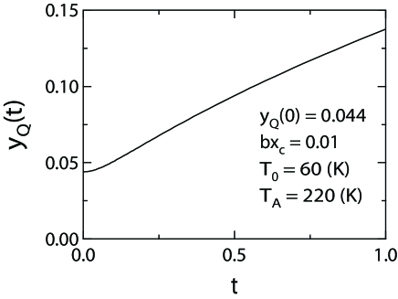
Figure 1: The solution of the basic equation of the phenomenological SCR theory for the reduced inverse static spin susceptibility $y_{Q}(t)$ as a function of the reduced temperature $t=T/T_{0}$; phenomenological parameters required to obtain $y_{Q}(t)$ in LiV₂O₄ are given in the text.

IV Calculation of $\rho(T)$ based on the SCR theory of spin fluctuations in LiV₂O₄.

First, based on the expansion (7), the resistivity $\rho(T)$ can be expressed as follows

$$\rho(T)-\rho_{imp}=\rho^{(1)}_{sf}(T)+\Delta\rho(T),$$ (16)

where the spin-fluctuation contribution $\rho_{sf}^{(1)}(T)=X_{1}^{-2}W_{1x,1x}^{sf}$ represents the lowest-order solution and $\Delta\rho(T)$ is a correction due to higher-order terms in Eq.(7). Their variations with $T$ can be found by calculating the function ${\mathcal{F}}(T)$, Eq.(15), entering the matrix elements of the spin-fluctuation scattering operator, Eq.(13). Although the subsequent derivation of an explicit form of ${\mathcal{F}}(T)$ has much in common with earlier studiesUeda77 ; Kondo02 of nearly AFM metals, essential features specific to LiV₂O₄ have to be emphasized. In particular, within the SCR theory of spin fluctuations the imaginary part of the dynamic spin susceptibility can be parametrized as followsYushankhai08

$$\mbox{Im}\chi\left({\bf Q}_{c}+{\bf q},\epsilon;T\right)=\frac{1}{4\pi T_{A}T_{0}}\frac{\epsilon}{\left[y_{Q}\left(T\right)+\left(q^{||}/q_{B}\right)^{2}+b\left({\bf q}^{\bot}/q_{B}\right)^{2}\right]^{2}+\left(\epsilon/2\pi T_{0}\right)^{2}}.$$ (17)

Here, for a given ${\bf Q}_{c}$, $q^{||}$ and ${\bf q}^{\bot}$ are the components of ${\bf q}$ parallel and perpendicular to ${\bf Q}_{c}$, respectively; $q_{B}$ is the effective radius of the BZ boundary given in terms of a primitive cell volume $v_{0}$ as $q_{B}=\left(6\pi^{2}/v_{0}\right)^{1/3}$. The parameters $T_{A}\simeq$ 220K and $T_{0}\simeq$ 60K characterize the widths of the momentum and energy distributions of spin fluctuations, respectively; a small parameter $b$ takes care about a strong anisotropy of the distribution in ${\bf k}$ space. Next, the reduced inverse susceptibility at ${\bf Q}_{c}$ is defined as $y_{Q}\left(T\right)=[2T_{A}\chi\left(Q_{c};T\right)]^{-1}$ assuming a ”spherical” approximation, i.e. $\chi\left({\bf Q}_{c};T\right)$ does not depend on a direction of ${\bf Q}_{c}$.

With the insertion of Eq.(17) into Eq.(15), we get

$${\mathcal{F}}(T)=\frac{2\pi T_{0}}{T_{A}}\int\frac{d^{3}q}{(2\pi)^{3}}\int\limits_{0}^{\infty}d\lambda n(\lambda)[n(\lambda)+1]\frac{\lambda^{2}}{\lambda^{2}+(2\pi u_{\bf q})^{2}}=\frac{2\pi T_{0}}{T_{A}}\int\frac{d^{3}q}{(2\pi)^{3}}I(u_{\bf q}).$$ (18)

Here, the last equality defines $I(u_{\bf q})$, where

$$u_{\bf q}(t)=\frac{y_{Q}\left(t\right)+\left(q^{||}/q_{B}\right)^{2}+b\left({\bf q}^{\bot}/q_{B}\right)^{2}}{t},$$ (19)

and $t=T/T_{0}$ is the reduced temperature. At the next step, the function $I(u_{\bf q})$ can be expressed as

$$I(u_{\bf q})=\frac{u_{\bf q}}{2}\left[\psi^{\prime}(u_{\bf q})-\frac{1}{u_{\bf q}}-\frac{1}{2u_{\bf q}^{2}}\right],$$ (20)

where $\psi(u)$ is the digamma function and $\psi^{\prime}(u)=d\psi(u)/du$.

The integration over ${\bf q}$ in Eq.(18) are performed by using the same prescriptions as in Ref.Yushankhai08, , which yields $(2\pi)^{-3}\int d^{3}qI(u_{\bf q})=c{\bar{f}}(T/T_{0})$, where $c$ is the known dimensionless factor, $c\approx 4$, andKondo02

$${\bar{f}}(T/T_{0})=\frac{t}{bx_{c}} \int\limits_{0}^{z_{c}}dz\left[-\frac{bx_{c}}{t}-\frac{1}{2}\ln\left(\frac{y_{Q}(t)+z^{2}+bx_{c}}{y_{Q}(t)+z^{2}}\right)\right.+$$ (21)

$$\frac{y_{Q}(t)+z^{2}+bx_{c}}{t}\psi\left(\frac{y_{Q}(t)+z^{2}+bx_{c}}{t}\right)-\frac{y_{Q}(t)+z^{2}}{t}\psi\left(\frac{y_{Q}(t)+z^{2}}{t}\right)-$$

$$\left.\ln\Gamma\left(\frac{y_{Q}(t)+z^{2}+bx_{c}}{t}\right)+\ln\Gamma\left(\frac{y_{Q}(t)+z^{2}}{t}\right)\right],$$

where $\Gamma(u)$ is the gamma function, the cutoff $z_{c}\simeq$1/2 and the remaining parameter $bx_{c}\simeq 10^{-2}$.

For a given $y_{Q}(t)$, the expression (21), as a function of temperature, can be calculated numerically. This determines, according to Eqs.(13),(18)-(21), an evolution with $T$ of any non-vanishing matrix element $W_{LL^{\prime}}^{sf}$ in the whole range $T<$ 40K, where the SCR theory for the AFM spin fluctuations in LiV₂O₄ is proved to be validYushankhai08 . Here we utilize the known functional form for $y_{Q}(t)$, Fig.1, obtained by solving the basic equation of the SCR theory developed in Ref.Yushankhai08, to explain results of inelastic neutron scattering measurements on LiV₂O₄. The solution shows that $y_{Q}(t)$ is a monotonically increasing function of temperature; the limiting value $y_{Q}(t\to 0)$, was found to be $y_{Q}(0)=$0.044. The use of the energy scale, $T^{\ast}=2\pi T_{0}y_{Q}(0)\approx$ 16K, which is the relaxation rate of the low-energy spin fluctuations,Yushankhai08 is helpful in recognizing two regimes with different power-law behavior of $y_{Q}(t)$. Actually, for $T\ll T^{\ast}$, one obtains $[y_{Q}(t)-y_{Q}(0)]/y_{Q}(0)\ll 1$, which leads to the quadratic behavior of ${\bar{f}}(T/T_{0})\sim T^{2}$. For $T^{\ast}<T$, a smooth, nearly linear, $t$-dependence of $y_{Q}(t)$ results in a peculiar monotonic temperature increase of ${\bar{f}}(T/T_{0})$, as indicated below.

First, we analyze the lowest-order approximation to the low temperature ($T\ll T^{\ast}$) resistivity,

$$\rho(T)\approx\rho_{imp}+\rho^{(1)}_{sf}(T),$$ (22)

where

$$\rho^{(1)}_{sf}(T)={\mathcal{A}}^{(1)}_{sf}{\bar{f}}(T/T_{0}),$$ (23)

and compare its $T$-dependence with that of the observedTakagi99 experimental resistivity. Here ${\mathcal{A}}^{(1)}_{sf}=(2\pi cT_{0}/T_{A})X_{1}^{-2}C_{1x,1x}$ is an adjustable parameter (together with $\rho_{imp}$) in a low-$T$ fit procedure using the calculated ${\bar{f}}(T/T_{0})$ shown in Fig.2.

One may see that the function ${\bar{f}}(T/T_{0})$ nearly precisely follows the quadratic dependence, ${\bar{f}}(T/T_{0})=c_{1}T^{2}$ with $c_{1}=$ 0.0033, for $T<$ 2K $\ll T^{\ast}$, where the Fermi-liquid behavior $[\rho^{exp}(T)-\rho_{imp}]=AT^{2}$ in LiV₂O₄ was reported.Takagi99 ; Urano00 From the low-$T$ fit procedure, as shown in Fig.3, the parameter ${\mathcal{A}}^{(1)}_{sf}$ was found to be ${\mathcal{A}}^{(1)}_{sf}=$ 666.7 $\mu\Omega cm$, which corresponds to the observed coefficient of the $T^{2}$ term, $A=$ 2.2 $\mu\Omega cm/K^{2}$.

With increasing $T$ and starting from $T\approx$ 2K, both the calculated $\rho^{(1)}_{sf}(T)$ and the measured resistivity $[\rho^{exp}(T)-\rho_{imp}]$ show gradual deviations from the $T^{2}$ behavior, however, with somewhat different rates. Specifically, starting from $T\approx$ 2K one obtains the growing discrepancy $[\rho^{exp}(T)-\rho_{imp}]-\rho^{(1)}_{sf}(T)=\Delta\rho(T)<$ 0, which indicate that the higher-order corrections involved in $\Delta\rho(T)$ cannot be longer neglected. Remarkably, a negative correction, $\Delta\rho(T)<0$, is consistent with the variational principle requiring that an extension of the involved basis functions should lead to an improved upper bound on $\rho(T)$.

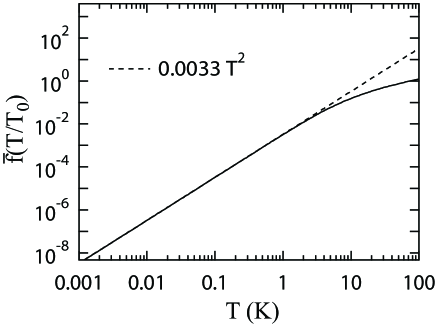
Figure 2: $T$-dependence of ${\bar{f}}(T/T_{0})$ defined by Eq.(21) and calculated with the use of the reduced inverse susceptibility $y_{Q}(T/T_{0})$ shown in Fig.1.

Actually, let us consider the lowest-order correction $\Delta\rho^{(2)}_{sf}(T)$ which can be written from Eq.(7) as

$$\Delta\rho^{(2)}_{sf}(T)=-\frac{1}{X_{1}^{2}}{\sum_{L}}^{\prime}\left[\frac{(W_{1x,L}^{sf}+W_{1x,L}^{imp})^{2}}{W_{LL}^{imp}+W_{LL}^{sf}}-\frac{(W_{1x,L}^{imp})^{2}}{W_{LL}^{imp}}\right],$$ (24)

where the second term in brackets, being already involved in $\rho_{imp}$, is now subtracted to ensure that $\Delta\rho^{(2)}_{sf}(T\to 0)=$ 0. Note that a $T$-dependence in the right-hand side of Eq.(24) is entirely due to $W_{LL^{\prime}}^{sf}=C_{LL^{\prime}}{\mathcal{F}}(T)$, both for $L^{\prime}=L$ and $L^{\prime}\not=L$. For sufficiently low $T$, a denominator in the right-hand side of Eq.(24) can be approximated assuming that $C_{LL}{\mathcal{F}}(T)\ll W_{LL}^{imp}$ and ${\mathcal{F}}(T)\sim T^{2}$, which immediately leads to small leading correction, $\Delta\rho^{(2)}_{sf}(T)\approx aT^{2}-|b|T^{4}+O(T^{6})$. Here, the first quadratic term can be adopted by changing slightly a value of the adjustable parameter ${\mathcal{A}}^{(1)}_{sf}$, while the next term, $-|b|T^{4}$, provides the required negative correction to the first-order result $\rho^{(1)}_{sf}(T)$.

An extension of the above analysis to higher temperature could be possible if one establishes reliable relations between numerous matrix elements involved in Eq.(7). The following plausible assumption can be made based on the fact that ${\mathcal{F}}(T)=(2\pi cT_{0}/T_{A}){\bar{f}}(T/T_{0}$) is a rapidly growing function of $T$, Fig.2. For instance, ${\mathcal{F}}(T\sim 30\mbox{K})$/${\mathcal{F}}(T\sim 1\mbox{K})\sim 10^{2}$. We suggest that the limit, $C_{LL}{\mathcal{F}}(T)\gg W_{LL}^{imp}$, can be achieved at $T\lesssim$ 40K, i.e near the border where the SCR theory of spin fluctuations in LiV₂O₄ is still valid. With this assumption, one obtains, for instance, the following estimate for the second order correction, $\Delta\rho^{(2)}_{sf}(T)\approx-[X_{1}^{-2}{\sum_{L}}^{\prime}(C_{1x,L})^{2}/C_{LL}]{\mathcal{F}}(T)+const$. Then, by doing in the same manner and after collecting all leading terms in the expansion (7), the physical resistivity in LiV₂O₄ for 2K$\ll T\lesssim$ 40K can be approximated by the following simple functional form

$$\rho(T)\approx\rho_{imp}+{\mathcal{B}}+{\mathcal{A}}_{sf}{\bar{f}}(T/T_{0}),$$ (25)

where

$${\mathcal{A}}_{sf}=\frac{2\pi cT_{0}}{T_{A}}\frac{1}{X_{1}^{2}}\left[C_{1x,1x}-{\sum_{L}}^{\prime}\frac{(C_{1x,L})^{2}}{C_{LL}}+{\sum_{LL^{\prime}}}^{\prime}\frac{C_{1x,L}C_{LL^{\prime}}C_{L^{\prime},1x}}{C_{LL}C_{L^{\prime}L^{\prime}}}-...\right].$$ (26)

$${\mathcal{B}}=\frac{1}{X_{1}^{2}}{\sum_{L}}^{\prime}\left\{W_{LL}^{imp}\left(\frac{C_{1x,L}}{C_{LL}}\right)^{2}+W_{1x,L}^{imp}\left[1-2\frac{C_{1x,L}}{C_{LL}}\right]-...\right\}$$ (27)

By noting a close similarity between Eq.(25) and Eq.(22), it is worth emphasizing completely different $T$-dependence of ${\bar{f}}(T/T_{0})$ in the low- and a high-temperature regimes. Moreover, the factor ${\mathcal{A}}_{sf}$ is subjected to a special constraint with respect to ${\mathcal{A}}_{sf}^{(1)}$. Actually, for $T<$ 2K $\ll T^{\ast}$ the first-order term in the series (26) is only needed, ${\mathcal{A}}_{sf}^{(1)}\simeq(2\pi cT_{0}/T_{A})X_{1}^{-2}C_{1x,1x}$, while for 2K $\ll T\lesssim$ 40K, the factor $A_{sf}$ is given by the full series (26) and, hence, ${\mathcal{A}}_{sf}<{\mathcal{A}}_{sf}^{(1)}$ is required. An estimate for a shift ${\mathcal{B}}$ in Eq.(25), which is the second adjustable parameter in a high-$T$ fit procedure, is discussed bellow.

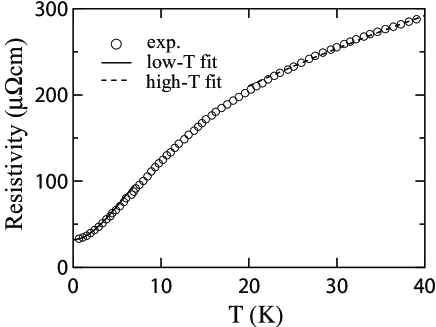
Figure 3: Theoretical fits to the experimental data (Ref.Takagi99, , open circles) for the electrical resistivity in LiV₂O₄ in different temperature regions. In the low-$T$ limit, the resistivity is described by Eqs.(22),(23) with $\rho_{imp}=32(\mu\Omega{\rm cm})$ and $A_{sf}^{(1)}=666.7(\mu\Omega{\rm cm})$. In the high temperature region, 20 K $<T<$ 40 K, where the SCR theory is still valid, the resistivity is approximated by Eq.(25) with $\rho_{imp}+{\mathcal{B}}=117(\mu\Omega{\rm cm})$ and $A_{sf}=280(\mu\Omega{\rm cm})$.

In Fig.3, the physical resistivity $[\rho^{exp}(T)-\rho_{imp}]$ is compared with the predicted behavior, Eq.(25), for $T>T^{\ast}(\approx$ 16K). A satisfactory coincidence between the experimental data and calculated results is achieved for 20K $<T<$ 40K with two fit parameters ${\mathcal{A}}_{sf}=280\mu\Omega cm$ and ${\mathcal{B}}=85\mu\Omega cm$. While the expected constraint, ${\mathcal{A}}_{sf}<{\mathcal{A}}_{sf}^{(1)}$ is fulfilled, the obtained large value of ${\mathcal{B}}\approx 3\rho_{imp}$ means that the Matthiessen ruleZiman60 is severely violated. A possible mechanism for this effect is the following. Recalling the estimate, Eq.(27) for ${\mathcal{B}}$, together with relations $\rho_{imp}\sim W_{1x,1x}^{imp}$ and $\left(C_{1x,L}/C_{LL}\right)^{2}\ll$ 1, we suggest that for some $L\not=1x$ one has $W_{LL}^{imp}\gg W_{1x,1x}^{imp}$, which explains why an estimate ${\mathcal{B}}\sim\rho_{imp}$ is feasible.

So far the special attention has been paid to two limiting regimes of low- and comparatively high-temperatures ($T<$ 40K), where the series expansion, Eq.(7), for $\rho(T)$ reduces to very similar forms, Eqs. (22) and (25), requiring two adjustable parameters for a fit procedure in each regimes . We insist that Eq.(7) should provide the interpolation $T$-dependent function between the low- and high-$T$ limits as well. However, for intermediate temperatures, one has $C_{LL}{\mathcal{F}}(T)\sim W_{LL}^{imp}$, and the corresponding fit procedure, though being possible, would require a larger number of adjustable parameters. This could hardly give more insight into the problem under consideration and therefore we omit such a procedure in our discussion.

V Conclusion

We have calculated the electrical resistivity $\rho(T)$ in the paramagnetic metallic spinel LiV₂O₄ treated as a nearly AFM Fermi-liquid for temperatures $T<$ 40K . Impurities and strongly degenerate temperature-induced low-energy AFM spin fluctuations were supposed to provide two main sources of the quasiparticle scattering and the resistivity. The self-consistent renormalization theory developed earlier was applied to derive explicitly the temperature-dependent matrix elements of the spin fluctuation scattering operator. The absence of hot spots of the Fermi surface and a largely isotropic character of the quasiparticle scattering was deduced from a peculiar, nearly spherical, shape of the spin-fluctuation distribution in the momentum space for the paramagnetic ground state in LiV₂O₄. Comparatively weak anisotropic effects were assumed to originate mainly from a complex many-sheet structure of the Fermi surface in this compound. The assumption allowed us to use the variational solution for the Boltzmann equation in the form of a perturbative series expansion for $\rho(T)$. Our theory remains to be a phenomenological one since unknown model parameters were found from the best overall fit to the temperature-dependent $\rho^{exp}(T)$ measured on a single crystal of LiV₂O₄.

The resulting theoretical expression for $\rho(T)$ was shown to take very similar simple forms in two limiting regimes for spin fluctuations, which describe successfully experimental results for $\rho(T)$ with a minimal set of two adjustable parameters in each regime. These include the low temperatures, $T\ll T^{\ast}$ (where $T^{\ast}\approx$ 16K is the characteristic energy scale of spin fluctuations), and somewhat higher temperatures, $T^{\ast}<T<$ 40K, respectively.

For $T>$ 40K the SCR theory of AFM spin fluctuations in LiV₂O₄ is no longer valid. As discussed in Ref.Yushankhai08, , and evidenced from experimentTakagi99 ; Urano00 ; Krimmel99 ; Lee01 ; Murani04 , with increasing $T$ the AFM fluctuations at $|{\bf q}|\simeq Q_{c}$ are suppressed and no more distinguished from those at other wave vectors in the BZ; the system enters a spin localized regime compatible with the Curie-Weiss behavior of $\chi({\bf q}=0)$ observed in LiV₂O₄ for $T>50$ K. An explanation of incoherent transport properties in this regime remains to be a challenging problem.

VI Acknowledgments

One of the authors (V.Yu.) acknowledges partial financial support from the Heisenberg-Landau program.

References

- (1) S. Kondo, D.C. Johnston, C.A. Swenson et al., Phys. Rev. Lett. 78, 3729 (1997)
- (2) D. C. Johnston, Physica B (Amsterdam) 281-282, 21 (2000)
- (3) S. Kondo, D.C. Johnston, and L.L. Miller, Phys. Rev. B 59, 2609 (1999)
- (4) V. Yushankhai , A. Yaresko, P. Fulde and P. Thalmeier, Phys. Rev. B 76, 085111 (2007)
- (5) A. Krimmel, A. Loidl, M. Klemm, and S. Horn, and H. Schober, Phys. Rev. Lett. 82, 2919 (1999)
- (6) S.-H. Lee, Y. Qiu, C. Broholm, Y. Ueda, and J.J. Rush, Phys. Rev. Lett. 86, 5554 (2001)
- (7) A.P. Murani, A. Krimmel, J.R. Stewart, M. Smith, P. Strobel, A. Loidl and A. Ibarra-Palos, J. Phys: Condensed Matter 16, p.S607 (2004)
- (8) V. Yushankhai, P. Thalmeier, and T. Takimoto, Phys. Rev. B 77, 125126 (2008)
- (9) V. Yushankhai, T. Takimoto, and P. Thalmeier, J. Phys: Condensed Matter 20, 465221 (2008)
- (10) H. Takagi, C. Urano, S. Kondo, M. Nohara, Y. Ueda, T. Shiraki, T. Okubo, Materials Science and Engineering, B 63, 147 (1999)
- (11) C. Urano, M. Nohara, S. Kondo, F. Sakai, H. Takagi, T. Shiraki, and T. Okubo, Phys. Rev. Lett. 85, 1052 (2000)
- (12) P.E. Jönsson, K. Takenaka, S. Niitaka, T. Sasagawa, S. Sugai, and H. Takagi, Phys. Rev. Lett. 99, 167402 (2007)
- (13) A. Irizawa, K. Shimai, T. Nanba, S. Niitaka and H. Takagi, J. Phys: Conference Series 200, 012068 (2010)
- (14) V. Yushankhai , P. Fulde and P. Thalmeier, Phys. Rev. B 71, 245108 (2005)
- (15) R. Hlubina and T.M. Rice, Phys. Rev. B 51, 9253 (1995)
- (16) A. Rosch, Phys. Rev. Lett. 82, 4280 (1999)
- (17) A. Rosch, Phys. Rev. B 62, 4945 (2000)
- (18) T. Moriya, Spin Fluctuations in Itinerant Electron Magnetism, Springer Ser. Solid-State Science Vol. 56, (Springer, Berlin, 1985)
- (19) T. Moriya and A. Kawabata, J. Phys. Soc. Jpn. 34, 639 (1973)
- (20) H. Hasegawa and T. Moriya, J. Phys. Soc. Jpn. 36, 1542 (1974)
- (21) K. Fujiwara, K. Miyoshi, J. Takeuchi, Y. Shimaoka and T. Kobayashi, J. Phys: Condensed Matter 16, p.S615 (2004)
- (22) K. Ueda and T. Moriya, J. Phys. Soc. Jpn. 39, 605 (1975)
- (23) K. Ueda, J. Phys. Soc. Jpn. 43, 1497 (1977)
- (24) J. Ziman, Electrons and Phonons (Clarendon, Oxford, 1960)
- (25) P. Allen, Phys. Rev. B 13, 1416 (1976)
- (26) P. Allen, Phys. Rev. B 17, 3725 (1978)
- (27) H. Kondo, J. Phys. Soc. Jpn. 71, 3011 (2002)