Optimization over Geodesics for Exact Principal Geodesic Analysis

Abstract

In fields ranging from computer vision to signal processing and statistics, increasing computational power allows a move from classical linear models to models that incorporate non-linear phenomena. This shift has created interest in computational aspects of differential geometry, and solving optimization problems that incorporate non-linear geometry constitutes an important computational task. In this paper, we develop methods for numerically solving optimization problems over spaces of geodesics using numerical integration of Jacobi fields and second order derivatives of geodesic families. As an important application of this optimization strategy, we compute exact Principal Geodesic Analysis (PGA), a non-linear version of the PCA dimensionality reduction procedure. By applying the exact PGA algorithm to synthetic data, we exemplify the differences between the linearized and exact algorithms caused by the non-linear geometry. In addition, we use the numerically integrated Jacobi fields to determine sectional curvatures and provide upper bounds for injectivity radii.

1 Introduction

Manifolds, sets locally modeled by Euclidean spaces, have a long and intriguing history in mathematics, and topological, differential geometric, and Riemannian geometric properties of manifolds have been studied extensively. The introduction of high performance computing in applied fields has widened the use of differential geometry, and Riemannian manifolds, in particular, are now used for modeling a range of problems possessing non-linear structure. Applications include shape modeling (complex projective shape spaces kendall_shape_1984 and medial representations of surfaces blum_transformation_1967 ; joshi_multiscale_2002 ), imaging (tensor manifolds in diffusion tensor imaging fletcher_principal_2004 ; fletcher_riemannian_2007 ; pennec_riemannian_2006 and image segmentation and registration caselles_geodesic_1995 ; pennec_feature-based_1998 ), and several other fields (forestry huckemann_intrinsic_2010 , human motion modeling sminchisescu_generative_2004 ; urtasun_priors_2005 , information geometry and signal processing yang_means_2011 ).

To fully utilize the power of manifolds in applied modeling, it is essential to develop fast and robust algorithms for performing computations on manifolds, and, in particular, availability of methods for solving optimization problems is paramount. In this paper, we develop methods for numerically solving optimization problems over spaces of geodesics using numerical integration of Jacobi fields and second order derivatives of geodesic families. In addition, the approach allows numerical approximation of sectional curvatures and bounds on injectivity radii huckemann_intrinsic_2010 . The methods apply to manifolds represented both parametrically and implicitly without preconditions such as knowledge of explicit formulas for geodesics. This fact makes the approach applicable to a range of applications, and it allows exploration of the effect of curvature on non-linear statistical methods.

To exemplify this, we consider the problem of capturing the variation of a set of manifold valued data with the Principal Geodesic Analysis (PGA, fletcher_principal_2004-1 ) non-linear generalization of Principal Component Analysis (PCA). Until now, there has been no method for numerically computing PGA for general manifolds without linearizing the problem. Because PGA can be formulated as an optimization problem over geodesics, the tools developed here apply to computing it without discarding the non-linear structure. As a result, the paper provides an algorithm for computing exact PGA for a wide range of manifolds.

1.1 Related Work

A vast body of mathematical literature describes manifolds and Riemannian structures; do_carmo_riemannian_1992 ; lee_riemannian_1997 provide excellent introductions to the field. From an applied point of view, the papers dedieu_symplectic_2005 ; herbert_bishop_keller_numerical_1968 ; noakes_global_1998 ; klassen_geodesics_2006 ; schmidt_shape_2006 ; sommer_bicycle_2009 address first-order problems such as computing geodesics and solving the exponential map inverse problem, the logarithm map. Certain second-order problems including computing Jacobi fields on diffeomorphism groups younes_evolutions_2009 ; ferreira_newton_2008 have been considered but mainly on limited classes of manifolds. Different aspects of numerical computation on implicitly defined manifolds are covered in zhang_curvature_2007 ; rheinboldt_manpak:_1996 ; rabier_computational_1990 , and generalizing linear statistics to manifolds has been the focus of the papers karcher_riemannian_1977 ; pennec_intrinsic_2006 ; fletcher_robust_2008 ; fletcher_principal_2004-1 ; huckemann_intrinsic_2010 .

Optimization problems can be posed on a manifold in the sense that the domain of the cost function is restricted to the manifold. Such problems are extensively covered in the literature (e.g. luenberger_gradient_1972 ; yang_globally_2007 ). In contrast, this paper concerns optimization problems over geodesics with the complexity residing in the cost functions and not the optimization domains.

The manifold generalization of linear PCA, PGA, was first introduced in fletcher_statistics_2003 but it was formulated in the form most widely used in fletcher_principal_2004-1 . It has subsequently been used for several applications. To mention a few, the authors in fletcher_principal_2004-1 ; fletcher_principal_2004 study variations of medial atoms, wu_weighted_2008 uses a variation of PGA for facial classification, said_exact_2007 presents examples on motion capture data, and sommer_bicycle_2009 applies PGA to vertebrae outlines. The algorithm presented in fletcher_principal_2004-1 for computing PGA with tangent space linearization is most widely used. In contrast, said_exact_2007 computes PGA as defined in fletcher_statistics_2003 without approximations, exact PGA, on a particular manifold, the Lie group $\mathrm{SO}(3)$. The paper sommer_manifold_2010 uses the methods presented here to experimentally assess the effect of tangent space linearization on high dimensional manifolds modeling real-life data.

A recent wave of interest in manifold valued statistics has lead to the development of Geodesic PCA (GPCA, huckemann_intrinsic_2010 ) and Horizontal Component Analysis (HCA, sommer_horizontal_2013 ). GPCA is in many respects close to PGA but GPCA optimizes for the placement of the center point and minimizes projection residuals along geodesics. HCA builds low-dimensional orthogonal decompositions in the frame bundle of the manifold that project back to approximating subspaces in the manifold.

1.2 Content and Outline

The paper presents two main contributions: (1) how numerical integration of Jacobi fields and second order derivatives can be used to solve optimization problems over geodesics; and (2) how the approach allows numerical computation of exact PGA. In addition, we use the computed Jacobi fields to numerically approximate geometric properties such as sectional curvatures. After a brief discussion of the geometric background, explicit differential equations for computing Jacobi fields and second derivatives of geodesic families are presented in Section 3. The actual derivations are performed in the appendices due to their notational complexity. In Section 4, the exact PGA algorithm is developed. We end the paper with experiments that illustrate the effect of curvature on the non-linear statistical method and with estimation of sectional curvatures and injectivity radii bounds.

The importance of curvature computations is noted in huckemann_intrinsic_2010 , which lists the ability to compute sectional curvature as a high importance open problem. The paper presents a partial solution to this problem: we discuss how sectional curvatures can be determined numerically when either a parametrization or implicit representation is available.

In the experiments, we evaluate how the differences between the exact and linearized PGA depend on the curvature of the manifold. This experiment, which to the best of our knowledge has not been made before, is made possible by the generality of the optimization approach that makes the algorithm applicable to a wide range of manifolds with varying curvature.

2 Background

This section will include brief discussions of relevant aspects of differential and Riemannian geometry. We keep the notation close to the notation used in the book do_carmo_riemannian_1992 ; see in addition Appendix A.

2.1 Manifolds and Their Representations

In the sequel, $M$ will denote a Riemannian manifold of finite dimension $\eta$. We will need $M$ to be sufficiently smooth, i.e. of class $C^{k}$ for $k=3$ or $4$ depending on the application. For concrete computational applications, we will represent $M$ either using parametrizations or implicitly. A local parametrization is a map $\mathbf{x}\in C^{k}(U,M)$ from an open subset $U\subset\mathbb{R}^{\eta}$ to $M$. With an implicit representation, $M$ is represented as a level set of a differentiable map $F:\mathbb{R}^{m}\rightarrow\mathbb{R}^{n}$, e.g. $M=F^{-1}(0)$. If the Jacobian matrix $DF$ has full rank $n$ everywhere on $M$, $M$ will be an $(m-n)$-dimensional manifold. The space $\mathbb{R}^{m}$ is called the embedding space. When dealing with implicitly defined manifolds, we let $m$ and $n$ denote the dimension of the domain and codomain of $F$, respectively, so that the dimension $\eta$ of the manifold equals $m-n$. Examples of applications using implicit representations include shape and human poses models sommer_bicycle_2009 ; hauberg_natural_2012 , and several shape models use parametric representations joshi_multiscale_2002 ; klassen_analysis_2004 .

2.2 Geodesic Systems

Given a local parametrization $\mathbf{x}:U\rightarrow M$, a curve $\alpha_{t}$ on $M$ is a geodesic if the curve $x_{t}$ in $U$ representing $\alpha_{t}$, i.e. $\mathbf{x}^{-1}\circ\alpha_{t}=x_{t}$, satisfies the ODE

$$\ddot{x}_{t}^{k}=-\sum_{i,j}^{\eta}\Gamma_{ij}^{k}(x_{t})\dot{x_{t}}^{i}\dot{x_{t}}^{j},\ k=1,\ldots,\eta\ .$$ (1)

Here $\Gamma_{ij}^{k}$ denotes the Christoffel symbols of the Riemannian metric. Conversely, geodesics can be found by solving the ODE with a starting point $x_{0}=q$ and initial velocity $\dot{x}_{0}=v$ as initial conditions. The exponential map $\mathrm{Exp}_{q}v$ maps the initial point $q\in M$ and velocity $v\in T_{q}M$ to $\alpha_{1}$, the point on the geodesic at time $t=1$. When defined, the logarithm map $\mathrm{Log}_{q}y$ is the inverse of $\mathrm{Exp}_{q}$, i.e. $\mathrm{Exp}_{q}\mathrm{Log}_{q}y=y$. For implicitly represented manifolds, the classical ODE describing geodesics is not directly usable because neither parametrizations nor Christoffel symbols are directly available. Instead, the geodesic with initial point $q$ and initial velocity $v$ can be found as the $x$-part of the solution of the IVP

$$\begin{split}&\dot{p}_{t}=-\left(\sum_{k=1}^{n}\mu^{k}(x_{t},p_{t})H_{x_{t}}(F^{k})\right)\dot{x}_{t}\ ,\\ &\dot{x}_{t}=\left(I-D_{x_{t}}F^{\dagger}D_{x_{t}}F\right)p_{t}\ ,\\ &x_{0}=q,\ p_{0}=v\ ,\end{split}$$ (2)

see dedieu_symplectic_2005 . Note that $x_{t}$ is a curve in the embedding space $\mathbb{R}^{m}$ but since $M$ is a subset of the embedding space and the starting point $q$ is in $M$, $x_{t}$ will stay in $M$ for all $t$. Recall that $F:\mathbb{R}^{m}\rightarrow\mathbb{R}^{n}$ is the map defining the manifold by e.g. $M=F^{-1}(0)$ and that $H(F^{k})$ denotes the Hessian of the $k$th component of $F$. $F$ is map between Euclidean spaces and the Hessian is therefore the ordinary Euclidean Hessian matrix. The map $\mu:\mathbb{R}^{m}\times\mathbb{R}^{m}\rightarrow\mathbb{R}^{n}$ is defined by $(x,p)\mapsto-(D_{x}F^{T})^{\dagger}p$ where the symbol $DF^{\dagger}$ denotes the generalized inverse or pseudo-inverse of the non-square matrix $DF$. Since $DF$ has full-rank $n$, $DF^{\dagger}$ equals $DF^{T}(DFDF^{T})^{-1}$. Numerical stability of the geodesic system is treated in dedieu_symplectic_2005 .

2.3 Geodesic Families and Variations of Geodesics

In the next sections, we will treat optimization problems over geodesics of which the PGA problem (6) constitute a concrete example; in addition, problems such as geodesic regression fletcher_geodesic_2011 and manifold total least squares belong to this class. For this purpose, we here recall the close connection between variations of geodesics, Jacobi fields, and the differential $d\mathrm{Exp}$. Let $\alpha_{t,s}$ be a family of geodesics parametrized by $s$, i.e. for each $\tilde{s}$, the curve $t\mapsto\alpha_{t,\tilde{s}}$ is a geodesic. By varying the parameter $s$, a vector field $\tfrac{d}{ds}\alpha_{t,0}$ is obtained. These Jacobi fields are uniquely determined by the initial conditions $J_{0}$ and $\tfrac{D}{dt}J_{0}$, the variation of the initial points $x_{0,s}$ and the covariant derivative of the field at $t=0$, respectively. Define $q_{s}=x_{0,s}$, $v_{s}=\dot{x}_{0,s}$, and $w=\tfrac{d}{ds}v_{0}$. If $\tfrac{d}{ds}q_{0}=J_{0}$ and $w=\tfrac{D}{dt}J_{0}$ then $\tfrac{d}{ds}\mathrm{Exp}_{q_{s}}(tv_{s})|_{s=0}$ equals $J_{t}$ (do_carmo_riemannian_1992, , Chap. 5). When $q_{s}$ is constant, i.e. $q_{s}=q$, we have the following connection between $J_{t}$ and the differential $d\mathrm{Exp}$:

$$d_{tv_{0}}\mathrm{Exp}_{q}tw=J_{t}\ .$$ (3)

Jacobi fields can equivalently be defined as solutions to an ODE that involves the curvature endomorphism of the manifold (do_carmo_riemannian_1992, , Chap. 5). However, the curvature endomorphism is not easily computed when the manifold is represented implicitly, and, therefore, the ODE is hard to use for computational applications in this case. In the next section, we numerically compute Jacobi fields by integrating the differential of the system (2).

Figure 1: The sphere $\mathbb{S}^{2}$ with a Jacobi field along a geodesic connecting the poles. Each pole is a conjugate point to the other since the non-zero Jacobi field vanishes. The injectivity radius is equal to the length of the geodesic, $\pi$.

Jacobi fields can be used to retrieve various geometric information e.g. sectional curvature. Let $J_{t}$ denote a Jacobi field along the geodesic $\alpha_{t}$ with $J_{0}=0$ and derivative $w=\tfrac{D}{dt}J_{0}$. Assume the vectors $v_{0}=\dot{\alpha}_{0}$ and $w$ are orthonormal. These vectors define a plane $\sigma=\mathrm{span}\,\{v_{0},w\}$ in $T_{\alpha_{0}}M$, and $K_{\alpha_{0}}(\sigma)$ denotes the sectional curvature of the plane $\sigma$. Because $K_{\alpha_{0}}(\sigma)$ occurs in a Taylor expansion of the length $\|J_{t}\|$, the sectional curvature can be estimated by

$$K_{\alpha_{0}}(\sigma)\approx\frac{6}{t^{3}}(t-\|J(t)\|)$$ (4)

for small $t$. Furthermore, if $J_{t}$ is a non-zero Jacobi field with $J_{0}=0$ along a geodesic $\alpha_{t}$ and, for some $\tilde{t}>0$, also $J_{\tilde{t}}=0$ then $\alpha_{\tilde{t}}$ is called a conjugate point to $\alpha_{0}$. This can provide an upper bound on the injectivity radius of $M$, that, in general terms, specifies the minimum length of non-minimizing geodesics. Figure 1 illustrates the situation on the sphere $\mathbb{S}^{2}$. We will explore both these points in the experiments section.

2.4 Principal Geodesic Analysis

Principal Component Analysis (PCA) is widely used to model the variability of data in Euclidean spaces. The procedure provides linear dimensionality reduction by defining a sequence of linear subspaces maximizing the variance of the projection of the data to the subspaces or, equivalently, minimizing the reconstruction errors. The $k$th subspace is spanned by an orthogonal basis $\{v^{1},\ldots,v^{k}\}$ of principal components $v^{1},\ldots,v^{k}$, and the $i$th principal component is defined recursively by

$$v^{i}=\mathrm{argmax}_{\|v\|=1}\frac{1}{N}\sum_{j=1}^{N}\left(\left<x_{j},v\right>^{2}+\sum_{l=1}^{i-1}\left<x_{j},v^{l}\right>^{2}\right)$$ (5)

when formulated as to maximize the variance of the projection of the dataset $\{x_{1},\ldots,x_{N}\}$ to the subspaces $\mathrm{span}\,\{v^{1},\ldots,v^{i-1}\}$.

PCA is dependent on the vector space structure of the Euclidean space and hence cannot be performed on manifold valued datasets. Principal Geodesic Analysis was developed to overcome this limitation. PGA finds geodesic subspaces centered at point $\mu\in M$ with $\mu$ usually being an intrinsic mean of the dataset $\{x_{1},\ldots,x_{N}\}$, $x_{j}\in M$. The $k$th geodesic subspace $S_{k}$ of $T_{\mu}M$ is defined as $\mathrm{Exp}_{\mu}(V_{k})$ with $V_{k}=\mathrm{span}\,\{v^{1},\ldots,v^{k}\}$ being the span of the principal directions $v^{1},\ldots,v^{k}$ defined recursively by

$$\begin{split}&v^{i}=\mathrm{argmax}_{\|v\|=1,v\in V_{i-1}^{\perp}}\frac{1}{N}\sum_{j=1}^{N}d(\mu,\pi_{S_{v}}(x_{j}))^{2}\ ,\\ &S_{v}=\mathrm{Exp}_{\mu}(\mathrm{span}\,\{V_{i-1},v\})\ .\end{split}$$ (6)

The projection $\pi_{S}(x)$ of a point $x\in M$ onto a geodesic subspace $S=\mathrm{Exp}_{q}V$ is

$$\begin{split}\pi_{S}(x)&=\mathrm{argmin}_{y\in S}d(x,y)^{2}=\mathrm{argmin}_{y\in S}\|\mathrm{Log}_{y}x\|^{2}\\ &=\mathrm{Exp}_{q}(\mathrm{argmin}_{w\in V}\|\mathrm{Log}_{\mathrm{Exp}_{q}w}x\|^{2})\ .\end{split}$$ (7)

The term being maximized in (6) is the sample variance of the projected data, the expected value of the squared distance to $\mu$, and PGA therefore extends PCA by finding geodesic subspaces in which variance is maximized.

Since both optimization problems (6) and (7) are difficult to optimize, PGA has traditionally been computed using the orthogonal projection in the tangent space of $\mu$ to approximate the true projection. With this approximation, equation (6) simplifies to

$$v^{i}\approx\mathrm{argmax}_{\|v\|=1}\frac{1}{N}\sum_{j=1}^{N}\left(\left<\mathrm{Log}_{\mu}x_{j},v\right>^{2}+\sum_{l=1}^{i-1}\left<\mathrm{Log}_{\mu}x_{j},v^{l}\right>^{2}\right)$$

which is equivalent to (5), and, therefore, the procedure amounts to performing regular PCA on the vectors $\mathrm{Log}_{\mu}x_{j}$. We will refer to PGA with the approximation as linearized PGA, and, following said_exact_2007 , PGA as defined by (6) will be referred to as exact PGA. The ability to iteratively solve optimization problems over geodesics that we will develop in the next sections will allow us to optimize (6) and hence numerically compute exact PGA.

In general, PGA might not be well-defined as the intrinsic mean might not be unique and both existence and uniqueness may fail for the projections (7) and the optimization problem (6). The convexity bounds of Karcher karcher_riemannian_1977 ensures uniqueness of the mean for sufficiently local data but setting up sufficient conditions to ensure well-posedness of (7) and (6) for general manifolds is difficult because they depend on the global geometry of the manifold.

There is ongoing discussion of when principal components should be constrained to pass the intrinsic mean as in PGA or if other types of means should be used, see huckemann_intrinsic_2010 with discussions. In Geodesic PCA huckemann_intrinsic_2010 , the principal geodesics do not necessarily pass the intrinsic mean, and similar optimization that allows the PGA base point to move away from the intrinsic mean can be carried out with the optimization approach used in this paper. PGA can also be modified by replacing maximization of sample variance by minimization of reconstruction error. This alternate definition is not equivalent to the definition above, a fact that again underlines the difference between the Euclidean and the curved situation. We will illustrate differences between the formulations in the experiments section but we mainly use the variance formulation (6).

3 Optimization over Geodesics

Equation (6) and (7) defining PGA are examples of optimization problems over geodesics that in those cases are represented by their starting point $\mu$ and initial velocity $v$. More generally, we here consider problems

$$\min_{(q,v)\in(M,T_{q}M)}F(\mathrm{Exp}_{q}v)$$ (8)

where $F:M\rightarrow\mathbb{R}$ is a function defining the cost of the geodesic $\mathrm{Exp}_{q}tv$ here at time $t=1$.. In order to iteratively solve optimization problems of the form (8), we will need derivatives of $\mathrm{Exp}_{q}v$ since $dF(\mathrm{Exp}_{q}v)=d_{y}F\,d\mathrm{Exp}_{q}v$ with $y=\mathrm{Exp}_{q}v$. Thus, we wish to compute the differential of $\mathrm{Exp}_{q}v$ with respect to initial point $q$ and initial velocity $v$. Since (6) is a function of the projection $\pi_{S}$ given by (7), we will later see that we need the second order differential of $\mathrm{Exp}$ as well.

Only in specific cases where explicit expressions for geodesics are available can the above mention differentials be derived in closed form. Instead, for general manifolds, the ODEs (1) and (2) describing geodesics can be differentiated giving systems that can be numerically integrated to provide the differentials. This approach relies on the fact that sufficiently smooth initial value problems (IVPs) are differentiable with respect to their initial values, see e.g. (hairer_solving_2008, , Chap. I.14).

We will here derive explicit expressions for IVPs describing the differential of the exponential map and Jacobi fields. In addition, we will differentiate the IVPs a second time. The concrete expressions will allow the IVPs to be used for iterative optimization of problems on the form (8). In particular, they will be used for the exact PGA algorithm presented in the next section. The basic strategy is simple: we differentiate the geodesic systems of Section 2.2. Though the resulting equations are notationally complex, their derivation is in principle just repeated application of the chain and product rules for differentiation. MATLAB code for numerical integration of the systems is available at http://image.diku.dk/sommer.

Since the geodesic equations (2) contain the generalized inverse of the Jacobian matrix $DF$, we will use the following formula for derivatives of generalized inverses. When an $n\times m$ matrix $A_{s}$ depends on a parameter $s$ and has full rank $n$, and if its generalized inverse $A_{s}^{\dagger}$ is differentiable, then the derivative $\tfrac{d}{ds}(A_{s}^{\dagger})$ is given by

$$\tfrac{d}{ds}(A_{s}^{\dagger})=-A_{s}^{\dagger}\big{(}\tfrac{d}{ds}A_{s}\big{)}A_{s}^{\dagger}+\big{(}I-A_{s}^{\dagger}A_{s}\big{)}\big{(}\tfrac{d}{ds}A_{s}^{T}\big{)}\big{(}A_{s}^{\dagger}\big{)}^{T}A_{s}^{\dagger}A_{s}\ .$$ (9)

This result was derived in decell_derivative_1974 ; golub_differentiation_1973 and hanson_extensions_1969 for the full-rank case. We will apply (9) with $A_{s}=D_{x_{t,s}}F$ when $x_{t,s}$ is an $s$ dependent family of curves in the embedding space $\mathbb{R}^{m}$ that are geodesics on $M$ and when $t$ is fixed. To see that $D_{x_{t,s}}F^{\dagger}$ is differentiable with respect to $s$ when $x_{t,s}$ depends smoothly on $s$, take a frame of the normal space to $M$ in a neighborhood of $x_{t,s}$, and note that $D_{x_{t,s}}F^{\dagger}$ is a composition of a invertible map onto the frame depending smoothly on $s$ and the frame itself.

The explicit expressions for the differential equations are notationally heavy. Therefore, we only state the results here and postpone the actual derivation to Appendix B.
Let $M\subset\mathbb{R}^{m}$ be defined as a regular zero level set of a $C^{3}$ map $F:\mathbb{R}^{m}\rightarrow\mathbb{R}^{n}$. Using the embedding, we identify curves in $M$ and vectors in $TM$ with curves and vectors in $\mathbb{R}^{m}$. Let $x_{t}$ be a geodesic with $x_{0}=q$ and $\dot{x}_{0}=v$. The Jacobi field $J_{t}$ along $x_{t}$ with $J_{0}=u$ and $\tfrac{D}{dt}J_{0}=w$ can then be found as the $z$-part of the solution of the IVP

$$\begin{split}&\begin{pmatrix}\dot{y}_{t}\\ \dot{z}_{t}\end{pmatrix}=F_{q,v}^{I}\left(t,\begin{pmatrix}y_{t}\\ z_{t}\end{pmatrix}\right)\ ,\\ &\begin{pmatrix}y_{0}\\ z_{0}\\ \end{pmatrix}=\begin{pmatrix}w\\ u\end{pmatrix}\ ,\end{split}$$ (10)

with $F_{q,v}^{I}$ the map given in explicit form in Appendix B.
As previously noted, Jacobi fields can be described using an ODE incorporating the curvature endomorphism in the parameterized case. We can, however, apply a procedure similar to the implicit case and derive and IVP by differentiating the geodesic system (1). We will use the resulting IVP (24) when working with variations of geodesics in the parameterized case, see Appendix B.

The systems (10) and (24) are both linear in the initial values $(w\ u)^{T}$ as expected of systems describing differentials. They are non-autonomous due to the dependence on the position on the curve $x_{t}$.

Recall the equivalence (3) between Jacobi fields and $d\mathrm{Exp}$: if $(y_{t},z_{t})$ satisfy (10) (or (24)) with initial values $(w,0)^{T}$ then $d_{v}\mathrm{Exp}_{q}w$ is equal to $z_{1}$. Therefore, we can compute the differential $d_{v}\mathrm{Exp}_{q}$ with respect to $v$ by numerically integrating the system using a basis $\{w^{1},\ldots,w^{\eta}\}$ for the tangent space $T_{q}M$ at $q\in M$. With initial conditions $(0,u)^{T}$ instead, we can similarly compute the derivative with respect to the initial point $q$. Note that $\mathrm{Exp}_{q}\mathrm{Log}_{q}y=y$ implies that $d_{y}\mathrm{Log}_{q}=(d_{\mathrm{Log}_{q}y}\mathrm{Exp}_{q})^{-1}$, a fact that allows the computation of $d_{y}\mathrm{Log}_{q}$ as well.

Assuming the manifold is sufficiently smooth, we can differentiate the systems (10) and (24) once more and thereby obtain second order information that we will need later. The main difficulty is performing the algebra of the already complicated expressions for the systems, and, for the implicit case, we will need second order derivatives of the generalized inverses $D_{x_{t,s}}F^{\dagger}$. For simplicity, we consider a families of geodesics with stationary initial point. The derivations are again postponed to Appendix B.
Let $M$ be of class $C^{4}$, and let $\alpha_{t,s}$ be a family of geodesics. Assume $\mathbf{x}:U\rightarrow M$ is a local parametrization containing $\alpha_{t,s}$, and let $x_{t,s}$ be the curve in $U$ representing $\alpha_{t,s}$, i.e. $\mathbf{x}^{-1}\circ\alpha_{t,s}=x_{t,s}$. Let $w\in T_{q}M$ with $\alpha_{0,s}=q$ and $v_{s}=\dot{\alpha}_{0,s}$. Define $u=\tfrac{d}{ds}v_{0}$, and let $V_{q,v_{0},w,u}=\tfrac{d}{ds}\left(d_{v_{s}}\mathrm{Exp}_{q}w\right)=\tfrac{d}{ds}\Big{(}\tfrac{d}{dr}\left(\mathrm{Exp}_{q}v_{s}+rw\right)\Big{)}$. Then, in coordinates defined by $\mathbf{x}$, $V_{q,v_{0},w,u}$ can be found as the $r$-part of the solution of the IVP

$$\begin{split}&\begin{pmatrix}\dot{q}_{t}\\ \dot{r}_{t}\end{pmatrix}=G_{q,v_{0},w,u}^{P}\left(t,\begin{pmatrix}q_{t}\\ r_{t}\end{pmatrix}\right)\ ,\\ &\begin{pmatrix}q_{0}\\ r_{0}\\ \end{pmatrix}=\begin{pmatrix}0\\ 0\end{pmatrix}\ ,\end{split}$$ (11)

with $G_{q,v_{0},w,u}^{P}$ the map given in explicit form in Appendix B.

Now, let instead $M\subset\mathbb{R}^{m}$ be defined as a regular zero level set of a $C^{4}$ map $F:\mathbb{R}^{m}\rightarrow\mathbb{R}^{n}$. Then $V_{q,v_{0},w,u}$ can be found as the $r$-part of the solution of the IVP

$$\begin{split}&\begin{pmatrix}\dot{q}_{t}\\ \dot{r}_{t}\end{pmatrix}=G_{q,v_{0},w,u}^{I}\left(t,\begin{pmatrix}q_{t}\\ r_{t}\end{pmatrix}\right)\ ,\\ &\begin{pmatrix}q_{0}\\ r_{0}\\ \end{pmatrix}=\begin{pmatrix}0\\ 0\end{pmatrix}\ ,\end{split}$$ (12)

with $G_{q,v_{0},w,u}^{I}$ the map given in explicit form in Appendix B.
We note that solutions to (11) and (12) depend linearly on $u$ even though the systems themselves are not linear.

3.1 Numerical Considerations

The geodesic systems (1) and (2) can in both the parametrized and implicit case be expressed in Hamiltonian forms. In dedieu_symplectic_2005 , the authors use this property along with symplectic numerical integrators to ensure the computed curves will be close to actual geodesics. This is possible since the Hamiltonian encodes the Riemannian metric. The usefulness of pursuing a similar approach of expressing the differential systems in Hamiltonian form and using symplectic integrators to preserve the Hamiltonians is limited since there is no direct interpretation of such Hamiltonians in contrast to the case for geodesic systems.

Along the same lines, we would like to use the preservation of quadratic forms for symplectic integrators hairer_geometric_2002 to preserve quadratic properties of the differential of the exponential map, e.g. the Gauss Lemma do_carmo_riemannian_1992 . We are currently investigating numerical schemes that could possibly ensure such stability.

4 Exact Principal Geodesic Analysis

As an example of how the IVPs describing differentials allow optimizing over geodesics, we will provide algorithms that allow iterative optimization of (6) and that thus allow PGA as defined in fletcher_principal_2004-1 to be computed without the traditional linear approximation.

Solving the optimization problem (6) requires the ability to compute the projection $\pi_{S}$. We start with the gradient needed for iteratively computing the projection before deriving the gradient of the cost function of (6). Computing these gradients will require the differentials over geodesic families derived in Section 3. Thereafter, we present the actual algorithms for solving the problems before discussing convergence issues.

The optimization problems (6) and (7) are posed in the tangent space of the manifold at the sample mean and the unit sphere of that tangent space, respectively. These domains have relatively simple geometry, and, therefore, the complexity of the problems is contained in the cost functions. Because of this, we will not need optimizing algorithms that are specialized for domains with complicated geometry. For simplicity, we compute gradients and present steepest descent algorithms but it is straightforward to compute Jacobians instead and use more advanced optimization algorithms such as Gauss-Newton or Levenberg-Marquardt.

The overall approach is similar to the approach used for computing exact PGA in said_exact_2007 . Our solution differs in that we are able to compute $\pi_{S}$ and its differential without restricting to the manifold SO(3) and in that we optimize the functional (6) instead of the cost function used in fletcher_statistics_2003 that involves one-dimensional subspaces.

4.1 The Geodesic Subspace Projection

We consider the projection $\pi_{S}(x)$ of a point $x\in M$ on a geodesic subspace $S$. Assume $S$ is centered at $\mu\in M$, let $V$ be a $k$-dimensional subspace of $T_{\mu}M$ such that $S=\mathrm{Exp}_{\mu}V$, and define a residual function $R_{x,\mu}:V\rightarrow\mathbb{R}$ by $w\mapsto\|\mathrm{Log}_{\mathrm{Exp}_{\mu}w}x\|^{2}$ that measures squared distances between $x$ and points in $S$. Computing $\pi_{S}(x)$ by solving (7) is then equivalent to finding $w\in V$ minimizing $R_{x,\mu}$. To find the gradient of $R_{x,\mu}$, choose an orthonormal basis for $V$ and extend it to a basis for $T_{\mu}M$. Furthermore, let $w_{0}\in V$ and choose an orthonormal basis for the tangent space $T_{\mathrm{Exp}_{\mu}w_{0}}M$. Karcher showed in karcher_riemannian_1977 that the gradient $\mathrm{grad}^{y}\|\mathrm{Log}_{y}x\|^{2}$ equals $-2\mathrm{Log}_{y}x$, and, using this, we get the gradient of the residual function as

$$\nabla_{w_{0}}^{w\in V}R_{x,\mu}=-2(D_{w_{0}}\mathrm{Exp}_{\mu})_{1,\ldots,k}^{T}(\mathrm{Log}_{\mathrm{Exp}_{\mu}w_{0}}x)$$ (13)

with $(D_{w_{0}}\mathrm{Exp}_{\mu})_{1,\ldots,k}$ denoting the first $k$ columns of the matrix $D_{w_{0}}\mathrm{Exp}_{\mu}$ expressed using the chosen bases. This matrix can be computed using the IVPs (10) or (24).

4.2 The Differential of the Subspace Projection

In order to optimize (6), we will need to compute gradients of the form

$$\mathrm{grad}_{v_{0}}^{v\in V_{v_{0}}^{\perp}}d(\mu,\pi_{S_{v}}(x))^{2}$$ (14)

with $V_{v}=\mathrm{span}\,\{v^{1},\ldots,v^{k},v\}$, $S_{v}=\mathrm{Exp}_{\mu}(V_{v})$ and $\mu\in M$. This will involve the differential of $\pi_{S_{v}}(x)$ with respect to $v$. Since $\pi_{S_{v}}(x)$ is defined as a minimizer of (7), its differential cannot be obtained just by applying the chain and product rules. Instead, we use the implicit function theorem to define a map $\Psi$ that equals $\pi_{S_{v}}(x)$ around a neighborhood of $v$ in $T_{\mu}M$. We then derive the differential of $\Psi$.

For the result below, we extend the domain of residual function $R_{x,\mu}$ defined above from $V$ to the entire tangent space $T_{\mu}M$. We will a choose basis for $T_{\mu}M$, and we let $H(R_{x,\mu})$ denote the Hessian matrix of $R_{x,\mu}$ with respect to the basis. Similarly, we will choose a basis for $V_{v_{0}}$, and we let $H(R_{x,\mu}|_{V_{v_{0}}})$ denote the Hessian matrix of $R_{x,\mu}$ restricted to $V_{v_{0}}$ with respect to this basis. Using this notation, we get the following result for the derivative of the projection $\pi_{S_{v}}(x)$:

Proposition 1

Let $\{v^{1},\ldots,v^{k}\}$ be an orthonormal basis for a subspace $V\subset T_{\mu}M$. For each $v\in V^{\perp}$, let $V_{v}$ be the subspace $\mathrm{span}\,\{V,v\}$, and let $S_{v}=\mathrm{Exp}_{\mu}V_{v}$ be the corresponding geodesic subspace. Fix $v_{0}\in V^{\perp}$ and define $w_{0}=\mathrm{Log}_{\mu}\pi_{S_{v_{0}}}(x)$ for an $x\in M$. Suppose the matrix $H_{v_{0}}(R_{x,\mu}|_{V_{v_{0}}})$ has full rank $k+1$. Extend the orthonormal basis $\{v^{1},\ldots,v^{k},v_{0}/\|v_{0}\|\}$ for $V_{v_{0}}$ to an orthonormal basis for $T_{\mu}M$. Then

$$\begin{split}&D^{v\in V_{v_{0}}^{\perp}}_{v_{0}}\pi_{S_{v}}(x)=-(D_{w_{0}}\mathrm{Exp}_{\mu})\bar{v}_{x,\mu,v_{0},S_{v_{0}}}\left(\nabla_{w_{0}}^{w\in V_{v_{0}}^{\perp}}R_{x,\mu}\right)^{T}\\ &\qquad\qquad\qquad\quad+w_{0}^{k+1}(D_{w_{0}}\mathrm{Exp}_{\mu})E_{x,\mu,v_{0},S_{v_{0}}}\ .\end{split}$$ (15)

The coordinates of the vector $\bar{v}_{x,\mu,v_{0},S_{v_{0}}}$ in the basis for $V_{v_{0}}$ are contained in the $(k+1)$st column of the matrix $H_{v_{0}}(R_{x,\mu}|_{V_{v_{0}}})^{-1}$, the scalar $w_{0}^{k+1}$ is the $(k+1)$st coordinate of $w_{0}$ in the basis, and $E_{x,\mu,v_{0},S_{v_{0}}}$ is the matrix

$$\begin{pmatrix}-H_{w_{0}}\left(R_{x,\mu}|_{V_{v_{0}}}\right)^{-1}B_{w_{0},v_{0}}\\ I_{\eta-(k+1)}\end{pmatrix}$$

with $B_{w_{0},v_{0}}$ the last $\eta-(k+1)$ columns of the matrix $(H_{w_{0}}\left(R_{x,\mu}\right)(V\ v_{0}))^{T}$ and $I_{\eta-(k+1)}$ the identity matrix.

Before proving the result, we discuss its use for computing the gradient (14). The assumption that the Hessian of the restricted residual $R_{x,\mu}|_{V_{v_{0}}}$ must have full rank is discussed below.

Because $d(\mu,\pi_{S_{v}}(x))^{2}=\|\mathrm{Log}_{\mu}\pi_{S_{v}}(x)\|^{2}$, we have

$$\begin{split}\nabla_{v_{0}}^{v\in V_{v_{0}}^{\perp}}d(\mu,\pi_{S_{v}}(x))^{2}=2\left((D_{\pi_{S_{v_{0}}}(x)}\mathrm{Log}_{\mu})(D_{v_{0}}^{v\in V_{v_{0}}^{\perp}}\pi_{S_{v}}(x))\right)^{T}(\mathrm{Log}_{\mu}\pi_{S_{v_{0}}}(x))\ ,\end{split}$$ (16)

which, combined with (15), gives (14). In order to compute the right hand side of (15), it is necessary to compute parts of the Hessian of the non-restricted residual $R_{x,\mu}$. For doing this, we will use the alternative formulation $R_{x,\mu}(w)=\|\mathrm{Log}_{x}\mathrm{Exp}_{\mu}w\|^{2}$ for the residual function. With $w_{0},v\in T_{\mu}M$ let $y=\mathrm{Exp}_{\mu}w_{0}$. Working in the chosen orthonormal basis, we have

$$\nabla_{w_{0}}R_{x,\mu}=2\left(\left(D_{y}\mathrm{Log}_{x}\right)D_{w_{0}}\mathrm{Exp}_{\mu}\right)^{T}\mathrm{Log}_{x}y\ .$$

and hence

$$\begin{split}&\tfrac{d}{ds}\left(\nabla_{w_{0}+vs}R_{x,\mu}\right)|_{s=0}\\ &\quad=2\left(\tfrac{d}{ds}\left(D_{\mathrm{Exp}_{\mu}(w_{0}+sv)}\mathrm{Log}_{x}\right)|_{s=0}\left(D_{w_{0}}\mathrm{Exp}_{\mu}\right)\right)^{T}\mathrm{Log}_{x}y\\ &\qquad+2\left(\left(D_{y}\mathrm{Log}_{x}\right)\tfrac{d}{ds}\left(D_{w_{0}+vs}\mathrm{Exp}_{\mu}\right)|_{s=0}\right)^{T}\mathrm{Log}_{x}y\\ &\qquad+2\left(\left(D_{y}\mathrm{Log}_{x}\right)\left(D_{w_{0}}\mathrm{Exp}_{\mu}\right)\right)^{T}\tfrac{d}{ds}\left(\mathrm{Log}_{x}\mathrm{Exp}_{\mu}(w_{0}+sv)\right)|_{s=0}\ .\end{split}$$ (17)

Note that

$$\tfrac{d}{ds}\left(\mathrm{Log}_{x}\mathrm{Exp}_{\mu}(w_{0}+sv)\right)|_{s=0}=\left(D_{y}\mathrm{Log}_{x}\right)\left(D_{w_{0}}\mathrm{Exp}_{\mu}\right)v\ .$$

Using that $\tfrac{d}{ds}(A_{s}^{-1})=A_{s}^{-1}(\tfrac{d}{ds}A_{s})A_{s}^{-1}$ for a time dependent, invertible matrix $A_{s}$ and the fact that $\mathrm{Exp}_{x}\mathrm{Log}_{x}z=z$ for all $z$, we get

$$\tfrac{d}{ds}\left(D_{\mathrm{Exp}_{\mu}(w_{0}+sv)}\mathrm{Log}_{x}\right)|_{s=0}=\tfrac{d}{ds}\left(D_{\mathrm{Log}_{x}(\mathrm{Exp}_{\mu}w_{0}+sv)}\mathrm{Exp}_{x}\right)^{-1}|_{s=0}$$

$$\quad=-\left(D_{y}\mathrm{Log}_{x}\right)\tfrac{d}{ds}\left(D_{\mathrm{Log}_{x}(\mathrm{Exp}_{\mu}w_{0}+sv)}\mathrm{Exp}_{x}\right)|_{s=0}\left(D_{y}\mathrm{Log}_{x}\right)\ .$$

The middle term of this product and the term $\tfrac{d}{ds}\left(D_{w_{0}+sv}\mathrm{Exp}_{\mu}\right)|_{s=0}$ in (17) can be computed using the IVPs (11),(12) discussed in Section 3.

Proof (Proposition 1)

Extend the basis $\{v^{1},\ldots,v^{k},v_{0}/\|v_{0}\|\}$ for $V_{v_{0}}$ to an orthonormal basis for $T_{\mu}M$. The argument is not dependent on this choice of basis, but it will make the reasoning and notation easier. Let $S\subset T_{\mu}M\times V^{\perp}$ be an open neighborhood of $(w_{0},v_{0})$ and define the map $F_{V}:S\rightarrow\mathbb{R}^{\eta}$ by

$$F_{V}(w,v)=\begin{pmatrix}\nabla_{w}R_{x,\mu}\cdot v^{1}\\ \vdots\\ \nabla_{w}R_{x,\mu}\cdot v^{k}\\ \nabla_{w}R_{x,\mu}\cdot v\\ w\cdot u^{1}(v)\\ \vdots\\ w\cdot u^{\eta-k-1}(v)\end{pmatrix}=\begin{pmatrix}\Big{(}V\ v\Big{)}^{T}\nabla_{w}R_{x,\mu}\\ U_{v}^{T}w\\ \end{pmatrix}$$

with the vectors $u^{1}(v),\ldots,u^{\eta-(k+1)}(v)$ constituting an orthonormal basis for $V_{v}^{\perp}$ for each $v$ and with $(V\ v)$ and $U_{v}$ denoting the matrices having $v^{i},v$ and $u^{i}(v)$ in the columns, respectively. Since $\left<\nabla_{w_{0}}R_{x,\mu},v\right>=d_{w_{0}}R_{x,\mu}(v)=0$ for all $v\in V_{v_{0}}$ because $w_{0}$ is a minimizer for $R_{x,\mu}$ among vectors in in $V_{v_{0}}$, we see that $F_{V}(w_{0},v_{0})$ vanishes. Therefore, if $D^{w}_{(w_{0},v_{0})}F_{V}$ is non-singular, the implicit function theorem asserts the existence of a map $\Psi$ from a neighborhood of $v_{0}$ to $T_{\mu}M$ with the property that $F_{V}(\Psi(v),v)=0$ for all $v$ in the neighborhood. We then compute

$$0=D_{v_{0}}F_{V}(\Psi(v),v)=\left(D^{w}_{(w_{0},v_{0})}F_{V}\right)\left(D_{v_{0}}\Psi(v)\right)+\left(D^{v}_{(w_{0},v_{0})}F_{V}\right)$$

and hence

$$D^{v\in V_{v_{0}}^{\perp}}_{v_{0}}\Psi(v)=-\left(D^{w}_{(w_{0},v_{0})}F_{V}\right)^{-1}\left(D^{v\in V_{v_{0}}^{\perp}}_{(w_{0},v_{0})}F_{V}\right)\ .$$ (18)

For the differentials on the right hand side of (18), we have

$$D^{v\in V_{v_{0}}^{\perp}}_{(w_{0},v_{0})}F_{V}=\Big{(}0\ \cdots\ 0\ \ \nabla_{w_{0}}^{w\in V_{v_{0}}^{\perp}}R_{x,\mu}\ \ D^{v\in V_{v_{0}}^{\perp}}_{(w_{0},v_{0})}\left(w_{0}^{T}U_{v}\right)\Big{)}^{T}$$

and

$$\begin{split}D^{w}_{(w_{0},v_{0})}F_{V}&=\begin{pmatrix}\Big{(}V\ v_{0}\Big{)}^{T}d^{w}_{w_{0}}\left(\nabla_{w}R_{x,\mu}\right)\\ U_{v_{0}}^{T}\\ \end{pmatrix}=\begin{pmatrix}\left(H_{w_{0}}\left(R_{x,\mu}\right)\Big{(}V\ v_{0}\Big{)}\right)^{T}\\ U_{v_{0}}^{T}\\ \end{pmatrix}\ .\end{split}$$ (19)

With the choice of basis, the above matrix is block triangular,

$$D^{w}_{(w_{0},v_{0})}F_{V}=\begin{pmatrix}A_{w_{0},v_{0}}&B_{w_{0},v_{0}}\\ 0&C_{w_{0},v_{0}}\end{pmatrix}\ ,$$ (20)

with $A_{w_{0},v_{0}}$ equal to $H_{w_{0}}(R_{x,\mu}|_{V_{v_{0}}})$. The requirement that $D^{w}_{(w_{0},v_{0})}F_{V}$ is non-singular is fulfilled, because $H_{w_{0}}(R_{x,\mu}|_{V_{v_{0}}})$ has rank $k+1$ by assumption and $U_{v_{0}}$ has rank $\eta-(k+1)$.

Since the first $k$ rows of $D^{v\in V_{v_{0}}^{\perp}}_{(w_{0},v_{0})}F_{V}$ are zero, we need only the last $\eta-k$ columns of $(D^{w}_{(w_{0},v_{0})}F_{V})^{-1}$ in order to compute (18). The vector $\bar{v}_{x,\mu,v_{0},S_{v_{0}}}$ as defined in the statement of the theorem is equal to the $(k+1)$st column. Let $E_{x,\mu,v_{0},S_{v_{0}}}$ be the matrix consisting of the remaining $\eta-(k+1)$ columns. Using the form (20), we have

$$E_{x,\mu,v_{0},S_{v_{0}}}=\begin{pmatrix}-H_{w_{0}}\left(R_{x,\mu}|_{V_{v_{0}}}\right)^{-1}B_{w_{0},v_{0}}C_{w_{0},v_{0}}^{-1}\\ C_{w_{0},v_{0}}^{-1}\end{pmatrix}\ .$$

Assume $\{u^{1},\ldots,u^{j}\}$ is chosen such that $\{u^{1}(v_{0}),\ldots,u^{j}(v_{0})\}$ equals the previously chosen basis for $V_{v_{0}}^{\perp}$. With this assumption, $C_{w_{0},v_{0}}$ is the identity matrix $I_{\eta-(k+1)}$. In addition, let $w_{0}^{k+1}$ denote the $(k+1)$st component of $w_{0}$, that is, the projection of $w_{0}$ onto $v_{0}/\|v_{0}\|$. Since $w_{0}\in V_{v_{0}}$ and by choice of $U_{v}$, Lemma 1 (see Appendix C) gives

$$D^{v\in V_{v_{0}}^{\perp}}_{(w_{0},v_{0})}\left(U_{v}^{T}w\right)=w_{0}^{k+1}D^{v\in V_{v_{0}}^{\perp}}_{(w_{0},v_{0})}\left(U_{v}^{T}\tfrac{v_{0}}{\|v_{0}\|}\right)=-w_{0}^{k+1}I_{\eta-(k+1)}\ .$$

Therefore,

$$D^{v\in V_{v_{0}}^{\perp}}_{(w_{0},v_{0})}F_{V}=\Big{(}0\ \cdots\ 0\ \ \nabla_{w_{0}}^{w\in V_{v_{0}}^{\perp}}R_{x,\mu}\ \ -w_{0}^{k+1}I_{\eta-(k+1)}\Big{)}^{T}\ .$$ (21)

Note, in particular, that $D^{v\in V_{v_{0}}^{\perp}}_{(w_{0},v_{0})}F_{V}$ is independent on the actual choice of bases $U_{v}$. Combining (18), (21), and the fact that $\bar{v}_{x,\mu,v_{0},S_{v_{0}}}$ and $E_{x,\mu,v_{0},S_{v_{0}}}$ constitute the needed columns of $(D^{w}_{(w_{0},v_{0})}F_{V})^{-1}$, we get

$$D^{v\in V_{v_{0}}^{\perp}}_{v_{0}}\Psi(v)=-\bar{v}_{x,\mu,v_{0},S_{v_{0}}}(\nabla_{w_{0}}^{w\in V_{v_{0}}^{\perp}}R_{x,\mu})^{T}+w_{0}^{k+1}E_{x,\mu,v_{0},S_{v_{0}}}\ .$$

Because $\mathrm{Exp}_{\mu}\Psi(v)=\pi_{S_{v}}(x)$, this provides (15).

4.3 Exact PGA Algorithm

The gradients of the cost functions enable us to iteratively solve the optimization problems (6) and (7). We let $\mu$ be an intrinsic mean of a dataset $\{x_{1},\ldots,x_{N}\}$, $x_{i}\in M$. The algorithms listed below are essentially steepest descent methods but, as previously noted, Jacobian-based optimization algorithms can be employed as well.

Algorithm 1 for computing $\pi_{S}(x)$ updates $w\in V$ instead of the actual point $y\in S$ that we are interested in. The vector $w$ is related to $y$ by $y=\mathrm{Exp}_{\mu}w$.

Algorithm 1 Calculate $\pi_{S}(x)$

0:  $x\in M$, $S=\mathrm{Exp}_{\mu}V$ geodesic subspace.

  $w\Leftarrow\mbox{orthogonal projection of }\mathrm{Log}_{\mu}x\mbox{ onto }V$ {initial guess}

  repeat

     $y\Leftarrow\mathrm{Exp}_{\mu}w$ {vector to point}

     $g\Leftarrow-2(D_{w_{0}}\mathrm{Exp}_{\mu})_{1,\ldots,k}^{T}\mathrm{Log}_{y}x$ {gradient}

     $\tilde{w}\Leftarrow w$ {previous $w$}

     $w\Leftarrow w-g$ {update $w$}

  until $\|\tilde{w}-w\|$ is sufficiently small.

The algorithm for solving (6) is listed in Algorithm 2. Since $v$ in (6) is required to be on the unit sphere, the optimization will take place on a manifold, and a natural approach to compute iteration updates will use the exponential map of the sphere. Yet, because of the symmetric geometry of the sphere, we approximate this using the simpler method of adding the gradient to the previous guess and normalizing. When computing the $(k+1)st$ principal direction, we choose the initial guess as the first regular PCA vector of the data projected to $V_{k}^{\perp}$ in $T_{\mu}M$. See Figure 2 for an illustration of an iteration of the algorithm.

Algorithm 2 Calculate the $(k+1)st$ principal direction of (6).

0:  $\mu,x_{1},\ldots,x_{N}\in M$, $\{v^{1},\ldots,v^{k}\}$ orthogonal basis for $V_{k}\subset T_{\mu}M$.

  $v\Leftarrow$ first PCA vector of $\{x_{j}\}$ projected first to $T_{\mu}M$       using $\mathrm{Log}_{\mu}$ and then to $V_{k}^{\perp}$ {initial guess}

  repeat

     $g_{j}\Leftarrow\nabla_{v}^{v\in V_{v}^{\perp}}d(\mu,\pi_{S_{v}}(x_{j}))^{2}$ {for each $j$ using (16)}

     $g\Leftarrow\frac{1}{N}\sum_{j=1}^{N}g_{j}$ {gradient}

     $\tilde{v}\Leftarrow v$ {previous $v$}

     $v\Leftarrow v+g$ {update $v$}

     $v\Leftarrow v/\|v\|$ {normalize}

  until $\|\tilde{v}-v\|$ is sufficiently small.

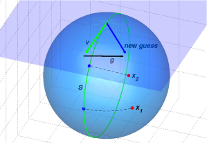
Figure 2: An iteration of Algorithm 2. The figure shows data points $x_{1}$ and $x_{2}$ (red points) with projections (blue points) to the geodesic subspace $S$ (green line). The vector $v$ defining $S$ is updated to the new guess by adding the gradient $g$ and normalizing.

4.4 Assumptions and Convergence

As discussed in section 2.4, because a uniqueness and existence of both the intrinsic mean and optima for (6) may fail, the PGA problem may not be well defined in itself. The uniqueness of the mean can be obtained by assuming the data is sufficiently concentrated depending on the curvature, see karcher_riemannian_1977 .

The curvature of the manifold may make the optimization problems non-convex, and convergence to a global optimum is therefore only ensured under the assumption that the problems (6) and (7) are convex or that no local minima exist. Giving criteria for convexity or non-existence of local optima for general manifolds and data sets is difficult because of the dependence on the global geometry of the manifolds.

The rank assumption on the Hessian used in Proposition 1 is equivalent to the residual $R_{x,\mu}$ having only non-degenerate critical points when restricted to $V_{v_{0}}$. It is shown in karcher_riemannian_1977 that $R_{x,\mu}$ is convex at points sufficiently close to $x$ and the assumption is therefore satisfied in such cases. In particular, this is satisfied if Algorithm 2 is initialized with subspaces that provide a good approximation to the data.

5 Experiments

We will use the optimization strategy and the developed algorithm for exact PGA to illustrate the differences between exact and linearized PGA. Furthermore, we will estimate sectional curvatures and compute injectivity radius bounds. Even though the algorithms are not limited to low dimensional data, we aim at visualizing the results and we will therefore provide examples with synthetic data on low dimensional manifolds. The setup allows exploring the connection between the geometry and curvature of the manifolds and the exact PGA result, and we will show how the variance and residual formulation can provide fundamentally different results. For a comparison between the methods on high dimensional manifolds modeling real-life data, we refer the reader to sommer_manifold_2010 where datasets of human vertebrae X-rays and motion capture data are treated.

The PGA algorithm is implemented in Matlab using Runge-Kutta ODE solvers. For the logarithm map, we use the shooting algorithm developed in sommer_bicycle_2009 . All tolerances used for the integration and logarithm calculations are set at or lower than an order of magnitude of the precision used for the displayed results. Intrinsic means are computed by iteratively minimizing variance using the gradient $\mathrm{grad}^{y}\|\mathrm{Log}_{y}x\|^{2}=-2\mathrm{Log}_{y}x$ (see karcher_riemannian_1977 ). The code used for the experiments is available at http://image.diku.dk/sommer.

We first consider surfaces embedded in $\mathbb{R}^{3}$ and defined by the equation

$$S_{c}=\{(x_{1},x_{2},x_{3})|cx_{1}^{2}+x_{2}^{2}+x_{3}^{2}=1\}$$

for different values of the scalar $c$. For $c>0$, $S_{c}$ is an ellipsoid and it is equal to $\mathbb{S}^{2}$ in the case $c=1$. The surface $S_{0}$ is a cylinder and, for $c<0$, $S_{c}$ is hyperboloid. Consider the point $p=(0,0,1)$ and note that $p\in S_{c}$ for all $c$. The curvature of $S_{c}$ at $p$ is equal to $c$. Note in particular that for the cylinder case the curvature is zero; the cylinder locally has the geometry of the plane $\mathbb{R}^{2}$ even though it informally seems to curve.

We evenly distribute 20 points along two straight lines through the origin of the tangent space $T_{p}S_{c}$, project the points from $T_{p}S_{c}$ to the surface $S_{c}$, and perform linearized and exact PGA. Figure 3 illustrates the situation in $T_{p}S_{-1}$ and on $S_{-1}$ embedded in $\mathbb{R}^{3}$, respectively. The lines are chosen in order to ensure the points are spread over areas of the surface with different geometry. This choice is made to illustrate the influence of the curvature; a more realistic example with points sampled from a Gaussian will be provided below.

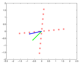
(a) $T_{p}S_{-1}$ with sampled points and first principal components (blue exact PGA, green linearized PGA).

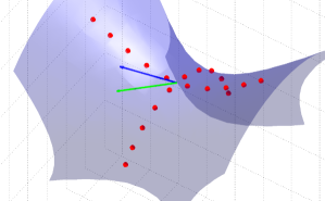
(b) $S_{-1}$ with projected points and first principal components (blue exact PGA (6), green linearized PGA).

Figure 3: The tangent space $T_{p}S_{-1}$ and the manifold $S_{-1}$ with sample points.

Since linearized PCA amounts to Euclidean PCA in $T_{p}S_{c}$, the first principal direction found using linearized PGA divides the angle between the lines for all $c$. In contrast to this, the variance and the first principal direction found using exact PGA are dependent on $c$. Table 1 shows the angle between the principal directions found using the two methods, the variances and variance differences for different values of $c$.

c:	1	0.5	0	-0.5	-1	-1.5	-2	-3	-4	-5
angle $(^{\circ})$:	0.0	0.1	0.0	22.3	29.2	31.5	32.6	33.8	34.2	34.5
linearized var.:	0.899	0.785	0.601	0.504	0.459	0.435	0.423	0.413	0.413	0.417
exact var.:	0.899	0.785	0.601	0.525	0.517	0.512	0.510	0.508	0.507	0.506
difference:	0.000	0.000	0.000	0.012	0.058	0.077	0.087	0.095	0.094	0.089
difference (%):	0.0	0.0	0.0	4.2	12.5	17.6	20.6	23.0	22.7	21.4

Table 1: Differences between methods for different values of $c$.

Let us give a brief explanation of the result. The symmetry of the sphere and the dataset cause the effect of curvature to even out in the spherical case $S_{1}$. The cylinder $S_{0}$ has local geometry equal to $\mathbb{R}^{2}$ which causes the equality between the methods in the $c=0$ case. The hyperboloids with $c<0$ that can be constructed by revolving a hyperbola around its semi-minor axis are non-symmetric causing an increase in variance as the first principal direction approaches the hyperbolic axis. The effect increases with the curvature causing the first principal direction to align with the hyperbolic axis for large negative values of $c$. That the non-linearity is quite complex can be seen from the decreasing differences for $c=-4,-5$, a consequence of the increasing variance captured using linearized PGA. This is caused by geodesics close to the semi-minor axis being curved upwards towards the hyperbolic axis for large negative $c$. This results in increased captured variance that dominates the otherwise decreasing trend as $c$ drops below $-3$. For all negative values of $c$, exact PGA is able to capture more variance in the subspace spanned by the first principal direction than linearized PGA.

Differences between the maximal variance PGA formulation (6) and the formulation that minimizes residual errors can be exemplified on simple geometries when the spread of the data is large. Similar examples for Geodesic PCA with variance formulation is reported huckemann_intrinsic_2010 . In Figure 4, points are sampled along a great circle through the north pole on a sphere ($c=1$). In order to illustrate the result of maximizing projection variance, we start with the PGA center point fixed to the north pole. In this case, each iteration of the optimization procedure pushes the first principal component $v^{1}$ away from the direction of the great circle. In fact, the optimal direction is orthogonal to the direction of the great circle. This very counter-intuitive effect is caused by the projection of the points on the southern hemisphere moving closer to the south pole as the principal subspaces moves away from the great circle thus causing the measured variance to increase. In fact, the cost function (6) is non-differentiable at the optimal direction and the projections become discontinuous functions of $v^{1}$. If we instead choose the formulation that minimizes residuals, the first principal component will align with the direction of the great circle.

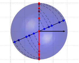
(a) Top view of the sphere $S_{1}$.

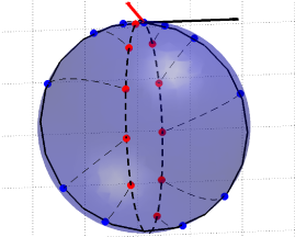
(b) Southern hemisphere of $S_{1}$.

Figure 4: The sphere $S_{1}$ with points (red) sampled along a great circle (black dotted circle) with tangent vector (red arrow). The optimization for the first principal component $v^{1}$ is stopped before it reaches its optimum (25 iterations). The actual optimum (black arrow) is orthogonal to the great circle containing the data points. The variance is measured for the points (blue) projected to the current guess for the first principal subspace (black circle). As the guess for $v^{1}$ moves away from being tangent to the circle containing the data points, points on the southern hemisphere move southwards causing the measured variance to increase.

To show that this effect persists under permutations of the data, we sample points uniformly along a geodesic on an ellipsoid ($c=0.5$) adding Gaussian noise on the component orthogonal to the geodesic (std. dev. $0.1$). This time, we optimize for the mean. The ellipsoidal geometry forces the mean to be close to the geodesic which is the reason for sampling on an ellipsoid; on a sphere, the mean is unstable under permutations of the data when the data lies close to a great circle. In Figure 5, we show the first principal component as computed with the variance and residual formulation, respectively. As for the example on the sphere, the optimization converges to a first principal component orthogonal to the geodesic with the variance formulation. We again stop the optimization after a number of iterations before it reaches its non-differentiable optimum. With the residual formulation, the first principal component aligns with the geodesic along which the points are sampled.

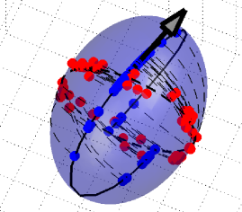
(a) First principal component (black arrow), variance formulation.

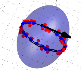
(b) First principal component (black arrow), residual formulation.

Figure 5: An ellipsoid $(c=0.5)$ with points (red) sampled uniformly along a geodesic (black dotted circle). Gaussian noise (std. dev. 0.1) is added to displace the points orthogonally to the geodesic. The black arrows show the result of the optimization with (a) the variance formulation and (b) the residual formulation. With the variance formulation, the optimization is again stopped before it reaches its non-differential optimum orthogonal to the geodesic along which the points are sampled. The results show that the orthogonality of the first principal component observed in Figure 4 also occurs with perturbed data.

See also huckemann_intrinsic_2010 for futher discussions on variance vs. residual formulations.

To investigate the difference between exact and linearized PGA with more than one principal direction, we consider a four dimensional manifold embedded in $\mathbb{R}^{5}$ and defined by

$$M_{4}=\{(x_{1},x_{2},x_{3},x_{4},x_{5})|x_{1}^{2}-2x_{2}^{2}+x_{3}^{2}-2x_{4}^{2}+x_{5}^{2}=1\}\ .$$

We make the situation more realistic than in the previous experiment by sampling 32 random points in the tangent space $T_{p}M_{4}$, $p=(0,0,0,0,1)$. Since $T_{p}M_{4}$ is an affine subspace of $\mathbb{R}^{5}$ orthogonal to the $x_{5}$ axis, we can identify it with $\mathbb{R}^{4}$ by the map $(x_{1},x_{2},x_{3},x_{4})\mapsto(x_{1},x_{2},x_{3},x_{4},1)$. We use this identification when sampling by defining a normal distribution in $\mathbb{R}^{4}$, sampling the 32 points from the distribution, and mapping the results to $T_{p}M_{4}$. The covariance is set to $\Sigma=\mbox{diag}(2,1,2/3,1/3)$ to get non-spherical distribution and to increase the probability of data spreading over high-curvature parts of the manifold. Table 2 lists the variances and variance differences for the four principal directions for both methods along with angular differences. The lower variance for exact PGA compared to the linearized method for the 2nd principal direction is due to the greedy definition of PGA; when maximizing variance for the 2nd principal direction, we keep the first principal direction fixed. Hence we may get lower variance than what is obtainable if we were to maximize for both principal directions together.

Princ. comp.:	1	2	3	4
angle $(^{\circ})$:	10.1	10.6	12.0	12.2
linearized var.:	1.58	3.86	4.13	4.35
exact var.:	1.93	3.85	4.24	4.35
difference:	0.35	-0.01	0.11	0.00
difference (%):	21.9	-0.3	2.6	0.0

Table 2: Differences between the methods on $M_{4}$. The variances of the data projected to the subspaces spanned by the first $k$ principal directions and the percentage and angular differences are shown for $k=1,\ldots,4$.

We clearly see angular differences between the principal directions. In addition, there is significant difference in accumulated variance in the first and third principal direction. We note that the percentage difference is calculated from what corresponds to the accumulated eigenspectrum in PCA. The percentage difference of the increase between the second and third principal direction, corresponding to the squared length of the third eigenvalue in PCA, is greater.

5.1 Curvature and Conjugate Points

Again considering the surfaces $S_{c}$, we can approximate the sectional curvature $K_{p}$ of $S_{c}$ at $p$ using (4). The approximation is dependent on the value of the positive scalar $t$ with increasing precision as $t$ decreases to zero. Table 3 shows the result of the sectional curvature approximation for two values of $t$ compared to the real sectional curvature.

c:	1	0	-1	-2	-3
$K_{p}$:	1	0	-1	-2	-3
$K_{p}$ est., $t=0.01$:	1.000	0.000	-1.000	-2.000	-3.000
$K_{p}$ est., $t=0.1$:	1.000	0.000	-1.001	-2.002	-3.005

Table 3: Sectional curvature at $p$ for different values of $c$.

Now let $J_{t}$ be the Jacobi field with $J_{0}=0$ and $\tfrac{D}{dt}J_{0}=(1,0,0)^{T}$ along the geodesic $x_{t}=\mathrm{Exp}_{p}t(0,1,0)^{T}$. Figure 6 shows $\|J_{t}\|$ for different values of $c$. We see that $\|J_{\pi}\|=0$ for the spherical case $S_{1}$ showing that $x_{1}$ is a conjugate point and hence giving the upper bound $\pi$ on the injectivity radius. The situation is illustrated in Figure 1. The local geometric equivalence between the cylinder $S_{0}$ and $\mathbb{R}^{2}$ causes the straight line for $c=0$. For all $c\leq 1$, the injectivity radius of $S_{c}$ is $\pi$, but for $c<1$, the point $x_{\pi}$ is not a conjugate point. By looking at $\|J_{t}\|$, we are only able to detect conjugate points and hence, with this experiment, we only get the bound on the injectivity radius for $c\geq 1$. For $c>1$ the injectivity radius decreases below $1$ as seen in the case $S_{2}$ with $\|J_{\tilde{t}}\|=0$ for $\tilde{t}\approx\pi/\sqrt{2}$.

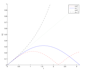
Figure 6: $\|J_{t}\|$ for $c=2,1,0,-1$ when $J_{0}=0$, $\tfrac{D}{dt}J_{0}=(1,0,0)^{T}$, and $x_{t}=\mathrm{Exp}_{p}t(0,1,0)^{T}$.

6 Conclusion and Outlook

Optimization problems over geodesics can be solved by constructing IVPs for numerical computation of Jacobi fields and second order differentials. We use this to develop an algorithm for numerically computing exact Principal Geodesic Analysis and thereby eliminating the need for the traditionally used linear approximations. In addition, the numerically computed Jacobi fields allow injectivity radii bounds and estimation of sectional curvatures partially solving an open problem stated in huckemann_intrinsic_2010 .

We use the developed algorithm to explore examples of manifold valued datasets where the principal subspaces computed by exact PGA differs from linearized PGA, and we show how the differences depend on the curvature of the manifolds and which formulation of PGA is used. In addition, we approximate sectional curvatures and bound injectivity radii and evaluate the computed results.

We are currently extending the methods to work for quotient manifolds $M/G$ and thereby allowing the similar computations to be performed on practically all commonly occurring non-triangulated manifolds. We expect this would allow Geodesic PCA to be computed on general quotient manifolds as well. In addition, we are working on giving a theoretical treatment of the differences between the variance and residual formulations of PGA. Finally, we expect to use the automatic computation of sectional curvatures to investigate further the effect of curvature on exact PGA and other statistical methods for manifold valued data.

Appendix A Notation

In general, the paper follows the notation in do_carmo_riemannian_1992 . Subscripts are used for curves on $M$ dependent on a parameter, e.g. the curve $\alpha_{t}$ is a map $(-\epsilon,\epsilon)\rightarrow M$. The subscript notation should not be confused with differentiation with respect to the parameter $t$. When a local parametrization $\mathbf{x}:U\subset\mathbb{R}^{\eta}\rightarrow M$ is available, it is often used to represent a curve $\alpha_{t}$ so that $x_{t}=(x^{1}_{t},\dots,x^{\eta}_{t})$ is a curve in $U$ satisfying $\mathbf{x}^{-1}\circ\alpha_{t}=x_{t}$.

The derivative $\tfrac{d}{dt}\alpha_{t}$ of the curve $\alpha_{t}$ evaluated at $\tilde{t}$ belongs to the tangent space $T_{\alpha_{\tilde{t}}}M$. The shorthand $\tfrac{d}{dt}\alpha_{\tilde{t}}$ will be used for such vectors, i.e. $\tfrac{d}{dt}\alpha_{t}|_{t=\tilde{t}}$. In addition, when differentiating curves with respect to $t$, we often use the shorthand $\dot{\alpha}_{t}$. With these conventions, $\tfrac{d}{dt}\alpha_{t}|_{t=0}$, the initial velocity of the curve $\alpha_{t}$, will be written $\dot{\alpha}_{0}$.

Let $df$ denote the differential of a map $f:M\to N$ and write $d_{p}f$ for the differential evaluated at $p\in M$. When bases for $T_{p}M$ and $T_{f(p)}M$ are specified, or when $M$ and $N$ are Euclidean spaces, $Df$ is used instead of $df$. For maps on product manifolds, e.g. $(v,w)\mapsto g(v,w):M\times\tilde{M}\to N$, we will need to distinguish differentiation with respect to one of the variables only. Letting one of the parameters have a fixed value $w_{0}$, the differential of the restricted function $v\mapsto g(v,w_{0})$ from $M$ to $N$ evaluated at $v_{0}$ is denoted $d^{v}_{(v_{0},w_{0})}g$. Similarly, if $V$ is a submanifold of $M$, the differential of $f|_{V}:V\to N$ will be denoted $d^{v\in V}f$ and its evaluation at $v_{0}\in V$ will be written $d^{v\in V}_{v_{0}}f$.

When defined, the inverse of the exponential map $\mathrm{Exp}_{q}$ is the logarithm map denoted $\mathrm{Log}_{q}(\tilde{q})$. Subsets $\mathrm{Exp}_{q}B_{r}(0)$ of $M$ with $B_{r}(0)$ being a ball in $T_{q}M$ and with the radius $r>0$ sufficiently small are examples of neighborhoods of $q$ in which $\mathrm{Log}_{q}(\tilde{q})$ is defined. Whenever the $\mathrm{Log}$-map is used, we will restrict to such neighborhoods without explicitly mentioning it.

When $h:M\to\mathbb{R}$ is a real valued function,the gradient of $h$ with respect to the metric is denoted $\mathrm{grad}\,h$, i.e. $\mathrm{grad}\,h$ satisfies $d_{p}h(v)=\left<\mathrm{grad}_{p}h,v\right>$ for all $v\in T_{p}M$. Whenever a basis of $T_{p}M$ is specified, or when $M$ is Euclidean, we switch to the usual notation $\nabla h$. Similarly, the Hessian of $h$ is defined by the relation $\text{Hessian}(h)X=\nabla_{X}\mathrm{grad}\,h$ for all vector fields $X$ using the covariant derivative $\nabla_{X}$. Again, when a basis of $T_{p}M$ is specified, or when $M$ is Euclidean, the usual notation $H(h)$ will be used.

Appendix B Expressions for the Derivative ODEs

Because we will work with curves on manifolds that are either embedded in a Euclidean space or where local parametrizations are available, we can perform the derivations needed for the differential systems in Euclidean spaces: the embedding space $\mathbb{R}^{m}$ for the implicit case, and the parameter space $U\subset\mathbb{R}^{\eta}$ when a parametrization $\mathbf{x}:U\rightarrow M$ is available. The tensors we construct below will be tensors on the Euclidean spaces $\mathbb{R}^{\eta}$ or $\mathbb{R}^{m}$; they will be used as a compact notational representations, and we do not attempt to give them intrinsic geometric interpretations. The tensors will be embedding or coordinate dependent; this is by construction, and the tensors are thereby inherently different from intrinsic and coordinate independent tensors such as the curvature endomorphism.

The notation will as far as possible follow the tensor notation used in do_carmo_riemannian_1992 ; however, we again note that we use the embedding or parametrization to define the tensors on Euclidean domains. We will use the common identification between tensors and multilinear maps, i.e. the tensor $T:(\mathbb{R}^{k})^{r}\rightarrow\mathbb{R}$ defines a map multilinear map $\tilde{T}:(\mathbb{R}^{k})^{r-1}\rightarrow\mathbb{R}^{k}$ by $\left<\tilde{T}(y_{1},\ldots,y_{r-1}),y_{r}\right>=T(y_{1},\ldots,y_{r})$. We will not distinguish between a tensor and its corresponding multilinear map, and hence, in the above case, write $T$ for both maps.

For $s$-dependent vector fields $v_{s,1},\ldots,v_{s,r}$ and tensor field $T_{s}$, we will use the equality

$$\begin{split}&\tfrac{d}{ds}T_{0}(v_{0,1},\ldots,v_{0,r})\\ &\quad=\left(\tfrac{d}{ds}T_{0}\right)(v_{0,1},\ldots,v_{0,r})+T_{0}(\tfrac{d}{ds}v_{0,1},\ldots,v_{0,r})+\cdots+T_{0}(y_{0,1},\ldots,\tfrac{d}{ds}v_{0,r})\end{split}$$ (22)

for the derivative with respect to $s$. If $T_{x_{s}}$ is a composition of an $z$-dependent tensor field $T_{z}$ and an $s$-dependent curve $x_{s}$, the derivative $\tfrac{d}{ds}T_{x_{s}}$ equals the covariant tensor derivative $\nabla_{\scriptscriptstyle\frac{d}{ds}x_{s}}T_{x_{s}}$ (do_carmo_riemannian_1992, , Chap. 4). Since we will only use tensors on Euclidean spaces, such tensor derivatives will consist of component-wise derivatives.

In the following, when a parametrization $\mathbf{x}$ is available, we let $T_{z}^{P}$ be the $z$-dependent $3$-tensor on $\mathbb{R}^{\eta}$ defined by

$$T_{z}^{P}(v_{1},v_{2},v_{3})=-\sum_{i,j,k}^{\eta}\Gamma_{ij}^{k}(z)v_{1}^{i}v_{2}^{j}v_{3}^{k}$$

such that the $k$th component of $T_{x_{t}}^{P}(\dot{x}_{t},\dot{x}_{t})$ equals the right hand side of (1). Note that $T_{z}^{p}$ is symmetric in the first two components since the Christoffel symbols are symmetric in $i$ and $j$. Similarly, in the implicit case, we let the $z$-dependent $3$-tensor $T_{z}^{I,p}$ and $2$-tensor $T_{z}^{I,x}$ equal the right hand side of the $p$ and $x$ parts of (2), respectively:

$$T_{z}^{I,p}(v_{1},v_{2})=-\left(\sum_{k=1}^{n}\mu^{k}(z,v_{1})H_{z}(F^{k})\right)v_{2}\ ,$$

$$T_{z}^{I,x}(v)=\left(I-D_{z}F^{\dagger}D_{z}F\right)v\ .$$

The derivation below of (10) concerns the implicit case.
 
To derive $F_{q,v}^{I}$, we let $x_{t,s}$ be a family of geodesics with $x_{t,0}=x_{t}$, and define $q_{s}=x_{0,s}$ and $v_{s}=\dot{x}_{0,s}$. Assuming $\tfrac{d}{ds}q_{0}=u$ and $\tfrac{d}{ds}v_{0}=w$, the Jacobi field $J_{t}$ equals $\tfrac{d}{ds}\mathrm{Exp}_{q_{s}}(tv_{s})|_{s=0}$, and, therefore, we can obtain $J_{t}$ by differentiating the geodesic system (2). Since $M$ is embedded in $\mathbb{R}^{m}$, we consider all curves and vectors to be elements of $\mathbb{R}^{m}$.

We use the map $\mu$ of section 2.2 to define the tensors

$$T_{z}^{\mu}(v)=\mu(z,v)\ ,\ T_{z}^{H}(v_{1},v_{2})=-\left(\sum_{k=1}^{n}v_{1}^{k}H_{z}(F^{k})\right)v_{2}\ ,$$

$$T_{z}^{D}(v)=\left(D_{z}F\right)v\ ,\mbox{ and }T_{z}^{D^{\dagger}}(v)=\left(D_{z}F\right)^{\dagger}v.$$

Note, in particular, that $T_{z}^{I,p}(v_{1},v_{2})=T_{z}^{H}(T_{z}^{\mu}(v_{1}),v_{2})$. In addition, we will use the notation $\Lambda(A,B)$ for the right hand side of equation (9) so that the derivative of a generalized inverse can be written $\tfrac{d}{ds}(A_{s}^{\dagger})=\Lambda(A_{s},\tfrac{d}{ds}A_{s})$. We claim that $\tfrac{d}{ds}\mathrm{Exp}_{q_{s}}(tv_{s})|_{s=0}$ equals the $z$-part of the solution of (10) with

$$\begin{split}&F_{q,v}^{I}\left(t,\begin{pmatrix}y_{t}\\ z_{t}\end{pmatrix}\right)\\ &\quad={\scriptstyle\begin{pmatrix}T_{x_{t}}^{I,p}(p_{t},\dot{z}_{t})+\nabla_{z_{t}}T_{x_{t}}^{H}(T_{x_{t}}^{\mu}(p_{t}),\dot{x}_{t})+T_{x_{t}}^{H}(T^{\mu}_{x_{t}}(y_{t})-\Lambda(T_{x_{t}}^{D},\nabla_{z_{t}}T_{x_{t}}^{D})^{T}p_{t},\dot{x}_{t})\ \\ T_{x_{t}}^{I,x}(y_{t})-\Lambda(T_{x_{t}}^{D},\nabla_{z_{t}}T_{x_{t}}^{D})T_{x_{t}}^{D}(p_{t})-T_{x_{t}}^{D^{\dagger}}\nabla_{z_{t}}T_{x_{t}}^{D}(p_{t})\end{pmatrix}}\ .\end{split}$$ (23)

Here $p_{t}=p_{t,0}$ where $p_{t,s}$ are the $p$-parts of the solutions to (2) with initial conditions $q_{s}$ and $v_{s}$. To justify the claim, we differentiate the system (2). Using (22), we get

$$\tfrac{d}{dt}\tfrac{d}{ds}p_{t,0}=\tfrac{d}{ds}\dot{p}_{t,0}=\tfrac{d}{ds}T_{x_{t,0}}^{I,p}(p_{t,0},\dot{x}_{t,0})$$

$$\qquad\quad\enspace=\nabla_{\scriptscriptstyle\frac{d}{ds}x_{t,0}}T_{x_{t}}^{H}(T_{x_{t}}^{\mu}(p_{t}),\dot{x}_{t})+T_{x_{t}}^{H}(\nabla_{\scriptscriptstyle\frac{d}{ds}x_{t,0}}T_{x_{t}}^{\mu}(p_{t})+T_{x_{t}}^{\mu}(\tfrac{d}{ds}p_{t,0}),\dot{x}_{t})$$

$$\qquad\qquad\enspace\,+T_{x_{t}}^{I,p}(p_{t},\tfrac{d}{ds}\dot{x}_{t,0})$$

and

$$\tfrac{d}{dt}\tfrac{d}{ds}x_{t,0}=\tfrac{d}{ds}\dot{x}_{t,0}=\tfrac{d}{ds}T_{t,0}^{I,x}(p_{t,0})=\nabla_{\scriptscriptstyle\frac{d}{ds}x_{t,0}}T_{x_{t}}^{I,x}(p_{t})+T_{x_{t}}^{I,x}(\tfrac{d}{ds}p_{t,0})\ .$$

Note that the tensor derivative $\nabla_{\scriptscriptstyle\frac{d}{ds}x_{t,0}}T_{x_{t}}^{H}$ consists of derivatives of $H_{x_{t}}(F^{k})$. Both the derivatives $\nabla_{\scriptscriptstyle\frac{d}{ds}x_{t,0}}T_{x_{t}}^{\mu}$ and $\nabla_{\scriptscriptstyle\frac{d}{ds}x_{t,0}}T_{x_{t}}^{I,x}$ involve derivatives of generalized inverses. Therefore, we apply (9) to differentiate $T_{x_{t}}^{\mu}$ and get that

$$\nabla_{\scriptscriptstyle\frac{d}{ds}x_{t,0}}T_{x_{t}}^{\mu}=-\Lambda(T_{x_{t}}^{D},\nabla_{\scriptscriptstyle\frac{d}{ds}x_{t,0}}T_{x_{t}}^{D})^{T}\ .$$

The tensor derivative $\nabla_{\scriptscriptstyle\frac{d}{ds}x_{t,0}}T_{x_{t}}^{D}$ consists of derivatives of $D_{x_{t,s}}F$. Similarly,

$$\nabla_{\scriptscriptstyle\frac{d}{ds}x_{t,0}}T_{x_{t}}^{I,x}=-\Lambda(T_{x_{t}}^{D},\nabla_{\scriptscriptstyle\frac{d}{ds}x_{t,0}}T_{x_{t}}^{D})T_{x_{t}}^{D}-T_{x_{t}}^{D^{\dagger}}\nabla_{\scriptscriptstyle\frac{d}{ds}x_{t,0}}T_{x_{t}}^{D}\ .$$

By differentiating the initial conditions, we get (10) with $y=\tfrac{d}{ds}p_{t,0}$, $z=\tfrac{d}{ds}x_{t,0}$, and $F_{q,v}^{I}$ as defined in (23).

As noted, we can obtain an IVP in the parametrized case using a similar procedure. Let $\alpha_{t}$ be a geodesic in the $C^{3}$ manifold $M$. We assume $\mathbf{x}:U\rightarrow M$ is a local parametrization containing $\alpha_{t}$, and we let $x_{t}$ be the curve in $U$ representing $\alpha_{t}$, i.e. $\mathbf{x}^{-1}\circ\alpha_{t}=x_{t}$. Let $\alpha_{0}=q$ and $\dot{\alpha}_{0}=v$, and let $u,w$ be vectors in $T_{q}M$. We associate $TM$ with $\mathbb{R}^{\eta}$ using $\mathbf{x}$. The Jacobi field $J_{t}$ along $\alpha_{t}$ with $J_{0}=u$ and $\tfrac{D}{dt}J_{0}=w$ can then be found as the $z$-part of the solution of the IVP

$$\begin{split}&\begin{pmatrix}\dot{y}_{t}\\ \dot{z}_{t}\end{pmatrix}=F_{q,v}^{P}\left(t,\begin{pmatrix}y_{t}\\ z_{t}\end{pmatrix}\right)\ ,\\ &\begin{pmatrix}y_{0}\\ z_{0}\\ \end{pmatrix}=\begin{pmatrix}w\\ u\end{pmatrix}\ ,\end{split}$$ (24)

with $F_{q,v}^{P}$ the map constructed below.

To derive $F_{q,v}^{P}$, we let $\alpha_{t,s}$ be a family of geodesics with $\alpha_{t,0}=\alpha_{t}$, and define $q_{s}=\alpha_{0,s}$ and $v_{s}=\dot{\alpha}_{0,s}$. Let $x_{t,s}$ represent $\alpha_{t,s}$ using $\mathbf{x}$. Again assuming $\tfrac{d}{ds}q_{0}=u$ and $\tfrac{d}{ds}v_{0}=w$, we can obtain $J_{t}$ by differentiating the geodesic system (1). Using (22) and symmetry of $T_{z}^{P}$, we have

$$\begin{split}&\tfrac{d}{dt^{2}}\tfrac{d}{ds}x_{t,0}=\tfrac{d}{ds}\ddot{x}_{t,0}=\tfrac{d}{ds}T_{x_{t,0}}^{P}(\dot{x}_{t,0},\dot{x}_{t,0})\\ &\qquad\qquad=\nabla_{\scriptscriptstyle\frac{d}{ds}x_{t,0}}T_{x_{t}}^{P}(\dot{x}_{t},\dot{x}_{t})+2T_{x_{t,0}}^{P}(\tfrac{d}{dt}\tfrac{d}{ds}x_{t,0},\dot{x}_{t})\ ,\\ &\tfrac{d}{ds}x_{0,0}=u,\ \tfrac{d}{dt}\tfrac{d}{ds}x_{0,0}=w\end{split}$$ (25)

because $x_{t,s}$ are solutions to (1) with initial conditions $q_{s}$ and $v_{s}$. Therefore, setting $y_{t}=\tfrac{d}{dt}\tfrac{d}{ds}x_{t,0}$ and $z_{t}=\tfrac{d}{ds}x_{t,0}$, we get (24) with

$$F_{q,v}^{P}(t,\begin{pmatrix}y_{t}\\ z_{t}\end{pmatrix})=\begin{pmatrix}\nabla_{z_{t}}T_{x_{t}}^{P}(\dot{x}_{t},\dot{x}_{t})+2T_{x_{t}}^{P}(y_{t},\dot{x}_{t})\\ y_{t}\end{pmatrix}\ .$$

As noted above, the derivative $\nabla_{\scriptscriptstyle\frac{d}{ds}x_{t,0}}T_{x_{s}}^{P}$ consists of just the component-wise derivatives of $T_{z}^{P}$, i.e. the derivatives of the Christoffel symbols.

For deriving the second order differentials, we will need second order derivatives of generalized inverses. Let $A_{t,s}$ be an $s$- and $t$-dependent matrix of full rank. From repeated application of the product rule and (9), we see that when the $s$- and $t$-dependent matrices $A_{t,s}$ and $A_{t,s}^{\dagger}$ are differentiable with respect to both variables and the mixed partial derivative $\tfrac{\partial^{2}}{\partial s\partial t}A_{t,s}$ exists then $\tfrac{\partial^{2}}{\partial s\partial t}(A_{t,s}^{\dagger})=\tilde{\Lambda}(A_{t,s},\tfrac{\partial}{\partial t}A_{t,s},\tfrac{\partial}{\partial s}A_{t,s},\tfrac{\partial^{2}}{\partial s\partial t}A_{t,s})$ where

$$\begin{split}&\tilde{\Lambda}(A,B,C,D)=-\Lambda(A,C)BA^{\dagger}-A^{\dagger}DA^{\dagger}-A^{\dagger}B\Lambda(A,C)-\Big{(}\Lambda(A,C)A+A^{\dagger}C\Big{)}B^{T}(A^{\dagger})^{T}A^{\dagger}\\ &\qquad\qquad\qquad\quad+(I-A^{\dagger}A)\Big{(}D^{T}(A^{\dagger})^{T}A^{\dagger}+B^{T}\big{(}\Lambda(A,C)^{T}A^{\dagger}+(A^{\dagger})^{T}\Lambda(A,C)\big{)}\Big{)}\ .\end{split}$$ (26)

We start the derivation with the parameterized case. We will use the tensors introduced in the beginning of this section and for the first order differentials.
 
We compute the $q$ and $r$ parts of $G_{q,v_{0},w,u}^{P}$ separately; denote them $G_{q,v_{0},w,u}^{P,q}$ and $G_{q,v_{0},w,u}^{P,r}$, respectively. Let $(y_{t,s}^{w},z_{t,s}^{w})$ be solutions to (24) with IV’s $(w,0)^{T}$ and along the curves $x_{t,s}$ that represents the geodesics $\alpha_{t,s}$. In addition, let $y_{t}^{w}$ and $z_{t}^{w}$ denote $y_{t,0}^{w}$ and $z_{t,0}^{w}$, respectively. Let also $(y_{t}^{u},z_{t}^{u})$ be solutions to $\eqref{sys:JP}$ with IV’s $(u,0)^{T}$ along $x_{t}=x_{t,0}$. Differentiating system (24), we get

$$\tfrac{d}{dt}\tfrac{d}{ds}(z_{t,0}^{w})=\tfrac{d}{ds}(\dot{z}_{t,0}^{w})=\tfrac{d}{ds}(y_{t,0}^{w})$$

and, using symmetry of the tensors,

$$\begin{split}&\tfrac{d}{dt}\tfrac{d}{ds}(y_{t,0}^{w})=\tfrac{d}{ds}(\dot{y}_{t,0}^{w})=\tfrac{d}{ds}\nabla_{z_{t,0}^{w}}T_{x_{t,0}}^{P}(\dot{x}_{t,0},\dot{x}_{t,0})+2\tfrac{d}{ds}T_{x_{t,0}}^{P}(y_{t,0}^{w},\dot{x}_{t,0})\\ &\qquad=\nabla_{z_{t}^{u}}\nabla_{z_{t}^{w}}T_{x_{t}}^{P}(\dot{x}_{t},\dot{x}_{t})+\nabla_{\scriptscriptstyle\frac{d}{ds}z_{t,0}^{w}}T_{x_{t}}^{P}(\dot{x}_{t},\dot{x}_{t})+2\nabla_{z_{t}^{w}}T_{x_{t}}^{P}(y_{t}^{u},\dot{x}_{t})\\ &\qquad\quad\,+2\nabla_{z_{t}^{u}}T_{x_{t}}^{P}(y_{t}^{w},\dot{x}_{t})+2T_{x_{t}}^{P}(\tfrac{d}{ds}y_{t,0}^{w},\dot{x}_{t})+2T_{x_{t}}^{P}(y_{t}^{w},y_{t}^{u})\ .\end{split}$$ (27)

Therefore, letting $q_{t}=\tfrac{d}{ds}y_{t,0}^{w}$ and $r_{t}=\tfrac{d}{ds}z_{t,0}^{w}$, we get $G_{q,v_{0},w,u}^{P,q}(t,(r_{t}\ q_{t})^{T})$ as the right hand side of (27) and $G_{q,v_{0},w,u}^{P,r}(t,(r_{t}\ q_{t})^{T})$ equal to $q_{t}$. The initial values are both $0$ since $y_{0,s}^{w}$ and $z_{0,s}^{w}$ equal $0$ and $w$, respectively, and, therefore, are not $s$-dependent.

For the implicit case, we will again compute the $r$ and $q$ parts of $G_{q,v_{0},w,u}^{I}$ separately. Let now $(y_{t,s}^{w},z_{t,s}^{w})$ be solutions to (10) along the geodesics $x_{t,s}$ and with IV’s $(w,0)^{T}$, and let $(y_{t}^{u},z_{t}^{u})$ be solutions to $\eqref{sys:JI}$ along $x_{t}$ and with IV’s $(u,0)^{T}$. Let also $p_{t,s}$ denote the $p$-parts of the solutions to (2) with initial conditions $q$ and $v_{s}$, and write $p_{t}=p_{t,0}$, $y_{t}^{w}=y_{t,0}^{w}$, and $z_{t}^{w}=z_{t,0}^{w}$. Recall that all curves and vectors are considered elements of the embedding space $\mathbb{R}^{m}$.

Differentiating system (10), we get

$$\tfrac{d}{dt}\tfrac{d}{ds}y_{t,0}^{w}=\tfrac{d}{ds}\dot{y}_{t,0}^{w}=\tfrac{d}{ds}T_{x_{t,0}}^{I,p}(p_{t,0},\dot{z}^{w}_{t,0})+\tfrac{d}{ds}\nabla_{z^{w}_{t,0}}T_{x_{t,0}}^{H}(T_{x_{t,0}}^{\mu}(p_{t,0}),\dot{x}_{t,0})$$

$$\qquad\qquad\qquad\qquad\enspace+\tfrac{d}{ds}T_{x_{t,0}}^{H}(T^{\mu}_{x_{t,0}}(y^{w}_{t,0})-\Lambda(T_{x_{t,0}}^{D},\nabla_{z^{w}_{t,0}}T_{x_{t,0}}^{D})^{T}p_{t,0},\dot{x}_{t,0})\ .$$

Using the map $\tilde{\Lambda}$ defined in (26), we have

$$\tfrac{d}{ds}\Lambda(T_{x_{t,0}}^{D},\nabla_{z^{w}_{t,0}}T_{x_{t,0}}^{D})^{T}=\tilde{\Lambda}(T_{x_{t}}^{D},\nabla_{z^{w}_{t}}T_{x_{t}}^{D},\nabla_{z^{u}_{t}}T_{x_{t}}^{D},\nabla_{z^{u}_{t}}\nabla_{z^{w}_{t}}T_{x_{t}}^{D})^{T}\ .$$

Combining the equations, we get

$$\tfrac{d}{dt}\tfrac{d}{ds}y_{t,0}^{w} =\nabla_{z^{u}_{t}}T_{x_{t}}^{I,p}(p_{t},\dot{z}^{w}_{t})+T_{x_{t}}^{I,p}(y^{u}_{t},\dot{z}^{w}_{t})+T_{x_{t}}^{I,p}(p_{t},\tfrac{d}{dt}\tfrac{d}{ds}z^{w}_{t,0})$$

$$\quad\,+\nabla_{z^{u}_{t}}\nabla_{z^{w}_{t}}T_{x_{t}}^{H}(T_{x_{t}}^{\mu}(p_{t}),\dot{x}_{t})+\nabla_{\tfrac{d}{ds}z^{w}_{t,0}}T_{x_{t}}^{H}(T_{x_{t}}^{\mu}(p_{t}),\dot{x}_{t})$$

$$\quad\,+\nabla_{z^{w}_{t}}T_{x_{t}}^{H}(T^{\mu}_{x_{t}}(y^{u}_{t})-\Lambda(T_{x_{t}}^{D},\nabla_{z^{u}_{t}}T_{x_{t}}^{D})^{T}p_{t},\dot{x}_{t})+\nabla_{z^{w}_{t}}T_{x_{t}}^{H}(T_{x_{t}}^{\mu}(p_{t}),\dot{z}^{u}_{t})$$

$$\quad\,+\nabla_{z^{u}_{t}}T_{x_{t}}^{H}(T^{\mu}_{x_{t}}(y^{w}_{t})-\Lambda(T_{x_{t}}^{D},\nabla_{z^{w}_{t}}T_{x_{t}}^{D})^{T}p_{t},\dot{x}_{t})$$

$$\quad\,+T_{x_{t}}^{H}(T^{\mu}_{x_{t}}(\tfrac{d}{ds}y^{w}_{t,0})-\Lambda(T_{x_{t}}^{D},\nabla_{z^{u}_{t}}T_{x_{t}}^{D})^{T}y^{w}_{t},\dot{x}_{t})$$

$$\quad\,-T_{x_{t}}^{H}(\tilde{\Lambda}(T_{x_{t}}^{D},\nabla_{z^{w}_{t}}T_{x_{t}}^{D},\nabla_{z^{u}_{t}}T_{x_{t}}^{D},\nabla_{z^{u}_{t}}\nabla_{z^{w}_{t}}T_{x_{t}}^{D})^{T}p_{t}+\Lambda(T_{x_{t}}^{D},\nabla_{z^{u}_{t}}T_{x_{t}}^{D})^{T}y^{u}_{t},\dot{x}_{t})$$

$$\quad\,+T_{x_{t}}^{H}(T^{\mu}_{x_{t}}(y^{w}_{t})-\Lambda(T_{x_{t}}^{D},\nabla_{z^{w}_{t}}T_{x_{t}}^{D})^{T}p_{t},\dot{z}^{u}_{t})\ .$$

Substituting $\tfrac{d}{ds}z_{t,0}^{w}$ with $r_{t}$ and $\tfrac{d}{ds}y_{t,0}^{w}$ with $q_{t}$, we get $G_{q,v_{0},w,u}^{I,q}$ as the right hand side of the equation. Likewise,

$$\tfrac{d}{dt}\tfrac{d}{ds}z_{t,0}^{w} =\tfrac{d}{ds}T_{x_{t,0}}^{I,x}(y^{w}_{t,0})-\tfrac{d}{ds}\Lambda(T_{x_{t,0}}^{D},\nabla_{z^{w}_{t,0}}T_{x_{t,0}}^{D})T_{x_{t,0}}^{D}(p_{t,0})-\tfrac{d}{ds}T_{x_{t,0}}^{D^{\dagger}}\nabla_{z^{w}_{t,0}}T_{x_{t,0}}^{D}(p_{t,0})$$

$$=\nabla_{z^{u}_{t}}T_{x_{t}}^{I,x}(y^{w}_{t})+T_{x_{t}}^{I,x}(\tfrac{d}{ds}y^{w}_{t,0})$$

$$-\tilde{\Lambda}(T_{x_{t}}^{D},\nabla_{z^{w}_{t}}T_{x_{t}}^{D},\nabla_{z^{u}_{t}}T_{x_{t}}^{D},\nabla_{z^{u}_{t}}\nabla_{z^{w}_{t}}T_{x_{t}}^{D})T_{x_{t}}^{D}(p_{t})$$

$$-\Lambda(T_{x_{t}}^{D},\nabla_{z^{w}_{t}}T_{x_{t}}^{D})\nabla_{z^{u}_{t}}T_{x_{t}}^{D}(p_{t})-\Lambda(T_{x_{t}}^{D},\nabla_{z^{w}_{t}}T_{x_{t}}^{D})T_{x_{t}}^{D}(y^{u}_{t})$$

$$-\Lambda(T_{x_{t}}^{D},\nabla_{z^{u}_{t}}T_{x_{t}}^{D})\nabla_{z^{w}_{t}}T_{x_{t}}^{D}(p_{t})-T_{x_{t}}^{D^{\dagger}}\nabla_{z^{u}_{t}}\nabla_{z^{w}_{t}}T_{x_{t}}^{D}(p_{t})-T_{x_{t}}^{D^{\dagger}}\nabla_{z^{w}_{t}}T_{x_{t}}^{D}(y^{u}_{t})\ .$$

Again, after substituting $\tfrac{d}{ds}y_{t,0}^{w}$ with $q_{t}$ as above, we get $G_{q,v_{0},w,u}^{I,r}$ as the right hand side of the equation. As for the parametric case, both initial values are zero.

Appendix C The Projection Differential

For the proof of Proposition 1, we will need the following result to show that equation (15) is independent of the chosen basis.

Lemma 1

Let $S$ be an open subset of $\mathbb{R}^{k}$ and $U:S\rightarrow M^{k\times(k-1)}$ a $C^{1}$ map with the property that for any $v\in S$, the columns of the matrix $(\tfrac{v}{\|v\|}\ U(v))$ constitute an orthonormal basis for $\mathbb{R}^{k}$. Let $u_{v}^{j}$ denote the $j$th column of $U(v)$. Then for any $v_{0}\in S$ and $w\in\mathbb{R}^{k}$, $\left<\tfrac{d}{dt}u_{v_{0}+tw}^{j}|_{t=0},v_{0}\right>=-\left<u_{v_{0}}^{j},w\right>$. As consequence of this, if $\tilde{U}:S\rightarrow\mathbb{R}^{k-1}$ denotes the map $v\mapsto U(v)^{T}\tfrac{v_{0}}{\|v_{0}\|}$ then

$$D^{v\in\mathrm{span}\,(u_{v_{0}}^{1},\ldots,u_{v_{0}}^{k-1})}_{v_{0}}\tilde{U}(v)=-I_{k-1}$$

in the basis $u_{v_{0}}^{1},\ldots,u_{v_{0}}^{k-1}$ for $\mathrm{span}\,(u_{v_{0}}^{1},\ldots,u_{v_{0}}^{k-1})$.

References

- (1) Harry Blum and Weiant Wathen-Dunn, A Transformation for Extracting New Descriptors of Shape, Models for the Perception of Speech and Visual Form (1967), 362–380.
- (2) Vicent Caselles, Ron Kimmel, and Guillermo Sapiro, Geodesic Active Contours, International Journal of Computer Vision 22 (1995), 61—79.
- (3) Henry P. Decell, On the derivative of the generalized inverse of a matrix, Linear and Multilinear Algebra 1 (1974), no. 4, 357.
- (4) Jean-Pierre Dedieu and Dmitry Nowicki, Symplectic methods for the approximation of the exponential map and the Newton iteration on Riemannian submanifolds, Journal of Complexity 21 (2005), no. 4, 487–501.
- (5) Manfredo Perdigao do Carmo, Riemannian geometry, Mathematics: Theory & Applications, Birkhauser Boston Inc., Boston, MA, 1992.
- (6) Ricardo Ferreira, Joao Xavier, Joaoa Costeria, and Victor Barroso, Newton Algorithms for Riemannian Distance Related Problems on Connected Locally Symmetric Manifolds, Technical Report, Institute for Systems and Robotics (ISR) (2008).
- (7) P. Thomas Fletcher and Sarang Joshi, Principal geodesic analysis on symmetric spaces: Statistics of diffusion tensors, ECCV Workshops CVAMIA and MMBIA. 3117 (2004), 87—98.
- (8) , Riemannian geometry for the statistical analysis of diffusion tensor data, Signal Processing 87 (2007), no. 2, 250–262.
- (9) P. Thomas Fletcher, Suresh Venkatasubramanian, and Sarang Joshi, Robust statistics on Riemannian manifolds via the geometric median, 2008 IEEE Conference on Computer Vision and Pattern Recognition (Anchorage, AK, USA), June 2008, pp. 1–8.
- (10) PT Fletcher, Geodesic Regression on Riemannian Manifolds, Workshop on Mathematical Foundations of Computational Anatomy (MFCA) at MICCAI, 2011.
- (11) P.T. Fletcher, Conglin Lu, and S. Joshi, Statistics of shape via principal geodesic analysis on Lie groups, CVPR 2003, vol. 1, 2003, pp. I–95–I–101 vol.1.
- (12) P.T. Fletcher, Conglin Lu, S.M. Pizer, and Sarang Joshi, Principal geodesic analysis for the study of nonlinear statistics of shape, Medical Imaging, IEEE Transactions on (2004).
- (13) M. Fréchet, Les éléments aléatoires de nature quelconque dans un espace distancie, Ann. Inst. H. Poincaré 10 (1948), 215–310.
- (14) G. H. Golub and V. Pereyra, The Differentiation of Pseudo-Inverses and Nonlinear Least Squares Problems Whose Variables Separate, SIAM Journal on Numerical Analysis 10 (1973), no. 2, 413–432.
- (15) Ernst Hairer, Christian Lubich, and Gerhard Wanner, Geometric numerical integration, Springer, 2002.
- (16) Ernst Hairer, Syvert P. Nørsett, and Gerhard Wanner, Solving Ordinary Differential Equations I: Nonstiff Problems (Springer Series in Computational Mathematics), 2nd ed., Springer, May 2008.
- (17) Richard J. Hanson and Charles L. Lawson, Extensions and Applications of the Householder Algorithm for Solving Linear Least Squares Problems, Mathematics of Computation 23 (1969), no. 108, 787–812.
- (18) Søren Hauberg, Stefan Sommer, and Kim Steenstrup Pedersen, Natural metrics and least-committed priors for articulated tracking, Image and Vision Computing 30 (2012), no. 6–7.
- (19) Stephan Huckemann, Thomas Hotz, and Axel Munk, Intrinsic shape analysis: Geodesic PCA for Riemannian manifolds modulo isometric Lie group actions, Statistica Sinica 20 (2010), no. 1, 1–100.
- (20) Sarang Joshi, Stephen Pizer, P Thomas Fletcher, Paul Yushkevich, Andrew Thall, and J S Marron, Multiscale deformable model segmentation and statistical shape analysis using medial descriptions, IEEE Transactions on Medical Imaging 21 (2002), no. 5, 538–550, PMID: 12071624.
- (21) H. Karcher, Riemannian center of mass and mollifier smoothing, Communications on Pure and Applied Mathematics 30 (1977), no. 5, 509–541.
- (22) Herbert Bishop Keller, Numerical methods for two-point boundary-value problems, Blaisdell, (Waltham, Mass), 1968.
- (23) David G. Kendall, Shape Manifolds, Procrustean Metrics, and Complex Projective Spaces, Bull. London Math. Soc. 16 (1984), no. 2, 81–121.
- (24) Eric Klassen and Anuj Srivastava, Geodesics Between 3D Closed Curves Using Path-Straightening, ECCV 2006, vol. 3951, Springer, 2006, pp. 95–106.
- (25) Eric Klassen, Anuj Srivastava, Washington Mio, and Shantanu Joshi, Analysis of planar shapes using geodesic paths on shape spaces, IEEE Transactions on Pattern Analysis and Machine Intelligence 26 (2004), 372—383.
- (26) John M Lee, Riemannian manifolds, Graduate Texts in Mathematics, vol. 176, Springer-Verlag, New York, 1997.
- (27) David G. Luenberger, The Gradient Projection Method along Geodesics, Management Science 18 (1972), no. 11, 620–631.
- (28) Lyle Noakes, A Global Algorithm for Geodesics, Journal of the Australian Mathematical Society 64 (1998), 37–50.
- (29) Xavier Pennec, Intrinsic Statistics on Riemannian Manifolds: Basic Tools for Geometric Measurements, J. Math. Imaging Vis. 25 (2006), no. 1, 127–154.
- (30) Xavier Pennec, Pierre Fillard, and Nicholas Ayache, A Riemannian Framework for Tensor Computing, Int. J. Comput. Vision 66 (2006), no. 1, 41–66.
- (31) Xavier Pennec, Charles Guttmann, and Jean-Philippe Thirion, Feature-based registration of medical images: Estimation and validation of the pose accuracy, MICCAI 1998, Springer Berlin, 1998, pp. 1107–1114.
- (32) Patrick J. Rabier and Werner C. Rheinboldt, On a computational method for the second fundamental tensor and its application to bifurcation problems, Numerische Mathematik 57 (1990), no. 1, 681–694.
- (33) W. C. Rheinboldt, MANPAK: A set of algorithms for computations on implicitly defined manifolds, Computers & Mathematics with Applications 32 (1996), no. 12, 15–28.
- (34) Salem Said, Nicolas Courty, Nicolas Le Bihan, and Stephen Sangwine, Exact Principal Geodesic Analysis for Data on SO(3), EUSIPCO 2007 (2007).
- (35) Frank Schmidt, Michael Clausen, and Daniel Cremers, Shape Matching by Variational Computation of Geodesics on a Manifold, Pattern Recognition, Springer Berlin, 2006, pp. 142–151.
- (36) Cristian Sminchisescu and Allan Jepson, Generative Modeling for Continuous Non-Linearly Embedded Visual Inference, In ICML (2004), 759—766.
- (37) Stefan Sommer, Horizontal Dimensionality Reduction and Iterated Frame Bundle Development, Geometric Science of Information (GSI), 2013.
- (38) Stefan Sommer, Francois Lauze, Søren Hauberg, and Mads Nielsen, Manifold Valued Statistics, Exact Principal Geodesic Analysis and the Effect of Linear Approximations, ECCV 2010, vol. 6316, Springer, 2010.
- (39) Stefan Sommer, Aditya Tatu, Chen Chen, Dan Jørgensen, Marleen de Bruijne, Marco Loog, Mads Nielsen, and Francois Lauze, Bicycle chain shape models, MMBIA workshop at CVPR, 2009.
- (40) Raquel Urtasun, David J. Fleet, Aaron Hertzmann, and Pascal Fua, Priors for People Tracking from Small Training Sets, 2005 IEEE International Conference on Computer Vision (ICCV), IEEE Computer Society, 2005, pp. 403–410.
- (41) Jing Wu, W. Smith, and E. Hancock, Weighted Principal Geodesic Analysis for Facial Gender Classification, Progress in Pattern Recognition, Image Analysis and Applications, Springer Berlin, 2008, pp. 331–339.
- (42) Le Yang, Means of probability measures in Riemannian manifolds and applications to radar target detection, Ph.D. thesis, Poitiers University, 2011.
- (43) Y. Yang, Globally Convergent Optimization Algorithms on Riemannian Manifolds: Uniform Framework for Unconstrained and Constrained Optimization, Journal of Optimization Theory and Applications 132 (2007), no. 2, 245–265.
- (44) Laurent Younes, Felipe Arrate, and Michael I. Miller, Evolutions equations in computational anatomy, NeuroImage 45 (2009), no. 1, Supplement 1, S40–S50.
- (45) Qin Zhang and Guoliang Xu, Curvature computations for n-manifolds in and solution to an open problem proposed by R. Goldman, Computer Aided Geometric Design 24 (2007), no. 2, 117–123.