Transport in the $3$-dimensional Anderson model:
an analysis of the dynamics on scales below the localization length

Abstract

Single-particle transport in disordered potentials is investigated on scales below the localization length. The dynamics on those scales is concretely analyzed for the $3$-dimensional Anderson model with Gaussian on-site disorder. This analysis particularly includes the dependence of characteristic transport quantities on the amount of disorder and the energy interval, e.g., the mean free path which separates ballistic and diffusive transport regimes. For these regimes mean velocities, respectively diffusion constants are quantitatively given. By the use of the Boltzmann equation in the limit of weak disorder we reveal the known energy-dependencies of transport quantities. By an application of the time-convolutionless (TCL) projection operator technique in the limit of strong disorder we find evidence for much less pronounced energy dependencies. All our results are partially confirmed by the numerically exact solution of the time-dependent Schrödinger equation or by approximative numerical integrators. A comparison with other findings in the literature is additionally provided.

1 Introduction

Any solid contains disorder: Either there are impurities, vacancies, and dislocations in an otherwise ideal crystal lattice. Or there is no lattice structure at all. An abstract quantum system which is commonly used as a paradigm for transport in real disordered solids is the Anderson model [1]. In its probably simplest form without particle-particle interactions (electron-electron, electron-phonon, etc.) the Hamiltonian may be written as

$$\hat{H}=\sum_{\vec{r}}\epsilon_{\vec{r}}\,\,\hat{a}^{\dagger}_{\vec{r}}\,\hat{a}_{\vec{r}}+\sum_{\textnormal{NN}}\hat{a}^{\dagger}_{\vec{r}_{1}}\hat{a}_{\vec{r}_{2}}\,,$$ (1)

where $\hat{a}_{\vec{r}}$ and $\hat{a}^{\dagger}_{\vec{r}}$ denote the usual annihilation, respectively creation operators; $\vec{r}$ labels the sites of a $d$-dimensional (cubic) lattice; NN indicates a sum over nearest neighbors $\vec{r}_{1}$ and $\vec{r}_{2}$; and $\epsilon_{\vec{r}}$ represent independent random numbers, e.g., according to a Gaussian distribution with mean $\langle\epsilon_{\vec{r}}\rangle=0$ and variance $\langle\epsilon_{\vec{r}_{1}}\,\epsilon_{\vec{r}_{2}}\rangle=\delta_{\vec{r}_{1},\vec{r}_{2}}\,\sigma^{2}$. Even though such a distribution is considered throughout this work, the random numbers can be realized according to a Lorentzian, box, or binary distribution as well [2, 3, 4]. In all cases disorder is implemented in terms of a random on-site potential. (Random hopping coefficients are sometimes taken into account, too.)
In the presence of such a disorder, $\sigma\neq 0$, the eigenstates of the Hamiltonian are no longer given by Bloch functions: Instead the eigenstates are not necessarily extended over the whole lattice and can become localized in configuration space, i.e., the envelope of a wavefunction decays exponentially on a finite localization length [2, 5]. The finiteness of the localization length is one manifestation and, say, definition of the localization phenomenom. (There certainly are other mathematical definitions of localization, e.g., the finiteness of the inverse participation number, the independence of eigenvalues from boundary conditions, etc. [2]) This phenomenon and particularly its impact on transport have intensively been studied for the Anderson model [1, 2, 3, 4, 5, 6, 7, 8, 9, 10].
For the lower dimensional cases, $d=1$ and $d=2$, all eigenstates of the Hamiltonian feature finite localization lengths for arbitrary (non-zero) values of $\sigma$ (except for situations with short-range correlated disorder, e.g., as realized in the random dimer model [11, 12]). Therefore in the thermodynamic limit, i.e., with respect to the infinite length scale an insulator is to be expected. Of particular interest is the $3$-dimensional case, as considered in the work at hand. Here, a mobility edge, i.e., a certain cross-over energy separates the spatially localized from the spatially extended wavefunctions in energy space [2, 3, 5]. When the amount of disorder is increased, the mobility edge goes above the Fermi level and a metal-to-insulator transition is induced at zero temperature, still with respect to the infinite length scale. When $\sigma$ is further increased above the critical disorder ($\sigma_{C}\approx 6$ for a Gaussian distribution [2, 3, 4]), all eigenstates become localized and an insulator is to be expected for each temperature (without particle-particle interactions). The Anderson metal-to-insulator transition is widely believed to be continuous without a minimum conductivity, e.g., as supported by the one-parameter scaling theory of localization [2, 5, 7].
Our work, other than most of the pertinent literature, focuses on the dynamics on scales below the localization length. We particularly intend to analyze the dynamics on those scales comprehensively as a function of energy and disorder. Qualitatively, our analysis allows to identify two regimes of length scales which are purely ballistic and strictly diffusive (rather than superdiffusive, subdiffusive, or anything else). It generally is a challenge to theoretically confirm reliably the “presence of diffusion” in strongly disordered and/or interacting quantum systems. Quantitatively, our analysis enables the evaluation of mean velocities, respectively diffusion coefficients for a wide range of disorders between zero and the vicinity of $\sigma_{C}$. Such a detailed knowledge about diffusion constants appears to be important, especially since dc-conductivities are directly related by the Einstein relation, at least for $\sigma<\sigma_{C}$. In the limit of strong disorder diffusion coefficients have been suggested in the literature by the numerical study of Green’s functions for very few disorders and a single energy at the spectral middle solely [8, 9]. The dependence of diffusion constants on energy is usually discussed in the limit of weak disorder only. However, also in that limit, we demonstrate that energy dependencies are much richer than common approximations for a free electron gas [2].
The work at hand is structured as follows: First of all we provide a qualitative picture of the dynamics on scales below the localization length in section 2. Then this qualitative picture is subsequently developed and quantitatively confirmed in the whole section 3: The limit of weak disorder is firstly analyzed in section 3.1 by the use of the Boltzmann equation [13, 14, 15, 16]. The limit of strong disorder is afterwards investigated by an application of a method which is mainly based on the time-convolutionless (TCL) projection operator technique [17, 18, 19, 20, 21]. In section 3.2 the method as such is introduced and its predictions on the dynamics are presented. The validity range of these predictions is analytically discussed in section 3.3 and numerically verified in section 3.4. We finally close with a summary and conclusion in section 4.

2 Qualitative picture of the dynamics

In the present section we intend to provide firstly a qualitative picture of the dynamics on scales below the localization length. This qualitative picture essentially summarizes the findings of the methods which are introduced in detail and applied concretely in the following sections. In particular we emphasize the main conclusions of the work at hand and discuss these conclusions in the context of known results in the literature. In this way we also give a comprehensive summary for the readers which are not primarily interested in the methodic details. Apart from that the summary certainly makes the line of thoughts in the subsequent sections more plainly.
The above mentioned qualitative picture of the dynamics is illustrated in figure 1.

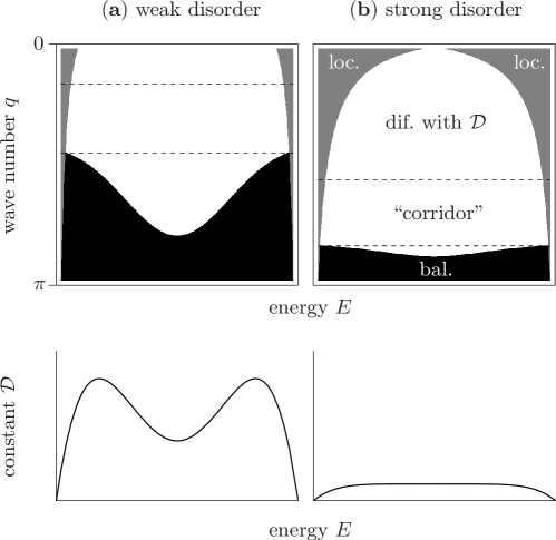
Figure 1: Sketch for the dependence of transport on the wave number $q$ and the energy $E$ for (a) weak disorder and (b) strong disorder. Both top panels indicate the rough position of localized (loc., gray), diffusive (dif., white) and ballistic (bal., black) regimes. Particularly, a possible “corridor” of wave numbers is indicated (dashed lines), where transport is diffusive for almost all energies. Both bottom panels display suggestions for qualitatively different energy dependencies of the diffusion constant.

In this figure a sketch for the dependence of transport on the length scale $l$, respectively wave number $q$ and the energy $E$ is shown for the two cases of (a) weak disorder and (b) strong disorder. For both cases the sketch indicates the rough position of the different transport regimes, namely, localized (loc., gray), diffusive (dif., white), and ballistic (bal., black).
It is well known that in the limit of weak disorder the localization phenomenon is restricted to the borders of the spectrum solely. Deep in the outer tails of the spectrum the states are localized on a single lattice site, whereas the overwhelming majority of all states, i.e., not only the ones from the spectral middle, is still extended. Thus, as displayed in figure 1, the localization length (envelope of gray areas) is not a closed curve in the $(q,E)$-space. The energies which separate localized and non-localized regimes at $q=0$ (points between gray and white areas at $q=0$) are the mobility edges. And in fact, much work has been devoted to the concrete position of the mobility edges [2, 3]. Only for energies between the mobility edges there is a conductor at the infinite length scale, otherwise there is an insulator at that length scale, of course. But, as already mentioned before, insulating behavior is practically absent in the limit of weak disorder, e.g., the Fermi level is much larger than the lower mobility edge.
While insulating behavior appears at rather large length scales above the localization length, ballistic behavior occurs at comparatively small length scales below the mean free path (envelope of black area). Here, (quasi-)particles are not scattered and move freely with mean (group) velocities, e.g., as routinely evaluated in the framework of standard solid state theory. The latter free motion is reflected in the term ballistic and is typical for an ideal conductor. The mean free path, as drawn in figure 1, appears to be a contra-intuitive curve in the $(q,E)$-space, since it is smaller for states from the spectral middle than for states from the borders of the spectrum. However, we demonstrate in section 3.1 that in the limit of weak disorder such a curve results from the Boltzmann equation.
Apparently, for weak disorder there is the practically unbounded regime above the mean free path where transport is neither insulating nor ballistic. This is the regime where transport is generally expected to be diffusive, i.e., at that length scales one expects a normal conductor. Particularly, figure 1 marks a “corridor” of wave numbers (dashed lines) with diffusive dynamics at almost all energies. (The notion of a diffusive corridor becomes helpful for later argumentations in the context of strong disorder where the existence of such a corridor is anything else than obvious.) From a mere theoretical point of view it is a challenge to concisely show that the dynamics is in full accord with a diffusion equation. But in section 3.1 we demonstrate by the use of the Boltzmann equation that the dynamics is indeed diffusive and further evaluate quantitatively the diffusion coefficient as a function of energy. As indicated in figure 1, its dependence on energy seems to be as contra-intuitive as the one of the mean free path and strongly differs in the details from the approximations according to a free electron gas.
For strong disorder the localization phenomenon is much more pronounced. When the amount of disorder is increased, the localized regimes gradually expand towards small length scales and towards energies in the middle of the spectrum as well, see figure 1. On the one hand the already non-extended states become localized on smaller and smaller length scales. On the other hand more and more of the before extended states become localized at all. Hence, the mobility edges move closer to each other and eventually meet, once the critical disorder is reached. Then all states are localized and transport at the infinite length scale vanishes completely, i.e., at all energies. Therefore much work has addressed the concrete evaluation of the critical disorder [2, 3, 4]. However, even above the critical disorder, transport takes place below the localization length, of course.
It is a priori not clear whether or not the dynamics below the localization length is still in good agreement with a diffusion equation in the limit of strong disorder, both below and above the critical disorder. But by the use of a method which is based on the TCL projection operator technique we demonstrate in section 3.2 that there also exists a corridor of wave numbers where the dynamics is indeed diffusive at almost all energies, at least as long as the amount of disorder does not become too strong. In particular the diffusion constant within this corridor does not substantially depend on energy, see figure 1. In fact, only if the dynamics for a certain wave number is not governed by a significant energy dependence, the method makes a definite conclusion, otherwise no information results except for the strong energy dependence of the dynamics, e.g., the method can not distinguish between highly energy dependent diffusion coefficients and non-negligible localized contributions. However, once a diffusive corridor of wave numbers with a single diffusion constant is reliably detected, it is natural to assume that the diffusion coefficient does not change, when this corridor is left. (Per definition diffusion coefficients should not depend on the wave number). Or, in other words, we suggest that in the limit of strong disorder the dynamics in the whole diffusive regime is well described by an energy independent diffusion constant. This diffusion constant is quantitatively evaluated in section 3.2 as a function of disorder.
For the case of strong disorder the TCL-based method additionally allows to characterize the ballistic regime, i.e., by the use of the method the mean free path and the mean velocity can be also evaluated. Similarly, these quantities are found to be approximately independent from energy. This observation suggests that in the limit of strong disorder the whole dynamics below the localization length is not governed by significant energy dependencies. Of course, in a sense this suggestion disagrees with the observations for the case of weak disorder. Nevertheless, in the sections 3.1 and 3.2 the disagreement is subsequently resolved, both qualitatively and quantitatively.

3 Quantitative results

3.1 Weak disorder: Boltzmann equation

In the present section we are going to investigate the dynamics in the limit of weak disorder. In that limit there certainly is a large variety of different approaches which all treat the disorder as a small perturbation to the clean Hamiltonian. Here, we briefly review on one class of these approaches, namely, the mapping of the quantum dynamics onto Boltzmann equations [13, 14, 15, 16]. Different approaches to such a map rely on different assumptions and/or approximation schemes which are not entirely free of their own subtleties. However, the particle velocities that eventually enter the Boltzmann equation are routinely taken from the clean (unperturbed) Hamiltonian. To this end the clean Hamiltonian has to be diagonalized at first. Routinely, this diagonalization can be done by the application of the Fourier transform. Then the Hamiltonian takes on the form

$$\hat{H}=\sum_{\vec{q}}\,E_{\vec{q}}\,\,\hat{a}^{\dagger}_{\vec{q}}\,\hat{a}_{\vec{q}}\,,$$ (2)

where $\hat{a}^{\dagger}_{\vec{q}}$, $\hat{a}_{\vec{q}}$ are creation, annihilation operators for (quasi-)particles with the wave vector $\vec{q}$, i.e., $q_{i}=2\pi\,k_{i}/N$, $k_{i}=0,\ldots,N-1$. The corresponding dispersion relation reads

$$E_{\vec{q}}=\sum_{i=1}^{3}\,2\,(1-\cos q_{i})\approx|\,\vec{q}\,|^{2}\,.$$ (3)

(Now and in the following the indicated approximations hold true for sufficiently small $|\,\vec{q}\,|$, respectively low energies and are well known from the free electron gas.) As long as disorder is absent, the (quasi-)particles are not scattered and may be said to move freely with the (group) velocities which are determined by the derivative of the dispersion relation, namely,

$$v_{\vec{q}}=|\,\nabla_{\!\vec{q}}\,E_{\vec{q}}\,|=2\,\sqrt{\sum_{i=1}^{3}\,\sin^{2}q_{i}}\approx 2\,|\,\vec{q}\,|\,.$$ (4)

Whithin such a Boltzmann equation framework disorder takes the role of a set of impurities from which the (quasi-)particles are scattered after, say, a mean free time $\tau(E)$, respectively mean free path $l(E)$. Therefore disorder essentially gives raise to a linear collision term, i.e., a rate matrix which describes the transitions between different (quasi-)momentum eigenstates. Generally, diffusion coefficients may be computed based on the inverse of this rate matrix. However, since the disorder of the Anderson model (statistically) features full spherical symmetry, a relaxation time approximation turns out to be exact, even though the dispersion relation does not feature full spherical symmetry [16]. Following this approach, the diffusion coefficient may be cast into the basic form

$${\cal D}(E)=\frac{1}{3}\,v(E)\,l(E)\,,\quad l(E)=v(E)\,\tau(E)\,,\quad\tau(E)=\frac{1}{2\pi\,\rho(E)\,\sigma^{2}}\,,$$ (5)

where $v(E)$ denotes a mean velocity which is obtained from an average over all $\vec{q}$ featuring a certain energy $E$, i.e.,

$$v(E)=\langle\,v_{\vec{q}}\,\rangle_{\displaystyle\{\vec{q}\,|\,E_{\vec{q}}=E\}}\approx 2\,\sqrt{E}\,.$$ (6)

Furthermore, $\rho(E)$ expresses the density of states normalized to the volume, i.e.,

$$\rho(E)=\frac{1}{N^{3}}\,\frac{\textnormal{d}Z(E)}{\textnormal{d}E}\approx\frac{\sqrt{E}}{4\pi^{2}}$$ (7)

w.r.t. the clean Hamiltonian. As a first observation, diffusion coefficients and mean free paths are inversely proportional to the amount of disorder, at least within the Boltzmann equation approach at hand. Due to the above mentioned subtelties of the mapping itself it is hard to give a detailed estimate for the regime of its applicability. However, disorder should generally be substantially smaller than regular hopping, i.e, $\sigma\ll 1$.
Inserting the approximations for low energies in (6), (7) into (5) yields

$${\cal D}(E)\approx\frac{8\pi\,\sqrt{E}}{3\,\sigma^{2}}\,,\quad l(E)\approx\frac{4\pi}{\sigma^{2}}\,.$$ (8)

This result coincides with the one in [2] which is found therein by the use of Green’s functions. However, in order to obtain the full energy dependencies of ${\cal D}(E)$ and $l(E)$ we numerically evaluate (6) and (7) in figure 2 (a) and (b). Note that the evaluation can be done for very large lattices, e.g., $N=1000$, since exact diagonalization is not involved.

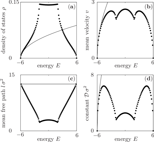
Figure 2: Energy-dependencies in the limit of weak disorder: (a) density of states, (b) mean velocity, (c) mean free path as well as (d) diffusion constant (according to the Boltzmann equation). The numerical data (circles) is extracted from a cube with $1000^{3}$ lattice sites. The known approximations for low energies (solid lines) are indicated for comparison.

Obviously, the approximations for (6) and (7) are valid for very low energies solely, i.e., in the outer tails of the density of states. The actual curves differ strongly in the details. As a consequence the curves for ${\cal D}(E)$ and $l(E)$, as displayed in figure 2 (c) and (d), show interesting features, too. Particularly, the maximum diffusion coefficient is not located at the middle of the spectrum ($E=0$). Instead two distinct maxima are observed at positions which are closer to the borders of the spectrum ($E\approx 4.5$).
The curve for ${\cal D}(E)$ seems to already indicate that the overall dynamics of all energy regimes, i.e., the dynamics at high temperatures can not be described as diffusive with a single diffusion coefficient. However, for a definite conclusion the ${\cal D}(E)$-curve has to be weighted with the density of states $\rho(E)$, of course. Therefore in figure 3 the relative number of states $r$ is shown which contribute to a certain diffusion constant.

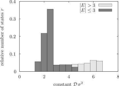
Figure 3: The relative number of states $r$ corresponding to a diffusion constant $\cal D$ (according to the Boltzmann equation), cf. Fig. 2. The bars of the histogram visualize contributions from energies $|E|>3$ (light-colored area) and from energies $|E|\leq 3$ (dark-colored area).

In a sense $r$ is again a density of states but now in the space of diffusion coefficients. Apparently, the majority of all states corresponds to diffusion constants which are rather close to ${\cal D}\approx 2.5/\sigma^{2}$, i.e., the value for $E=0$. These states are also located around the middle of the spectrum, as indicated in figure 3. But there is a relevant number of states from the outer parts of the spectrum which contribute to larger values of $\cal D$. Remarkably, in these parts the number of states with smaller values of $\cal D$ is negligible. However, figure 3 clearly demonstrates that the overall dynamics of all energy regimes is not diffusive with a single diffusion coefficient.
The situation may change, when the limit of weak disorder is slightly left, i.e., when the above predictions of the Boltzmann equation begin to break down. Obviously, the breakdown begins for the states from the borders of the spectrum, since these states are the first which become eventually localized. (The Boltzmann equation does simply not predict localization). At this point the predictions for the states from the spectral middle are still unaffected, of course. On that account it may happen that the large values of $\cal D$ in figure 3 are gradually moved towards ${\cal D}\approx 2.5/\sigma^{2}$ such that $r$ finally becomes more or less peaked at this position. In that case the dynamics is governed by a single diffusion constant. So far, this line of thoughts is a mere assumption. Even if the assumption was correct, it would be entirely unclear whether or not this assumption has some impact on a situation with strong disorder, i.e., beyond any validity of the Boltzmann equation.
In the following sections 3.2 and 3.3 we subsequently show for strong disorder that it appears to be indeed justified to describe the dynamics below the localization length as diffusive with a single diffusion coefficient. Surprisingly, this diffusion constant is rather close to the value $2.5/\sigma^{2}$, wide outside the strict validity of the Boltzmann equation.

3.2 Strong disorder: TCL projection operator technique

Our approach in the limit of strong disorder is based on the time-convolutionless (TCL) projection operator technique [17, 18] which has already been applied to the transport properties of similar models but without disorder, see [19, 20, 21]. In its standard form this approach is restricted to the infinite temperature limit. This limitation implies that energy dependencies are not resolved, i.e., our results are to be interpreted as results on an overall behavior of all energy regimes.
As illustrated in figure 4,

Figure 4: A $3$-dimensional lattice which consists of $N$ layers with $n\times n$ sites each. Only next-neighbor hoppings are taken into account. Constants for intra-layer hoppings are set to $1$ (white arrows), inter-layer hoppings are specified by another constant $\lambda$ (black arrows).

we consider a $3$-dimensional lattice consisting of $N$ layers with $n\times n$ sites each. The Hamiltonian of our model is almost identical to (1) with one single exception: All hopping terms which correspond to hoppings between layers (black arrows in figure 4) are multiplied by some constant $\lambda$. This multiplication is basically done due to technical reasons, see below. However, for $\lambda=1$ the Hamiltonian reduces to the usual Anderson Hamiltonian (1).
We now establish a coarse-grained description in terms of subunits (similarly to [22]): At first we take all those terms of the Hamiltonian which only contain the sites of the $\mu$th layer in order to form the local Hamiltonian $\hat{h}_{\mu}$ of the subunit $\mu$. Thereafter all those terms which contain the sites of adjacent layers $\mu$ and $\mu+1$ are taken in order to form the interaction $\lambda\,\hat{v}_{\mu}$ between neighboring subunits $\mu$ and $\mu+1$. Then the total Hamiltonian may be also written as

$$\hat{H}=\hat{H}_{0}+\lambda\,\hat{V}\,,\quad\hat{H}_{0}=\sum_{\mu=0}^{N-1}\hat{h}_{\mu}\,,\quad\hat{V}=\sum_{\mu=0}^{N-1}\hat{v}_{\mu}\,,$$ (9)

where we use periodic boundary conditions, e.g., we identify $\mu=N$ with $\mu=0$. The introduction of the additional parameter $\lambda$ allows for the independent adjustment of the interaction strength in this coarse-grained description. Since we are going to work in the Dirac picture, the indispensable eigenbasis of $\hat{H}_{0}$ may be found from the diagonalization of disconnected layers.
By $\hat{p}_{\mu}$ we denote the particle number operator of the $\mu$th subunit, i.e., the sum of $\hat{a}^{\dagger}_{\vec{r}}\,\hat{a}_{\vec{r}}$ over all ${\vec{r}}$ of the $\mu$th layer. Because the overall number of particles is conserved, i.e., $[\,\sum_{\mu}\hat{p}_{\mu},\hat{H}\,]=0$ and no particle-particle interactions are taken into account, we still restrict the investigation to the one-particle subspace. The actual state of the system is naturally represented by a time-dependent density matrix $\rho(t)$, i.e., the quantity $p_{\mu}(t)=\textnormal{Tr}\{\,\rho(t)\,\hat{p}_{\mu}\,\}$ is the probability for locating the particle somewhere within the $\mu$th subunit. The consideration of these coarse-grained probabilities corresponds to the analysis of transport along the direction which is perpendicular to the layers. Instead of simply characterizing whether or not there is transport at all, we analyze the full dynamics of the $p_{\mu}(t)$.
The dynamical behavior of the $p_{\mu}(t)$ may be called diffusive, if the $p_{\mu}(t)$ fulfill a discrete diffusion equation

$$\dot{p}_{\mu}(t)={\cal D}\,[\,p_{\mu-1}(t)-2\,p_{\mu}(t)+p_{\mu+1}(t)\,]$$ (10)

with some $\mu$- and $t$-independent diffusion constant $\cal D$. It is a straightforward manner to show (multiplying (10) by $\mu$, respectively $\mu^{2}$, performing a sum over $\mu$ and manipulating indices on the r.h.s.) that the spatial variance

$$\textnormal{Var}(t)=\sum_{\mu=0}^{N-1}\mu^{2}\,p_{\mu}(t)-\left[\,\sum_{\mu=0}^{N-1}\mu\,p_{\mu}(t)\,\right]^{2}$$ (11)

increases linearly with $t$, i.e., $\textnormal{Var}(t)=2\,{\cal D}\,t$. Contrary, ballistic behavior is characterized by $\textnormal{Var}(t)\propto t^{2}$, while insulating behavior corresponds to $\textnormal{Var}(t)=\textnormal{const.}$, of course.
According to Fourier’s work, diffusions equations are routinely decoupled with respect to, e.g., cosine-shaped spatial density profiles

$$p_{q}(t)=C_{q}\sum_{\mu=0}^{N-1}\cos(q\,\mu)\,p_{\mu}(t)\,,\quad q=\frac{2\pi\,k}{N}\,,\quad k=0,1,\ldots,\frac{N}{2}$$ (12)

and a yet arbitrary normalization constant $C_{q}$. Consequently, (10) yields

$$\dot{p}_{q}(t)=-2\,(1-\cos q)\,{\cal D}\,p_{q}(t)\,.$$ (13)

Therefore, if the quantum model indeed shows diffusive transport, all modes $p_{q}(t)$ have to relax exponentially. If, however, the modes $p_{q}(t)$ are found to relax exponentially only for some regime of $q$, the model is said to behave diffusively on the corresponding length scale $l=\pi/q$. One might think of a length scale which is both large compared to the mean free path (below that ballistic behavior occurs, $\sigma^{2}(t)\propto t^{2}$) and small compared the localization length (beyond that insulating behavior appears, $\sigma^{2}(t)=\textnormal{const.}$).
For our purposes, i.e., for the application of the TCL projection operator technique, it is convenient to express the modes $p_{q}(t)$ as the expectation values of respective mode operators $\hat{p}_{q}$, namely,

$$p_{q}(t)=\textnormal{Tr}\{\,\rho(t)\,\hat{p}_{q}\,\}\,,\quad\hat{p}_{q}=C_{q}\sum_{\mu=0}^{N-1}\cos(q\,\mu)\,\hat{p}_{\mu}\,,$$ (14)

where the normalization constants $C_{q}$ are now chosen such that $\textnormal{Tr}\{\,\hat{p}_{q}^{2}\,\}=1$. With this normalization

$${\cal P}\,\rho(t)=\textnormal{Tr}\{\,\rho(t)\,\hat{p}_{q}\,\}\,\hat{p}_{q}=p_{q}(t)\,\hat{p}_{q}\,$$ (15)

defines a suitable projection (super)operator, because ${\cal P}^{2}={\cal P}$. For those initial states $\rho(0)$ which satisfy ${\cal P}\,\rho(0)=\rho(0)$, i.e., for harmonic density profiles the TCL projection operator technique eventually leads to a differential equation of the form

$$\dot{p}_{q}(t)=R_{q}(t)\,p_{q}(t)\,,\quad R_{q}(t)=\lambda^{2}\,R_{2,q}(t)+\lambda^{4}\,R_{4,q}(t)+\ldots$$ (16)

which is a formally exact description for the dynamics at high temperatures, since $\rho(0)$ is not restricted to any energy subspaces. Apparently, the dynamics of $p_{q}(t)$ is controlled by a time-dependent decay rate $R_{q}(t)$. This decay rate is given in terms of a systematic perturbation expansion in powers of the inter-layer coupling. (Concretely, for this model all odd orders vanish.) At first we concentrate on the truncation of (16) to lowest order, i.e., to second order. But the fourth order is considered afterwards in order to estimate the validity of this second order truncation.
According to [18], the TCL formalism routinely yields the second order prediction

$$\dot{p}_{q}(t)=\lambda^{2}\,R_{2,q}(t)\,p_{q}(t)\,,\quad R_{2,q}(t)=\int_{0}^{t}\textnormal{d}\Delta\,f_{q}(\Delta)$$ (17)

with the two-point correlation function

$$f_{q}(\Delta)=\textnormal{Tr}\Big{\{}[\,\hat{V}(t),\hat{p}_{q}\,]\,[\,\hat{V}(t^{\prime}),\hat{p}_{q}\,]\Big{\}}\,,\quad\Delta=t-t^{\prime}\,,$$ (18)

where the time dependencies of operators are to be understood with respect to the Dirac picture. The $q$-dependence in (18) is significantly simplified under the following assumption: The autocorrelation functions $\textnormal{Tr}\{\,\hat{v}_{\mu}(t)\,\hat{v}_{\mu}(t^{\prime})\,\}$ of the local interactions $\hat{v}_{\mu}$ should depend only negligibly on the layer number $\mu$ (at relevant time scales). In fact, numerics indicate that this assumption is well fulfilled (for the values of $\sigma$ which are discussed here), once the layer sizes exceed ca. $30\times 30$. Therefore first investigations may be based on the consideration of an arbitrarily chosen junction of two layers. The local interaction between these representative layers may be called $\hat{v}_{0}$. The use of the above assumption simplifies (18) to

$$f_{q}(\Delta)\approx-2\,(1-\cos q)\,f(\Delta)\,,\quad f(\Delta)=\frac{1}{n^{2}}\,\textnormal{Tr}\{\,\hat{v}_{0}(t)\,\hat{v}_{0}(t^{\prime})\,\}\,,$$ (19)

where the $q$-dependence enters solely as an overall scaling factor [21]. As a consequence the second order prediction at high temperatures reads

$$\dot{p}_{q}(t)\approx-2\,(1-\cos q)\,\lambda^{2}\,R_{2}(t)\,p_{q}(t)\,,\quad R_{2}(t)=\int_{0}^{t}\textnormal{d}\Delta\,f(\Delta)\,.$$ (20)

This equation is already very similar to (13) but still contains a time-dependent diffusion coefficient ${\cal D}(t)=\lambda^{2}\,R_{2}(t)$. However, it numerically turns out that $f(\Delta)$ behaves like a standard correlation function, i.e., it decays completely within some time scale $\tau_{C}$. After this correlation time $f(\Delta)$ approximately remains zero and $R_{2}(t)$ takes on a constant value $R_{2}$, the area under the initial peak of $f(\Delta)$. Numerics indicates that neither $\tau_{C}$ nor $R_{2}$ depend substantially on $n$ (at least for $n>30$) such that both $\tau_{C}$ and $R_{2}$ are essentially functions of $\sigma$. Since the correlation time $\tau_{C}$ apparently is independent from $q$ and $\lambda$, it is always possible to realize a relaxation time

$$\tau_{R}=\frac{1}{2\,(1-\cos q)\lambda^{2}R_{2}}$$ (21)

which is much larger than $\tau_{C}$, e.g., in an infinitely large system there definitely is a small enough $q$. For $\tau_{R}\gg\tau_{C}$ the second order prediction (20) at high temperatures immediately becomes

$$\dot{p}_{q}(t)\approx-2\,(1-\cos q)\,\lambda^{2}\,R_{2}\,p_{q}(t)$$ (22)

and the comparison with (13) clearly shows diffusive behavior with a diffusion constant ${\cal D}=\lambda^{2}\,R_{2}$. Due to the independence of $R_{2}$ from $n$ (again for $n>30$) the pertinent diffusion constant for arbitrarily large systems may be quantitatively inferred from a finite, e.g., $30\times 30$ layer, see figure 5.

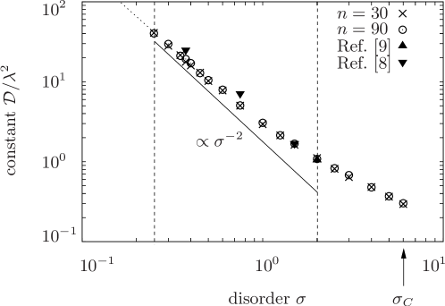
Figure 5: Theoretical prediction of lowest order TCL for an energy-independent diffusion constant $\cal D$ as a function of the disorder $\sigma$ (Gaussian distribution) for the layer sizes $n=30$ (crosses) and $n=90$ (circles). The theoretical prediction is shown up to the critical disorder $\sigma_{C}\approx 6$ and the validity range of this prediction is displayed (dashed lines). As a guide for the eyes a proportionality to $\sigma^{-2}$ is indicated (solid line). For comparison the value ${\cal D}=1.05\pm 0.10$ from [9] is shown (triangle), as found therein for $E=0$ and $\sigma=2$ (Gaussian distribution). Further values for $\cal D$ from [8] are displayed (triangles), as obtained therein for $E=0$ but for $W=1$, $2$ and $4$ (box distribution). In that case data for Gaussian and box distributions are supposed to be simply convertible by $W/\sigma\approx 2.6$ (according to the ratio of the critical values). The prediction for $E=0$ according to the Boltzmann equation is also indicated (dotted line).

Therein $\cal D$ is evaluated for the range of $\sigma$ where the used approximation for the $q$-dependence of the correlation function turns out to be justified, cf. (18) and (19). We additionally indicate already the validity range of the second order prediction at high temperatures, although this point is firstly discussed in detail in the next section 3.3. However, within the validity range there indeed is a corridor of $q$ in which the dynamics at high temperatures can be described as diffusive in terms of (22). Outside the validity range such a $q$-corridor does not exist, since either diffusion constants become highly energy dependent ($\sigma<0.2$) or localized contributions become non-negligible ($\sigma>2$), cf. figure 1.
As indicated in figure 5, at the l.h.s. of the validity range the diffusion coefficient simply scales as ${\cal D}\propto 1/\sigma^{2}$. Because such a scaling is expected in the limit of weak disorder, we quantitatively compare with the result $2.5/\sigma^{2}$ for $E=0$ ($\lambda=1$) according to the Boltzmann equation, although the weak disorder limit is reached by no means, even for the energy regime around $E=0$. The surprisingly good agreement supports the line of thoughts in section 3.1, namely, the diffusion constants at all energies are rather close to the value $2.5/\sigma^{2}$, when the disorder becomes non-weak. At the r.h.s. of the validity range the diffusion coefficient begins to deviate from a simple $1/\sigma^{2}$-scaling, e.g., ${\cal D}\approx 1.05\,\lambda^{2}$ for $\sigma=2$. This value excellently agrees with the one in [9] which is found therein by a numerical study of Green’s functions. The study in [9] remarkably requires an ensemble average over very many realizations of disorder, while a single disorder realization is adequate here, i.e., the correlation function is a self-averaging object.
So far, we have characterized the diffusive regime. We now turn towards an investigation of the ballistic regime.

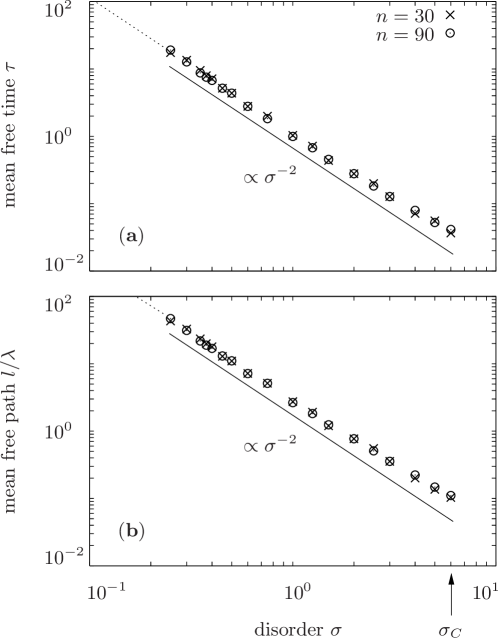
Figure 6: Theoretical prediction of lowest order TCL for an energy-independent (a) mean free time $\tau$ and (b) mean free path $l$ w.r.t. the disorder $\sigma$ (Gaussian distribution) for the layer sizes $n=30$ (crosses) as well as $n=90$ (circles). As a guide for the eyes proportionalities to $\sigma^{-2}$ are shown (solid lines). The predictions for $E=0$ according to the Boltzmann equation are also shown (dotted lines). The results in (a) and (b) suggest a mean velocity $v/\lambda\approx 2.5$.

Obviously, the replacement of (20) by (22) is only self-consistent for $\tau_{R}\gg\tau_{C}$, i.e., if the relaxation time is much larger than the correlation time. But this criterion has to break down for sufficiently large $q$, see figure 1. Hence, a transition from the diffusive to the ballistic regime appears for those modes $p_{q}(t)$ which decay on an intermediate time scale $\tau_{R}\approx\tau_{C}$, while the ballistic regime is finally reached for those modes $p_{q}(t)$ which decay on a short time scale $\tau_{R}\ll\tau_{C}$. In fact, the rate $R_{2}(t)$ is found to increase linearly for $t<\tau_{C}/2\pi$. Due to this linear increase the second order prediction at high temperatures is a Gaussian decay of the corresponding modes. Such a Gaussian decay is known to be typical for ballistic dynamics [19, 20, 21]. However, the ballistic character of the dynamics is most convincingly demonstrated in terms of the variance $\textnormal{Var}(t)$, as defined in (11). The second order prediction at high temperatures for this variance is given by

$$\textnormal{Var}_{2}(t)=2\,\lambda^{2}\int_{0}^{t}\textnormal{d}t^{\prime}\,R_{2}(t^{\prime})$$ (23)

and scales as $\textnormal{Var}_{2}(t)\propto t^{2}$ for $t<\tau_{C}/2\pi$. Of course, this result suggests the mean free time $\tau=\tau_{C}/2\pi$. Consequently, in order to obtain the mean free path as well, a mode $p_{q}(t)$ with $\tau_{R}=\tau$ has to be considered, i.e., the condition $p_{q}(\tau)/p_{q}(0)=1/e$ has to be fulfilled. This condition and (20) yield

$$2\,(1-\cos q)\,\lambda^{2}\,\int_{0}^{\tau}\textnormal{d}t^{\prime}\,R_{2}(t^{\prime})=1$$ (24)

which can be rewritten as $(1-\cos q)\,\textnormal{Var}_{2}(\tau)=1$. The use of $l=\pi/q$ eventually leads to the expression for the mean free path

$$l=\frac{\pi}{\arccos[1-1/\textnormal{Var}_{2}(\tau)]}$$ (25)

or the approximation $l\approx\pi/\sqrt{2}\,\sqrt{\textnormal{Var}_{2}(\tau)}$ for $l\gg 1$, i.e., about two times the standard deviation. We use this approximation, because the dependence on $\lambda$ becomes trivial, namely, $l\propto\lambda$. However, whenever $l\approx 1$ or even smaller, the concrete value of the mean free path is less important, since then the ballistic regime is restricted to a length scale below a single lattice site and does simply not exist.
As indicated in figure 6, both the mean free time $\tau$ and the mean free path $l$ are proportional to $1/\sigma^{2}$ over the full range of accessible $\sigma$ where the used approximation for the $q$-dependence of the correlation function turns out to be justified, cf. (18) and (19). Therefore the mean velocity $v=l/\tau$ becomes independent from $\sigma$. Again there is a quantitative agreement with the prediction for $E=0$ ($\lambda=1$) according to the Boltzmann equation, wide outside the weak disorder limit. In contrast to figure 5, the validity range of the second order prediction at high temperatures is not indicated in figure 6, since this prediction for short times is expected to be valid for all accessible $\sigma$, see the next section 3.3. However, for $\sigma>1.5$ the mean free path $l$ takes on values which are smaller than $\lambda$, e.g., for $\lambda=1$ the ballistic regime is practically absent.

3.3 Validity range of the TCL-based theory

In the present section we are going to discuss the validity range of the second order prediction at high temperatures in more detail. To this end we consider the ratio ${\cal R}(t)$ of the fourth order to the second order, namely,

$${\cal R}(t)=\frac{\lambda^{4}\,R_{4,q}(t)}{2\,\lambda^{2}\,(1-\cos q)\,R_{2}(t)}\,,$$ (26)

cf. (16). Whenever ${\cal R}(t)\ll 1$, the second order term $2\,\lambda^{2}\,(1-\cos q)\,R_{2,q}(t)$ dominates the decay of the modes $p_{q}(t)$ and the fourth order term $\lambda^{4}\,R_{4,q}(t)$ is negligible. But in general already the direct evaluation of the fourth order term turns out be extremely difficult, both analytically and numerically. However, by the use of the techniques in [21, 23, 24] the fourth order term can be approximated by

$$\lambda^{4}\,R_{4,q}(t)\approx 4\,\lambda^{4}\,(1-\cos q)^{2}\,R_{4}(t)$$ (27)

with the remaining $q$-independent rate

$$R_{4}(t)=t\,\left[\frac{1}{n^{2}}\sum_{i}\left(\int_{0}^{t}\textnormal{d}\Delta\,\langle\psi_{i}|\,\hat{v}_{0}(t)\,\hat{v}_{0}(t^{\prime})\,|\psi_{i}\rangle\right)^{2}-R_{2}(t)^{2}\right]\,,$$ (28)

where $|\psi_{i}\rangle$ denote the eigenstates of $\hat{H}_{0}$. Consequently, in complete analogy to the rate $R_{2}(t)$, also the rate $R_{4}(t)$ may be evaluated from the consideration of an arbitrarily chosen junction of two layers. The local interaction between these representative layers is still called $\hat{v}_{0}$. The above approximation is based on the fact that the interaction $\hat{V}$ features the so-called Van Hove structure [25, 26], i.e., $\hat{V}^{2}$ essentially is a diagonal matrix (in the eigenbasis of $\hat{H}_{0}$). However, for the concrete derivation of this approximation we refer to [21] and concentrate on the implications here. By the use of the approximation the ratio ${\cal R}(t)$ can be rewritten as

$${\cal R}(t)\approx{\cal Q}\,\frac{R_{4}(t)}{R_{2}(t)}\,,\quad{\cal Q}=2\,\lambda^{2}\,(1-\cos q)\,.$$ (29)

This ratio is a monotonically increasing function of $t$, cf. (28). As a consequence there always exists a time $t_{B}$ with ${\cal R}(t_{B})=1$, i.e., a time where the contributions $R_{2}(t)$ and $R_{4}(t)$ are equally large. But this fact does not restrict the validity of the second order prediction, if $t_{B}\gg\tau_{R}$ and hence ${\cal R}(\tau_{R})\ll 1$. The validity obviously breaks down only in the case of, say, ${\cal R}(\tau_{R})\approx 1$ or even larger. Since both ${\cal R}(t)$ and $\tau_{R}$ depend on $\cal Q$, we use again the condition $p_{q}(\tau_{R})/p_{q}(0)=1/e$, i.e.,

$${\cal Q}\int_{0}^{\tau_{R}}\textnormal{d}t^{\prime}\,R_{2}(t^{\prime})=1$$ (30)

in order to replace $\cal Q$ in (29). Due to this replacement ${\cal R}(\tau_{R})$ becomes a function

$${\cal R}(\tau_{R})=\frac{R_{4}(\tau_{R})}{R_{2}(\tau_{R})\,\int_{0}^{\tau_{R}}\textnormal{d}t^{\prime}\,R_{2}(t^{\prime})}$$ (31)

of the free variable $\tau_{R}$. ($\tau_{R}$ still depends on $\cal Q$, of course.) Because also ${\cal R}(\tau_{R})$ increases monotonically, we define $\textnormal{max}(\tau_{R})$ as the maximum $\tau_{R}$ for which ${\cal R}(\tau_{R})$ is still smaller than $1$. This maximum relaxation time already specifies the validity range of the second order prediction. However, it is useful to set $\textnormal{max}(\tau_{R})$ in relation to the correlation time $\tau_{C}$.

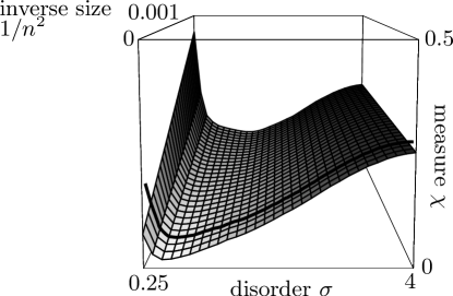
Figure 7: The measure $\chi$ for the validity range of lowest order TCL as a function of the disorder $\sigma$ and the inverse layer size $1/n^{2}$. This measure detects the “corridor” of wave numbers, where transport is diffusive at almost all energies with a single diffusion constant, cf. Fig. 1. For those values of $\chi$ which are on the order of $1/4$ the corridor does not exist. But for those values of $\chi$ which are closer to zero the corridor opens. The smaller $\chi$, the larger is this corridor. An absolute minimum $\chi_{\textnormal{min}}\approx 1/50$ is found at $\sigma\approx 1/2$ in the limit $n\rightarrow\infty$. Note that only $10\%$ of the whole area is extrapolated (the area in front of the thick line).

We therefore define the measure $\chi$ as the dimensionless quantity $\chi=\tau_{C}/\textnormal{max}(\tau_{R})$, e.g., $\chi=1$ directly implies the breakdown of the second order prediction on relatively short time scales on the order of $\tau_{C}$, whereas $\chi=0$ strongly indicates its unrestricted validity. For practical purposes an interpretation of $\chi$ in the context of length scales certainly is advantageous. Such an interpretation essentially requires the inversion of (30). In general this inversion can only be done by numerics. But we have $\tau_{R}=1/({\cal Q}R_{2})$ for $\tau_{R}\gg\tau_{C}$ and may hence write

$$\frac{1}{{\cal Q}_{\textnormal{max}}\,R_{2}}=2\,\tau_{C}\,,\quad\frac{1}{{\cal Q}_{\textnormal{min}}\,R_{2}}=\frac{\textnormal{max}(\tau_{R})}{2}\,,$$ (32)

where the factors $2$ and $1/2$ are chosen to slightly fulfill $\tau_{C}\ll\tau_{R}\ll\textnormal{max}(\tau_{R})$, i.e., ${\cal Q}_{\textnormal{max}}$, ${\cal Q}_{\textnormal{min}}$ correspond to lower, respectively upper border of the diffusive corridor, cf. figure 1. We finally end up with

$$\frac{{\cal Q}_{\textnormal{min}}}{{\cal Q}_{\textnormal{max}}}=4\chi$$ (33)

or by the use of ${\cal Q}\approx q^{2}\,\lambda^{2}$ with $q_{\textnormal{min}}/q_{\textnormal{max}}\approx 2\sqrt{\chi}$. Thus, for those values of $\chi$ which are on the order of $1/4$ the corridor does not exist. But for those values of $\chi$ which are closer to zero the corridor opens. The smaller $\chi$, the larger is this corridor.
In figure 7 the measure $\chi$ is quantitatively evaluated as a function of the amount of disorder $\sigma$ and the inverse layer size $1/n^{2}$. (The rate $R_{4}(t)$, other than the rate $R_{2}(t)$, scales significantly with $n$. This scaling gives rise to the $n$-dependence of $\chi$.) For each layer size there is a optimum disorder where $\chi$ is minimized, i.e., where the diffusive corridor is maximized. But for $n=30$ (back of figure 7) we find $2\sqrt{\chi}\approx 2/3$ at the optimum disorder. This value indicates a corridor of about one or two diffusive modes (for $N=30$). For all $\sigma$ and $n\leq 100$ (which is the limit for our numerics) $\chi$ clearly appears to be of the form

$$\chi(\sigma,n)=\frac{A(\sigma)}{n^{2}}+B(\sigma)\,.$$ (34)

The extrapolation of the $1/n^{2}$-scaling eventually leads to a suggestion for $n=\infty$ (front of figure 7). According to this suggestion, we find $2\sqrt{\chi}\approx 2/7$, again at the optimum disorder. This value indicates a still narrow but existent corridor of diffusive modes (for N = $\infty$).
We finally recall that these findings apply at infinite temperature, i.e., the narrow diffusive corridor is characterized by the fact that the dynamics within this corridor is diffusive at almost all energies with a single diffusion coefficient. The narrowness of this corridor passes into a complete absence, since either diffusion constants become highly energy dependent ($\sigma<0.2$) or localized contributions become non-negligible ($\sigma>2$), cf. figure 1.

3.4 Numerical verification

In the last two sections we have introduced the TCL-based method and have discussed its predictions as well as the validity of these predictions. In the present section we are going to present the results of numerical simulations in order to verify the predictions of the method, as far as possible from the consideration of a finite system. Since the applicability of the method requires a system which consists of layers with a minimum size of $n=30$, we consider layers of that size in the following simulations. According to the predictions of the method, for $n=30$ a diffusive corridor is only existent for disorders in the vicinity of $\sigma=1$, see figure 7. Therefore we focus on such a value of $\sigma$ in all numerical simulations.
For $\sigma=1$ the TCL-based theory predicts a diffusion constant ${\cal D}\approx 2.9\,\lambda^{2}$ and a mean free time $\tau\approx 1.1$, i.e., a correlation time $\tau_{C}=2\pi\,\tau\approx 6.9$, cf. figures 5 and 6.

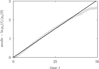
Figure 8: Results for the time evolution of a mode $p_{q}(t)$ with $q=\pi/20$ (without any restriction to energy regimes). The numerical data (circles) is obtained by the use of a $4$th order Suzuki-Trotter integrator for the model parameters $N=40$, $n=30$, $\sigma=1$ (Gaussian distribution) and $\lambda=1$ (isotropic hopping constants). The theoretical prediction of lowest order TCL (solid line) is indicated for comparison.

According to the theory, diffusive dynamics emerges only on a time scale which is given by the condition $\tau_{C}\ll\tau_{R}=1/[2\,(1-\cos q)\,{\cal D}]$, e.g., a sufficiently small $q$ has to be chosen. For the naturally interesting isotropic case of $\lambda=1$ the choice $q=\pi/20$ leads to the ratio $\tau_{R}/\tau_{C}\approx 2.0$. Unfortunately, $q=\pi/20$ is firstly realized for a system which consists of $N=40$ layers and such a system already is too large for the application of numerically exact diagonalization.
However, approximative numerical integrators may be applied, e.g., on the basis of a Suzuki-Trotter decomposition of the time evolution operator [27, 28, 29]. In detail we choose a pure initial state $|\psi_{q}(0)\rangle$ and apply a fourth order Suzuki-Trotter integrator in order to obtain the time evolution $|\psi_{q}(t)\rangle$ of this initial state and to evaluate the actual expectation value $p_{q}(t)=\langle\psi_{q}(t)|\,\hat{p}_{q}\,|\psi_{q}(t)\rangle$. In particular we choose the initial state at random and only require the condition $\langle\psi_{q}(0)|\,\hat{p}_{q^{\prime}}\,|\psi_{q}(0)\rangle=\delta_{q,q^{\prime}}$, i.e., we still consider a harmonic density profile. The result of the approximative numerical integrator is shown in figure 8 for a single realization of $|\psi_{q}(0)\rangle$ with $q=\pi/20$. Apparently, there is a very good agreement between this result and the prediction of the TCL-based theory. The latter agreement further demonstrates that the validity of the theoretical prediction is not restricted to an initial density matrix of the strict form $\rho(0)=\hat{p}_{q}$. This fact may be understood in terms of dynamical typicality [30, 31, 32, 33, 34].
Although the above Suzuki-Trotter integrator allows to determine the time evolution of pure initial states for rather large systems, this integrator is not able to resolve the energy dependencies of the dynamics, of course. To this end we have to use numerically exact diagonalization which is applicable to a maximum system with about $N=10$ layers.

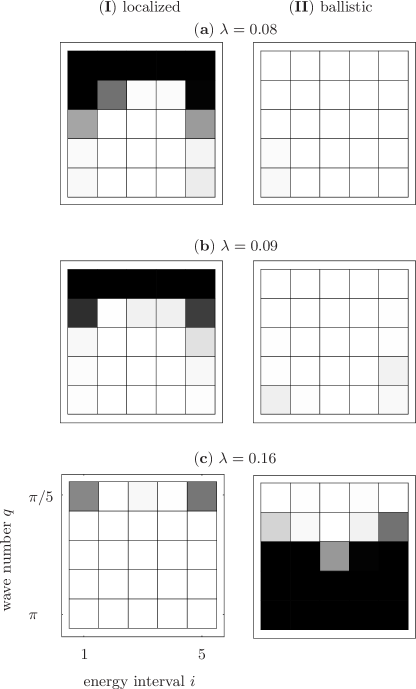
Figure 9: Numerical results for the deviation of transport from diffusive towards (I) localized and (II) ballistic behavior as a function of the wave number $q$ and the energy interval $i$ for inter-layer hopping constants (a) $\lambda=0.08$, (b) $\lambda=0.09$ and (c) $\lambda=0.16$. The color palette is chosen from white (small deviations) to black (large deviations). The underlying data is obtained from exact diagonalization for the model parameters $N=10$, $n=30$ and $\sigma=1$ (Gaussian distribution).

In such a system diffusive dynamics is expected to emerge only, if the coupling constant $\lambda$ is much decreased. For $\lambda\ll 1$, in complete analogy to the above numerical simulation, the time evolution of pure initial states has comprehensively been shown to be in full accord with all predictions of the TCL-based theory [24, 21]. However, since it still remains to resolve the energy dependencies of the dynamics, we consider the quantities

$$p_{q,E}(t)=\textnormal{Tr}\{{\cal P}_{E}\,\rho(t)\,{\cal P}_{E}\,\hat{p}_{q}\}\,,$$ (35)

where ${\cal P}_{E}$ denotes a projector onto the states of some energy regime $E$. In pratice we choose a coarse-grained partition into five energy intervals with the same number of states, namely, there are $1800$ states in each energy interval. A fine-grained partition into more energy intervals is not convenient, because only a sufficiently coarse-grained partition assures $p_{q}(t)\approx\sum_{E}p_{q,E}(t)$, i.e, the quantities $p_{q,E}(t)$ resolve the dynamics on a reasonable energy scale. (The longer the relevant time scale for the dynamics, the smaller is this reasonable energy scale, of course.)
The quantities $p_{q,E}(t)$ can be used in order to provide a diagram for the dependence of transport on $q$ and $E$, similar to the sketch in figure 1. For instance, two measures for the deviation of $p_{q,E}(t)$ from a strictly exponential decay (diffusive behavior) may be defined, cf. [35]: The first measure detects deviations towards a Gaussian decay at short times (ballistic behavior) and the second measure detects deviations towards a stagnant decay at long times (localized behavior). Such measures are displayed in figure 9. Whenever one of these measures is large (black areas), $p_{q,E}(t)$ does not relax exponentially. But whenever both measures are small (white areas), $p_{q,E}(t)$ decays exponentially, i.e., it behaves diffusively. Particularly, there indeed is a $q$-corridor where $p_{q,E}(t)$ decays exponentially for practically all $E$. As predicted by the TCL-based theory, this diffusive corridor is shifted to smaller $q$, when $\lambda$ is increased. According to figure 9 (c), the borders $q_{\textnormal{min}}$, $q_{\textnormal{max}}$ of the diffusive corridor lead to a ratio $q_{\textnormal{min}}/q_{\textnormal{max}}$ between $1/2$ and $1$. The latter ratio remarkably is in accord with the theoretical prediction $q_{\textnormal{min}}/q_{\textnormal{max}}\approx 2/3$, too. (In general the ratio ${\cal Q}_{\textnormal{min}}/{\cal Q}_{\textnormal{max}}$ has to be compared. But for the borders in figure 9 (c) the approximation ${\cal Q}\approx\lambda^{2}\,q^{2}$ is already justified.)
However, it still remains to clarify whether or not the dynamics within the diffusive corridor is governed by a single diffusion coefficient.

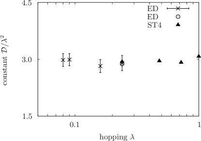
Figure 10: Results for the diffusion coefficient $\cal D$ as a function of the inter-layer hopping constant $\lambda$ for the model parameters $n=30$ and $\sigma=1$ (Gaussian distribution). The data corresponding to figure 9 is indicated by crosses (mean value of energy intervals) with bars (mean deviation of energy intervals). Additional data without any restriction to energy regimes is presented for $N=10$ from exact diagonalization (circle) and for $N=10$, $20$, $30$, $40$ by the use of a $4$th order Suzuki-Trotter integrator (triangles), cf. figure 8.

To this end an exponential fit may be applied to $p_{q,E}(t)$ for each $E$ in this $q$-corridor. Such a fit directly yields a decay rate and consequently a diffusion coefficient ${\cal D}_{E}$. Then the mean value ${\cal D}$ and the mean deviation $\delta{\cal D}$ of the energy intervals may be evaluated, see figure 10. For all $\lambda$ where a diffusive corridor exists for $N=10$ we find a mean value ${\cal D}$ between $2.9\,\lambda^{2}$ and $3.0\,\lambda^{2}$ and a mean deviation $\delta{\cal D}$ on the order of less than $10\%$. This finding finally supports the theoretical prediction for a diffusive corridor with a single diffusion coefficient. For completeness, figure 10 additionally shows diffusion coefficients from a exponential fit to $p_{q}(t)$, as obtained by the use of the above Suzuki-Trotter integrator for pure initial states. Even though $\delta{\cal D}$ is not availabe in that case, $\cal D$ scales simply as ${\cal D}\propto\lambda^{2}$ for all $\lambda$ up to the isotropic case of $\lambda=1$.

4 Summary and conclusion

In the work at hand we have investigated single-particle transport in the $3$-dimensional Anderson model with Gaussian on-site disorder. Particularly, our investigation has been focused on the dynamics on scales below the localization length. The dynamics on those scales has been analyzed with respect to its dependence on the amount of disorder and the energy interval. This analysis has especially included the quantitative evaluation of the characteristic transport quantities, e.g., the mean free path which separates ballistic and diffusive transport regimes. For these regimes mean velocities, respectively diffusion coefficients have been evaluated quantitatively, too.
By the use of the Boltzmann equation in the limit of weak disorder we have shown that all transport quantities substantially depend on the energy interval. In addition we have demonstrated that these energy dependencies significantly differ from the well known approximations for a free electron gas. This significant difference develops for energies around the spectral middle where the overwhelming majority of all states is located. As a consequence the diffusion coefficients for these energies seem to be both a new and relevant result.
In the limit of strong disorder we have found evidence for much less pronounced energy dependencies by an application of a method on the basis of the TCL projection operator technique. This method suggests that all transport quantities take on values which are practically independent from the energy interval. Remarkably, the latter values coincide with the prediction of the Boltzmann equation for the spectral middle, if this prediction is simply extrapolated to strong disorders, i.e., to disorders beyond any strict validity of the Boltzmann equation. Solely the suggested diffusion coefficient begins to differ from such a simple extrapolation, once the amount of disorder becomes on the order of the critical disorder. In the strict sense the TCL-based method does not yield a diffusion constant in the close vicinity of the critical disorder, because the validity range of the method is left for such an amount of disorder. In the close vicinity of the critical disorder the diffusion constant has to be understood as a mere conjecture. However, the method leads to a reliable diffusion coefficient for strong disorders which pass through almost one order of magnitude. Such a comprehensive description appears to be novel in the literature.
Strictly speaking, the TCL-based theory makes only a definite conclusion on a corridor of finite length scales where the dynamics is diffusive at approximately all energies with a single diffusion coefficient. But we do not expect that the diffusion coefficient in the diffusive regime outside this corridor is significantly different, especially since diffusion constants should not depend on the length scale per definition. The latter expectation is also supported by the agreement with the Boltzmann equation and with the numerical results for diffusion constants in [8, 9]. However, whenever the above corridor of length scales is not existent, the theory does not allow for any conclusion. Since such a corridor may not exist in lower dimensions, the TCL-based theory may not lead to results on transport in the one- or two-dimensional Anderson model. But the theory itself, as demonstrated for the three-dimensional case, can analogously be applied also to the lower-dimensional cases, of course. This application is a scheduled project for the near future.

References

References

- [1] Anderson P W 1958 Phys. Rev. 109 1492
- [2] Kramer B and MacKinnon A 1993 Rep. Progr. Phys. 56 1469
- [3] Grussbach H and Schreiber M 1995 Phys. Rev. B 51 663
- [4] Slevin K and Ohtsuki T 1999 Phys. Rev. Lett. 82 382
- [5] Lee P A and Ramakrishnan T V 1985 Rev. Mod. Phys. 57 287
- [6] Abou-Chacra R, Thouless D J and Anderson P W 1973 J. Phys. C 6 1734
- [7] Abrahams E, Anderson P W, Licciardello D C and Ramakrishnan T V 1979 Phys. Rev. Lett. 42 673
- [8] Markoš P 2006 Preprint arXiv:cond-mat/0609580
- [9] Brndiar J and Markoš P 2008 Preprint arXiv:0801.1610
- [10] Lherbier A, Biel B, Niquet Y-M and Roche S 2008 Phys. Rev. Lett. 100 036803
- [11] Dunlap D H, Wu H-L, and Phillips P W 1990 Phys. Rev. Lett. 65 88
- [12] Bellani V, Diez E, Hey R, Toni L, Tarricone L, Parravicini G B, Domínguez-Adame F, and Gómez-Alcalá R 1999 Phys. Rev. Lett. 82 2159
- [13] Peierls R E 1965 Quantum Theory of Solids (Oxford University Press)
- [14] Kadanoff L P and Baym G 1962 Quantum Statistical Mechanics (Benjamin)
- [15] Cercignani C 1988 The Boltzmann Equation and Its Applications (Springer)
- [16] Bartsch C, Steinigeweg R and Gemmer J 2010 Phys. Rev. E to be published (Preprint arXiv:1004.5364)
- [17] Chaturvedi S and Shibata F 1979 Z. Phys. B 35 297
- [18] Breuer H-P and Petruccione F 2007 The Theory of Open Quantum Systems (Oxford University Press)
- [19] Steinigeweg R, Breuer H-P and Gemmer J 2007 Phys. Rev. Lett. 99 150601
- [20] Michel M, Steinigeweg R and Weimer H 2007 Eur. Phys. J. Special Topics 151 13
- [21] Steinigeweg R, Gemmer J, Breuer H-P and Schmidt H-J 2009 Eur. Phys. J. B 69 275
- [22] Weaver R 2006 Phys. Rev. E 73 036610
- [23] Bartsch C, Steinigeweg R and Gemmer J 2008 Phys. Rev. E 77 011119
- [24] Steinigeweg R and Gemmer J 2010 Physica E 42 572
- [25] Van Hove L 1954 Physica 21 517
- [26] Van Hove L 1957 Physica 23 441
- [27] Trotter H F 1959 Proc. Am. Math. Soc. 10 545
- [28] Suzuki M 1990 Phys. Lett. A 146 319
- [29] Steinigeweg R and Schmidt H-J 2006 Comp. Phys. Comm. 174 853
- [30] Goldstein S, Lebowitz J L, Tumulka R and Zanghi N 2006 Phys. Rev. Lett. 96 050403
- [31] Popescu S, Short A J and Winter A 2006 Nature Phys. 2 754
- [32] Reimann P 2007 Phys. Rev. Lett. 99 160404
- [33] Bartsch C and Gemmer J 2009 Phys. Rev. Lett. 102 110403
- [34] Gemmer J, Michel M and Mahler G 2010 Quantum Thermodynamics: Emergence of Thermodynamic Behavior Within Composite Quantum Systems (Springer)
- [35] Steinigeweg R, Gemmer J and Michel M. 2006 Europhys. Lett. 75 406