Rate-Constrained Simulation
and Source Coding IID Sources

Abstract

Necessary conditions for asymptotically optimal sliding-block or stationary codes for source coding and rate-constrained simulation of memoryless sources are presented and used to motivate a design technique for trellis-encoded source coding and rate-constrained simulation. The code structure has intuitive similarities to classic random coding arguments as well as to “fake process” methods and alphabet-constrained methods. Experimental evidence shows that the approach provides comparable or superior performance in comparison with previously published methods on common examples, sometimes by significant margins.

I Introduction

The basic goal of Shannon source coding with a fidelity criterion or lossy data compression is to covert an information source $\{X_{n}\}$ into bits which can be decoded into a good reproduction of the original source, ideally the best possible reproduction with respect to a fidelity criterion given a constraint on the rate of transmitted bits. Memoryless discrete-time sources have long been a standard benchmark for testing source coding or data compression systems. Although of limited interest as a model for real world signals, independent identically distributed (IID) sources provide useful comparisons among different coding methods and designs. In addition, specific examples such as Gaussian and uniform sources can provide intuitive interpretations of how coding schemes yield good performance and they can serve as building blocks for more complicated processes such as linear models driven by IID processes.

A separate, but intimately related, topic is that of rate-constrained simulation — given a “target” random process such as an IID Gaussian process, what is the best possible imitation of the process that can be generated by coding a simple discrete IID process with a given (finite) entropy rate? Here “best” can be quantified by a metric on random processes such as the generalized Ornstein $\overline{d}$ distance (or Monge-Kantorovich transportation distance/ Wasserstein distance extended to random processes). For example, what is the best imitation Gaussian process with only one bit per symbol?

Intuitively and mathematically [12, 14], if the source code is working well, one would expect the channel bits produced by the source encoder to be approximately IID and the resulting reproduction process to be as close to the source as possible with a one bit per symbol channel. Thus the decoder driven by coin flips should produce a nearly optimal simulation. Conversely, if an IID source driving a stationary code produces a good simulation of a source, the code should provide a good decoder in a source coding system with an encoder matching possible decoder outputs to the source sequence, e.g., a Viterbi algorithm.

Rigorous results along this line were developed in [10], showing that the two optimization problems are equivalent and optimal (or nearly optimal) source coders imply optimal (or nearly optimal) simulators and vice versa for the specific case of stationary codes and sources that are $B$-processes (stationary codings of IID processes).

Results that are similar in spirit were developed for more general sources by Steinberg and Verdu [31], where other deep connections between process simulation and rate-distortion theory were also explored. However, results in [31] are for asymptotically long block codes while our focus is on stationary codes — especially on stationary decoders of modest memory — and on the behavior of processes rather than on the asymptotics of finite-dimensional distributions, which might not correspond to the joint distributions of a stationary process.

We introduce a design technique for trellis-encoded source coding based on designing a stationary decoder to approximately satisfy necessary conditions for optimality (analogous to the Lloyd algorithm for vector quantizer design [8]) and using a matched Viterbi algorithm as an encoder (analogous to the minimum distortion encoder in the Lloyd algorithm). The combination of a good decoder with a matched search algorithm as the encoder is the most common implementation of trellis source codes. Previous work [35, 23, 32, 4] for trellis encoding system design has been based largely on intuitive guidelines, assumptions, or formal axioms for good code design. In contrast, we prove several necessary conditions which optimal or asymptotically optimal source codes must satisfy, including some properties simply assumed in the past. Examples of such properties are Pearlman’s observations [23] that the marginal reproduction distribution should approximate the Shannon optimal reproduction and that the reproduction process should be approximately white. We give a code construction which provably satisfies a key necessary condition and which is shown experimentally to satisfy the other necessary conditions while providing performance comparable to or superior to previously published work, and in many cases, remarkably close to the theoretical limit.

The rest of the paper is organized as follows. In Section II we give an overview of definitions and concepts we need for stating our results and in Section III we state and prove the necessary conditions for optimum trellis-encoded source code design. Section IV introduces the new design technique and Section V presents experimental results for encoding memoryless Gaussian, uniform, and Laplacian sources.

II Preliminaries

II-A A note on notation

We deal with random objects which will be denoted by capital letters. These include random variables $X_{n}$, $N$-dimensional random vectors $X^{N}=(X_{0},X_{1},\ldots,X_{N-1})$, and random processes $\{X_{n};n\in\mathbb{Z}\}$, where $\mathbb{Z}$ is the set of all integers. The generic notation $X$ might stand for any of these random objects, where the specific nature will either be clear from context or stated (this is to avoid notational clutter when possible). Lower case letters will correspond to sample values of random objects. For example, given an alphabet $A$ (such as the real line $\mathbb{R}$ or the binary alphabet $\{0,1\}$), then a random variable $X_{n}$ may take on values $x_{n}\in A$, an $N$-dimensional random vector $X^{N}$ may take on values $x^{N}\in A^{N}$, the Cartesian product space, and a random process $\{X_{n};n\in\mathbb{Z}\}$ may take on values $\{x_{n};n\in\mathbb{Z}\}=(\cdots,x_{-1},x_{0},x_{1},\cdots)\in A^{\infty}$. A lower case letter without subscript or superscript may stand for a member of any of these spaces, depending on context.

II-B Stationary and sliding-block codes

A stationary or sliding-block code is a time-invariant filter, in general nonlinear. It operates on an input sequence to produce an output sequence in such a way that shifting the input sequence results in a shifted output sequence. More precisely, a stationary code $\bar{f}$ with an input alphabet $A$ (typically $\mathbb{R}$ or a Borel subset for an encoder or $\{0,1\}$ for a decoder) and output alphabet $B$ (typically $\{0,1\}$ for an encoder or some subset $\mathbb{R}$ for a decoder) is a measurable mapping (with respect to suitable $\sigma$-fields) of an infinite input sequence (in $A^{\infty}$) into an infinite output sequence (in $B^{\infty}$) with the property that $\bar{f}(T_{A}x)=T_{B}\bar{f}(x)$, where $T_{A}$ is the (left) shift on $A^{\infty}$, that is, $T_{A}(\cdots,x_{-1},x_{0},x_{1},\cdots)=(\cdots,x_{0},x_{1},x_{2}\cdots)$. The sequence-to-sequence mapping from $\bar{f}:A^{\infty}\rightarrow B^{\infty}$ is described by the sequence-to-symbol mapping defined by code output at time 0, $f(x)=\bar{f}(x)_{0}$ since $\bar{f}(x)_{n}=\bar{f}(T_{A}^{n}x)_{0}=f(T_{A}^{n}x)$. More concretely, the sequence-to-symbol mapping $f$ usually depends on only a finite window of the data, in which case the output random process, say $\{Y_{n}\}$, can be expressed as $Y_{n}=f(X_{n-N_{1}},\cdots,X_{n},\cdots,X_{n+N_{2}})$, a mapping on the contents of a shift register containing $L=N_{1}+N_{2}+1$ samples of the input random process $\{X_{n}\}$. Both $f$ and $\bar{f}$ will be referred to as stationary or sliding-block codes.

Unlike block codes, stationary codes preserve statistical characteristics of the coded process, including stationarity, ergodicity, and mixing. If a stationary and ergodic source $\{X_{n}\}$ is encoded into bits by a stationary code $f$, which are in turn decoded into a reproduction process $\{\hat{X}_{n}\}$ by another stationary code $g$, then the resulting pair process $\{X_{n},\hat{X}_{n}\}$ and output process $\{\hat{X}_{n}\}$ are also stationary and ergodic.

Given any block code, a stationary code with similar properties can be constructed (at least in theory) and vice versa. Thus good codes of one type can be used to construct good codes of the other (at least in theory) and the optimal performance for the two classes of codes is the same [28, 16, 9, 11].

II-C Fidelity and distortion

A distortion measure $d(x,y)$, $x\in A,y\in\hat{A}$ is a nonnegative measurable function (with respect to suitable $\sigma$-fields). A fidelity criterion is a family of distortion measures $d_{N}(x^{N},y^{N}),x^{N}\in A^{N},y^{N}\in\hat{A}^{N}$, $N=1,2,\ldots$. We assume that the fidelity criterion is additive (or single-letter):

$$d_{N}(x^{N},y^{N})=\sum_{i=0}^{N-1}d(x_{i},y_{i}),$$

where $d=d_{1}$. Throughout the paper, we make the standard assumption that $\hat{A}\subset A$ and $d(x,x)=0$. Given random vectors $X^{N},Y^{N}$ with a joint distribution $\pi^{N}$, the average distortion is defined by the expectation $d(\pi^{N})=E[d_{N}(X^{N},Y^{N})].$

Given a stationary pair process $\{X_{n},Y_{n}\}$, the average distortion between $N$-tuples is given by the single-letter characterization $N^{-1}E[d_{N}(X^{N},Y^{N})]=E[d(X_{0},Y_{0})]=d(\pi^{1})$ and hence a measure of the fidelity (or, rather, lack of fidelity) of a stationary coding and decoding of a stationary source $X_{n}$ into a reproduction $\hat{X}_{n}$ is the average distortion $D(f,g)=E[d(X_{0},\hat{X}_{0})].$ The emphasis in this paper will be the case where $A=\mathbb{R}$ and the distortion is the common squared error distortion, $d(x,y)=(x-y)^{2}$. Also of interest is the Hamming distortion, where $d(x,y)=0$ if $x=y$ and 1 otherwise.

Throughout the paper we assume that the stationary process $\{X_{n}\}$ and the distortion measure $d$ satisfy the following standard reference letter condition: there exists $\hat{x}\in\hat{A}$ such that $E[d(X_{0},\hat{x})]<\infty$. In particular, when the distortion is the squared error, we always assume that the source has finite variance.

II-D Optimal source coding

Let $\mathcal{C}(A,B)$ denote the collection of all sliding-block codes with input alphabet $A$ and finite output alphabet $B$ of size $\|B\|$. The operational distortion-rate function for source $X$ is defined by

$$\delta_{X}(R)=\mathop{\rm inf}_{f\in\mathcal{C}(A,B),g\in\mathcal{C}(B,\hat{A}):\|B\|\leq 2^{R}}D(f,g).$$

Note that $\delta_{X}(R)$ is defined for the discrete set of $R$ values such that $R=\log k$ for some nonnegative integer $k$.

II-E Distance measures for random vectors and processes

A distortion measure $d$ induces a natural notion of a “distance” between random vectors and processes (the quotes will be removed when the relation to a true distance or metric is clarified). The optimal transportation cost between two probability distributions, say $\mu_{X}$ and $\mu_{Y}$, corresponding to random variables (or vectors) defined on a common (Borel) probability space $(A,\mathcal{B}(A))$ with a nonnegative cost function $d$ is defined as

$$\mathcal{T}(\mu_{X},\mu_{Y})=\mathop{\rm inf}_{\pi\in\mathcal{P}(\mu_{X},\mu_{Y})}E_{\pi}d(X,Y),$$

where $\mathcal{P}(\mu_{X},\mu_{Y})$ is the class of all probability distributions on $(A,\mathcal{B}(A))^{2}$ having $\mu_{X}$ and $\mu_{Y}$ as marginals, that is, $\pi(F\times A)=\mu_{X}(F)$, $\pi(A\times F)=\mu_{Y}(F)$ for all $F\in\mathcal{B}(A)$. The reader is referred to Villani [33] and Rachev and Rüschendorf [25] for extensive development and references. The most important special case is when the cost function is a nonnegative power of an underlying metric: $d(x,y)=m(x,y)^{r}$, where $A$ is a complete, separable metric (Polish) space with respect to $m$. In this case $\mathcal{T}(\mu_{X},\mu_{Y})^{\min(1,1/r)}$ is a metric. The notation $\mathcal{T}_{2}$ and $\mathcal{T}_{0}$ will be used to denote the two most important cases of the optimal transportation cost with respect to the squared error and Hamming distance, respectively.

Given two processes with process distributions $\mu_{X}$ and $\mu_{Y}$ on $(A^{\infty},\mathcal{B}(A^{\infty}))$, let $\mu_{X^{N}}$ and $\mu_{Y^{N}}$ denote the induced $N$-dimensional distributions for all positive integers $N$. Let $d_{N}$ be an additive distortion measure induced by $d(x,y)$, $x,y\in A$. Define the (generalized) $\overline{d}$ distance [15] between two stationary processes

$$\overline{d}(\mu_{X},\mu_{Y}) = \mathop{\rm sup}_{N}N^{-1}\mathcal{T}(\mu_{X^{N}},\mu_{Y^{N}}).$$

If $d$ is a metric, then so is $\overline{d}$. If $d$ is the Hamming metric, this is Ornstein’s $d$-bar distance [21, 22]. If $d$ is a power of an underlying metric, then $\overline{d}(\mu_{X},\mu_{Y})^{\min(1,1/r)}$ will also be a metric. We will refer to $\overline{d}$ as the “$\overline{d}$-distance” whether or not it is actually a true metric. We distinguish the most important cases by subscripts, in particular $\overline{d}_{2}$ denotes $\overline{d}$ with $d$ squared error (and hence $\sqrt{\overline{d}_{2}}$ is a metric) and $\overline{d}_{0}$ denotes $\overline{d}$ with $d$ equal to the Hamming distance ($\overline{d}_{0}$ is a metric).

For stationary processes there is a simpler characterization of $\overline{d}$:

$$\overline{d}(\mu_{X},\mu_{Y})=\mathop{\rm inf}_{\pi\in\mathcal{P}(\mu_{X},\mu_{Y})}E_{\pi}[d(X_{0},Y_{0})]$$ (1)

where the infimum is over all stationary processes (or stationary and ergodic processes if $\mu_{X}$ and $\mu_{Y}$ are ergodic). This and many other properties of the $\overline{d}$ and generalized $\overline{d}$ are detailed in [21, 22, 15, 13]. Properties relevant here include the following:

1. For stationary processes,

   $$\overline{d}(\mu_{X},\mu_{Y})=\lim\limits_{N\to\infty}N^{-1}\mathcal{T}(\mu_{X^{N}},\mu_{Y^{N}}).$$ (2)

2. If the processes are both IID, then

   $$\overline{d}(\mu_{X},\mu_{Y})=\mathcal{T}(\mu_{X_{0}},\mu_{Y_{0}}).$$ (3)

3. If the processes are both stationary and ergodic, the distance can be expressed as the infimum over the limiting distortion between any two frequency-typical sequences of the two processes. Thus the $\overline{d}$-distance between the two processes is the amount by which a frequency-typical sequence of one process must be changed in a time average $d$ sense to produce a frequency-typical sequence of another process.

The $\overline{d}$ process distance can be used to characterize both the optimal source coding and the optimal rate-constrained simulation problem. Let $\{X_{n}\}$ be a random process described by a process distribution $\mu_{X}$ and let $\{Z_{n}\}$ be an IID equiprobable random process with alphabet $B$ of size $\|B\|=2^{R}$ and distribution $\mu_{Z}$. The optimal simulation of the process $X=\{X_{n}\}$ with process distribution $\mu_{X}$ given the process $Z=\{Z_{n}\}$ with process distribution $\mu_{Z}$ and reproduction alphabet $\hat{A}$ is characterized by

$$\Delta_{X\mid Z}(R)=\mathop{\rm inf}_{f\in\mathcal{C}(B,\hat{A})}\overline{d}(\mu_{X},\mu_{\bar{f}(Z)})$$ (4)

where $\mu_{\bar{f}(Z)}=\mu_{Z}\bar{f}^{-1}$ is the process distribution resulting from a stationary coding of $Z$ using $f$, i.e., for all events $F$ $\mu_{\bar{f}(Z)}(F)=\mu_{Z}(\bar{f}^{-1}(F))$. The notation for $\Delta_{X\mid Z}(R)$ is redundant since $R$ determines the distribution of $Z$ and vice versa. As in the definition of the operational rate-distortion function, $R$ is of the form $R=\log k$ for some nonnegative integer $k$.

II-F Entropy rate

Alternative characterizations of the optimal source coding and simulation performance can be stated in terms of the entropy rate of a random process. As we will be dealing with both discrete and continuous alphabet processes and with some borderline processes that have continuous alphabets yet finite entropy, suitably general notions of entropy as found in mathematical information theory and ergodic theory are needed (see, e.g.., [24, 21, 22, 13]). For a finite-alphabet random process, define as usual the Shannon entropy of a random vector or, equivalently, of its distribution by $H(X^{N})=H(\mu_{X^{N}})=-\sum_{x^{N}}\mu_{X^{N}}(x^{N})\log\mu_{X^{N}}(x^{N})$ and the Shannon entropy rate of the process $X$ by $H(X)=H(\mu_{X})=\mathop{\rm inf}_{N}N^{-1}H(X^{N}).$ If the process is stationary, then

$$H(X)=\lim_{N\rightarrow\infty}N^{-1}H(X^{N}).$$ (5)

In the general case of a continuous alphabet, the entropy rate is given by the Kolmogorov-Sinai invariant $H(X)=\mathop{\rm sup}_{f}H(\mu_{\overline{f}(X)})$, where the supremum is over all finite-alphabet stationary codes. It is important to note that (5) need not hold when the alphabet is not finite and that a random process with a continuous alphabet can have an infinite finite-order entropy and a finite entropy rate.

II-G Constrained entropy rate optimization

A stationary and ergodic process is called a $B$-process if it is obtained by a stationary coding of an IID process. If the source is stationary and ergodic, then [10]

$$\Delta_{X\mid Z}(R)=\mathop{\rm inf}_{B\mbox{\scriptsize-processes }\nu:H(\nu)\leq R}\overline{d}(\mu_{X},\nu),$$ (6)

that is, the best simulation by coding coin flips in a stationary manner has the same performance as the best simulation of $X$ by any $B$-process having entropy rate $R$ bit per symbol or less. If $X$ were itself discrete and a $B$-process with entropy rate less than or equal to $R$, then Ornstein’s isomorphism theorem [21, 22] (or the weaker Sinai-Ornstein theorem) implies that $\Delta_{X\mid Z}(R)=0$. In words, a $B$-process can be stationarily encoded into any other $B$ process having equal or smaller entropy rate.

The $\overline{d}$-distance also yields a characterization of the operational distortion rate function  [16]:

$$\delta_{X}(R)=\mathop{\rm inf}_{\nu:H(\nu)\leq R}\overline{d}(\mu_{X},\nu),$$ (7)

where the infimum is over all stationary and ergodic processes. Comparing (6) and (7), obviously $\Delta_{X|Z}(R)\geq\delta_{X}(R).$ If the source $X$ is also a $B$-process, then the two infima are the same and $\Delta_{X|Z}(R)=\delta_{X}(R)$.

A related operational distortion-rate function resembling the simulation problem replaces the encoder/decoder with a common encoder output/decoder input alphabet by a single code into a reproduction having a constrained entropy rate. Suppose that a source $X$ is encoded by a sliding-block code $f$ directly into a reproduction $\hat{X}$ with process distribution $\mu_{\hat{X}}=\mu_{\bar{f}(X)}$. What coding yields the smallest distortion under the constraint that the output entropy rate is less than or equal to $R$? In this case, unsurprisingly

$$\mathop{\rm inf}_{f\in\mathcal{C}(A,\hat{A}):H(\mu_{\bar{f}(X)})\leq R}E[d(X_{0},\hat{X}_{0})]=\delta_{X}(R).$$ (8)

These relations implicitly define optimal codes and optimal performance, but they do not say how to evaluate the optimal performance or design the codes for a particular source. The Shannon rate-distortion function solves the first problem.

II-H Shannon rate-distortion functions

In the discrete alphabet case the $N$th order average mutual information between random vectors $X^{N}$ and $Y^{N}$ is given by $I(X^{N},Y^{N})=H(X^{N})+H(Y^{N})-H(X^{N},Y^{N})$. In general $I(X^{N},Y^{N})$ is given as the supremum of the discrete alphabet average mutual information over all possible discretizations or quantizations of $X^{N}$ and $Y^{N}$. If the joint distribution of $X^{N}$ and $Y^{N}$ is $\pi^{N}$, then we also write $I(\pi^{N})$ for $I(X^{N},Y^{N})$.

The Shannon rate-distortion function [27] is defined for a stationary source $X$ by

$$R_{X}(D)=\mathop{\rm inf}_{N}N^{-1}R_{X^{N}}(D)=\lim_{N\rightarrow\infty}N^{-1}R_{X^{N}}(D)$$

$$R_{X^{N}}(D)=\mathop{\rm inf}_{\pi^{N}:\pi^{N}\in\mathcal{P}(\mu_{X^{N}}),N^{-1}d(\pi^{N})\leq D}N^{-1}I(\pi^{N})$$ (9)

where $\mathcal{P}(\mu_{X^{N}})$ is the collection of all joint distributions $\pi^{N}$ for $X^{N},Y^{N}$ with first marginal distribution $\mu_{X^{N}}$. The dual distortion-rate function is

$$D_{X}(R)=\mathop{\rm inf}_{N}N^{-1}D_{X^{N}}(R)=\lim_{N\rightarrow\infty}N^{-1}D_{X^{N}}(R)$$

$$D_{X^{N}}(R)=\mathop{\rm inf}_{\pi^{N}:\pi^{N}\in\mathcal{P}(\mu_{X^{N}}),N^{-1}I(\pi^{N})\leq R}N^{-1}Ed(\pi^{N}).$$

Source coding theorems show that under suitable conditions $\delta_{X}(R)=D_{X}(R)$. (See, e.g., [16, 9, 11] for source coding theorems for stationary codes.)

Csiszár [3] provided quite general versions of Gallager’s [7] Kuhn-Tucker optimization for evaluating the rate-distortion functions for finite dimensional vectors, in particular restating the optimization over joint distributions $\pi^{N}$ as an optimization over the reproduction distribution $\mu_{Y}^{N}$. When an optimizing reproduction distribution exists, it will be referred to as the Shannon optimal reproduction distribution. Csiszár provides conditions under which an optimizing distribution exists.

The following lemma and corollary are implied by the proof of Csiszár’s Theorem 2.2 and the extension of the reproduction space from compact metric to Euclidean spaces discussed at the bottom of p. 66 of [3]. The lemma shows that if the distortion measure is a power of a metric derived from a norm, then there exists an optimizing joint distribution and hence also a Shannon optimal reproduction distribution. In the corollary, the roles of distortion and mutual information are interchanged to obtain the distortion-rate version of the result.

Lemma 1

Let $X$ be a random vector with an alphabet $A$ which is a finite-dimensional Euclidean space with norm $\|x\|$. Assume the reproduction alphabet $\hat{A}=A$ and a distortion measure $d(x,y)=\|x-y\|^{r}$, $r>0$, such that $E[\|X\|^{r}]<\infty$. Then for any $D>0$ there exists a distribution $\pi$ on $A\times A$ achieving the the minimum of (9). Hence for any $N$, a Shannon $N$-dimensional optimal reproduction distribution exists for the $N$th order rate-distortion function.

Corollary 1

Given the assumptions of the lemma, suppose that $\pi^{(n)}$, $n=1,2,\ldots$ is sequence of distributions on $A\times\hat{A}$ with marginals $\mu_{X}$ and $\mu_{Y^{(n)}}$ for which for $n=1,2,\ldots$

$$I(\pi^{(n)}) = I(X,Y^{(n)})\leq R,$$ (10)

$$\lim_{n\rightarrow\infty}E[d(X,Y^{(n)})] = D_{X}(R).$$ (11)

Then $\mu_{Y^{(n)}}$ has a subsequence that converges weakly to a Shannon optimal reproduction distribution. If the Shannon distribution is unique, then $\mu_{Y^{(n)}}$ converges weakly to it.

II-I IID sources

If the process $X$ is IID, then

$$R_{X}(D)=R_{X_{0}}(D)=\mathop{\rm inf}_{\pi:\pi\in\mathcal{P}(\mu_{X_{0}}),Ed(X_{0},Y_{0})\leq D}I(X_{0},Y_{0}).$$ (12)

If a Shannon optimal distribution exists for the first-order rate distortion-function, then this guarantees that it exists for all finite-order rate-distortion functions and that the optimal $N$-th order distribution is simply the product distribution of $N$ copies of the first-order optimal distribution.

Rose [26] proved that for a continuous input random variable and the squared error distortion, the Shannon optimal reproduction distribution will be (absolutely) continuous only in the special case where the Shannon lower bound to the rate distortion function holds with equality, e.g., in the case of a Gaussian source and squared error distortion. In other cases, the optimum reproduction distribution is discrete, and for source distributions with bounded support (e.g., the uniform $[0,1)$ source), the Shannon optimal reproduction distribution will have finite support, that is, it will be describable by a probability mass function (PMF) with a finite domain. This last result is originally due to Fix [6]. Rose proposed an algorithm using a form of annealing which attempts to find the optimal finite alphabet directly by operating on the source distribution, avoiding the indirect path of first discretizing the input distribution and then performing a discrete Blahut algorithm — the approach inherent to the constrained alphabet rate-distortion theory and code design algorithm of Finamore and Pearlman [5]. There is no proof that Rose’s annealing algorithm actually converges to the optimal solution, but our numerical results support his arguments.

III Necessary Conditions for Optimal and Asymptotically Optimal Codes

A sliding-block code $(f,g)$ for source coding is said to be optimum if it yields an average distortion equal to the operational distortion-rate function, $D(f,g)=\delta_{X}(R)$. Unlike the simple scalar quantizer case (or the nonstationary vector quantizer case), however, there are no simple conditions for guaranteeing the existence of an optimal code. Hence usually it is of greater interest to consider codes that are asymptotically optimal in the sense that their performance approaches the optimal in the limit, but there might not be a code which actually achieves the limit. More precisely, a sequence of rate-$R$ sliding-block codes $f_{n},g_{n}$, $n=1,2,\ldots$, for source coding is asymptotically optimal (a.o.) if

$$\lim_{n\rightarrow\infty}D(f_{n},g_{n})=\delta_{X}(R)=D_{X}(R).$$ (13)

An optimal code (when it exists) is trivially asymptotically optimal and hence any necessary condition for an asymptotically optimal sequence of codes also applies to a fixed code that is optimal by simply equating every code in the sequence to the fixed code.

Similarly, a simulation code $g$ is optimal if $\overline{d}(\mu_{X},\mu_{\bar{g}(Z)})=\Delta_{X\mid Z}(R)$ and a sequence of codes $g_{n}$ is asymptotically optimal if

$$\lim_{n\rightarrow\infty}\overline{d}(\mu_{X},\mu_{\bar{g}_{n}(Z)})=\Delta_{X\mid Z}(R).$$ (14)

In this section we exclusively focus on the squared error distortion and assume that the real-valued stationary and ergodic process $X=\{X_{n}\}$ has finite variance.

III-A Process approximation

The following lemma provides necessary conditions for asymptotically optimal codes which are a slight generalization and elaboration of Theorem 1 of Gray and Linder [14]. A proof is provided in the Appendix.

Lemma 2

(Condition 1) Given a real-valued stationary ergodic process $X$, suppose that $f_{n},g_{n}$ $n=1,2,\ldots$ is an asymptotically optimal sequence of stationary source codes for $X$ with encoder output/decoder input alphabet $B$ of size $\|B\|=2^{R}$. Denote the resulting reproduction processes by $\hat{X}^{(n)}$ and the $B$-ary encoder output/decoder input processes by $U^{(n)}$. If $D_{X}(R)>0$, then

$$\lim_{n\rightarrow\infty}\overline{d}(\mu_{X},\mu_{\hat{X}^{(n)}}) = D_{X}(R)$$

$$\lim_{n\rightarrow\infty}H(\hat{X}^{(n)}) = \lim_{n\rightarrow\infty}H(U^{(n)})=R$$

$$\lim_{n\rightarrow\infty}\bar{d}_{0}(U^{(n)},Z) = 0,$$

where $Z$ is an IID equiprobable process with alphabet size $2^{R}$.

These properties are quite intuitive:

• The process distance between a source and an approximately optimal reproduction of entropy rate less than $R$ is close to the Shannon distortion rate function. Thus frequency-typical sequences of the reproduction should be as close as possible to frequency-typical source sequences.

• The entropy rate of an approximately optimal reproduction and of the resulting encoded $B$-ary process must be near the maximum possible value.

• The sequence of encoder output processes approaches an IID equiprobable source in the Ornstein process distance. If $R=1$, the encoder output bits should look like fair coin flips.

If $X$ is a $B$-process, then a sequence of a.o. simulation codes $g_{n}$ yielding a reproduction processes $\tilde{X}^{(n)}$ satisfies $\lim_{n\rightarrow\infty}\overline{d}(\mu_{X},\mu_{\tilde{X}^{(n)}})=\Delta_{X|Z}(R)=D_{X}(R)$ and a similar argument to the proof of the previous lemma implies that $\lim_{n\rightarrow\infty}H(\hat{X}^{(n)})=H(Z)=R$.

III-B Moment conditions

The next set of necessary conditions concerns the squared error distortion and resembles a standard result for scalar and vector quantizers (see, e.g., [8], Lemmas 6.2.2 and 11.2.2). The proof differs, however, in that in the quantization case the centroid property is used, while here simple ideas from linear prediction theory accomplish a similar goal. Define in the usual way the covariance $\mbox{COV}(X,Y)=E[(X-E(X))(Y-E(Y))]$.

Lemma 3

(Condition 2) Given a real-valued stationary ergodic process $X$, suppose that If $f_{n},g_{n}$ is an asymptotically optimal sequence of codes (with respect to squared error) yielding reproduction processes $\hat{X}^{(n)}$ with entropy rate $H(\hat{X})\leq R$, then

$$\lim_{n\rightarrow\infty}E(\hat{X}_{0}^{(n)}) = E(X_{0})$$ (15)

$$\lim_{n\rightarrow\infty}{\mbox{COV}(X_{0},\hat{X}_{0}^{(n)})\over\sigma_{\hat{X}_{0}^{(n)}}^{2}} = 1$$ (16)

$$\lim_{n\rightarrow\infty}\sigma_{\hat{X}_{0}^{(n)}}^{2} = \sigma_{X_{0}}^{2}-D_{X}(R)$$ (17)

Defining the error as $\epsilon_{0}^{(n)}=\hat{X}_{0}^{(n)}-X_{0}$, then the necessary conditions become

$$\lim_{n\rightarrow\infty}E(\epsilon_{0}^{(n)}) = 0$$ (18)

$$\lim_{n\rightarrow\infty}E(\epsilon_{0}^{(n)}\hat{X}_{0}^{(n)})) = 0$$ (19)

$$\lim_{n\rightarrow\infty}\sigma_{\epsilon_{0}^{(n)}}^{2} = D_{X}(R).$$ (20)

The results are stated for time $k=0$, but stationarity ensures that they hold for all times $k$.

Proof: For any encoder/decoder pair $(f_{n},g_{n})$ yielding a reproduction process $\hat{X}^{(n)}$

$$D(f_{n},g_{n}) \geq \mathop{\rm inf}_{a,b\in\mathbb{R}}D(f_{n},ag_{n}+b)$$

$$\geq D_{X}(R)=\mathop{\rm inf}_{f,g}D(f,g)$$

where the second inequality follows since scaling a sliding-block decoder by a real constant and adding a real constant results in another sliding-block decoder with entropy rate no greater than that of the input. The minimization over $a$ and $b$ for each $n$ is solved by standard linear prediction techniques as

$$a_{n} = {\mbox{COV}(X_{0},\hat{X}_{0}^{(n)})\over\sigma_{\hat{X}_{0}^{(n)}}^{2}}$$ (21)

$$b_{n} = E(X_{0})-a_{n}E(\hat{X}_{0}^{(n)}),$$ (22)

$$\mathop{\rm inf}_{a,b}D(f_{n},ag_{n}+b) = D(f_{n},a_{n}g_{n}+b_{n})$$ (23)

$$= \sigma_{X_{0}}^{2}-a_{n}^{2}\sigma_{\hat{X}_{0}^{(n)}}^{2}.$$

Combining the above facts we have that since $(f_{n},g_{n})$ is an asymptotically optimal sequence,

$$D_{X}(R) = \lim_{n\rightarrow\infty}D(f_{n},g_{n})\geq\lim_{n\rightarrow\infty}D(f_{n},a_{n}g_{n}+b_{n})$$ (24)

$$\geq D_{X}(R)$$

and hence that both inequalities are actually equalities. The final inequality (24) being an equality yields

$$\lim_{n\rightarrow\infty}a_{n}^{2}\sigma_{\hat{X}_{0}^{(n)}}^{2}=\sigma_{X_{0}}^{2}-D_{X}(R).$$ (25)

Application of asymptotic optimality and (21) to

$$D(f_{n},g_{n}) = E\left((X_{0}-\hat{X}_{0}^{(n)})^{2}\right)$$

$$= E\left(([X_{0}-E(X_{0})]-[\hat{X}_{0}^{(n)}-E(\hat{X}_{0}^{(n)})]\right.$$

$$\left.\mbox{}+[E(X_{0})-E(\hat{X}_{0}^{(n)})])^{2}\right)$$

$$= \sigma_{X_{0}}^{2}+\sigma_{\hat{X}_{0}^{(n)}}^{2}-2\mbox{COV}(X_{0},\hat{X}_{0}^{(n)})$$

$$\mbox{}+[E(X_{0})-E(\hat{X}_{0}^{(n)})]^{2}$$

results in

$$D_{X}(R)=\\ \lim_{n\rightarrow\infty}\left(\sigma_{X_{0}}^{2}+(1-2a_{n})\sigma_{\hat{X}_{0}^{(n)}}^{2}+[E(X_{0})-E(\hat{X}_{0}^{(n)})]^{2}\right).$$ (26)

Subtracting (25) from (26) yields

$$\lim_{n\rightarrow\infty}\left((1-a_{n})^{2}\sigma_{\hat{X}_{0}^{(n)}}^{2}+[E(X_{0})-E(\hat{X}_{0}^{(n)})]^{2}\right)=0.$$ (27)

Since both terms in the limit are nonnegative, both must converge to zero since the sum does. Convergence of the rightmost term in the sum proves (15). Provided $D_{X}(R)<\sigma_{X_{0}}^{2}$, which is true if $R>0$, (25) and (27) together imply that $(a_{n}-1)^{2}/a_{n}^{2}$ converges to 0 and hence that

$$\lim_{n\rightarrow\infty}a_{n}=\lim_{n\rightarrow\infty}{\mbox{COV}(X_{0},\hat{X}_{0}^{(n)})\over\sigma_{\hat{X}_{0}^{(n)}}^{2}}=1.$$ (28)

This proves (16) and with (26) proves (17) and also that

$$\lim_{n\rightarrow\infty}\mbox{COV}(X_{0},\hat{X}_{0}^{(n)})=\sigma_{X_{0}}^{2}-D_{X}(R).$$ (29)

Finally consider the conditions in terms of the reproduction error. Eq. (18) follows from (15). Eq. (19) follows from (15)–(29) and some algebra. Eq.  (20) follows from (18) and the asymptotic optimality of the codes. $\Box$

If $X$ is a $B$-process so that $\Delta_{X|Z}(R)=D_{X}(R)$, then a similar proof yields corresponding results for the simulation problem. If $g_{n}$ is an asymptotically optimal (with respect to $\overline{d}_{2}$ distance) sequence of stationary codes of an IID equiprobable source $Z$ with alphabet $B$ of size $R=\log\|B\|$ which produce a simulated process $\tilde{X}^{(n)}$, then

$$\lim_{n\rightarrow\infty}E(\tilde{X}_{0}^{(n)}) = E(X_{0})$$

$$\lim_{n\rightarrow\infty}\sigma_{\tilde{X}_{0}^{(n)}}^{2} = \sigma_{X_{0}}^{2}-\Delta_{X|Z}(R).$$

III-C Finite-order distribution Shannon conditions for IID processes

Several code design algorithms, including randomly populating a trellis to mimic the proof of the trellis source encoding theorem [34], are based on the intuition that the guiding principle of designing such a system for an IID source should be to produce a code with marginal reproduction distribution close to a Shannon optimal reproduction distribution [35, 5, 23]. While highly intuitive, we are not aware of any rigorous demonstration to the effect that if a code is asymptotically optimal, then necessarily its marginal reproduction distribution approaches that of a Shannon optimal. Pearlman [23] was the first to formally conjecture this property of sliding-block codes. The following result addresses this issue. It follows from standard inequalities and Csiszár [3] as summarized in Corollary 1.

Lemma 4

(Condition 3a) Given a real-valued IID process $X$ with distribution $\mu_{X}$, assume that $f_{n},g_{n}$ is an asymptotically optimal sequence of stationary source encoder/decoder pairs with common encoder output/decoder input alphabet $B$ of size $R=\log\|B\|$ which produce a reproduction process $\hat{X}^{(n)}$. Then a subsequence of the marginal distribution of the reproduction process, $\mu_{\hat{X}_{0}^{(n)}}$ converges weakly and in $\mathcal{T}_{2}$ to a Shannon optimal reproduction distribution. If the Shannon optimal reproduction distribution is unique, then $\mu_{\hat{X}_{0}^{(n)}}$ converges to it.

Proof: Given the asymptotically optimal sequence of codes, let $\pi_{n}$ denote the induced process joint distributions on $(X,\hat{X}^{(n)})$. The encoded process has alphabet size $2^{R}$ and hence entropy rate less than or equal to $R$. Since coding cannot increase entropy rate, the entropy rate of the reproduction (decoded) process is also less than or equal to $R$. By standard information theoretic inequalities (e.g., [11], p. 193), since the input process is IID we have for all $N$ that

$${1\over N}I(\pi_{n}^{N}) = {1\over N}I(X^{N},\hat{X}^{N})\geq{1\over N}\sum_{i=0}^{N-1}I(X_{i},\hat{X}_{i}^{(n)})$$ (30)

$$= I(X_{0},\hat{X}_{0}^{(n)})=I(\pi_{n}^{1}).$$

The leftmost term converges to the mutual information rate between the input and reproduction, which is bound above by the entropy rate of the output so that $I(X_{0},\hat{X}_{0}^{(n)})\leq R,\mbox{ all }n.$ Since the code sequence is asymptotically optimal, (13) holds. Thus the sequence of joint distributions $\pi_{n}$ for $(X_{0},\hat{X}_{0}^{(n)})$ meets the conditions of Corollary 1 and hence $\mu_{\hat{X}_{0}^{(n)}}$ has a subsequence which converges weakly to a Shannon optimal distribution. If the Shannon optimal distribution $\mu_{Y_{0}}$ is unique, then every subsequence of of $\mu_{\hat{X}_{0}^{(n)}}$ has a further subsequence which converges to $\mu_{Y_{0}}$, which implies that $\mu_{\hat{X}_{0}^{(n)}}$ converges weakly to $\mu_{Y_{0}}$. The moment conditions (15) and (17)) of Lemma 3 imply that $E[(\hat{X}_{0}^{(n)})^{2}]$ converges to $E[(\hat{X}_{0})^{2}]$. The weak convergence of a subsequence of $\mu_{\hat{X}^{(n)}}$ (or the sequence itself) and the convergence of the second moments imply convergence in $\mathcal{T}_{2}$ [33]. $\Box$

Since the source is IID, the $N$-fold product of a one-dimensional Shannon optimal distribution is an $N$-dimensional Shannon optimal distribution. If the Shannon optimal marginal distribution is unique, then so is the $N$-dimensional Shannon optimal distribution. Since Csiszár’s [3] results hold for the $N$-dimensional case, we immediately have the first part of the following corollary.

Corollary 2

(Condition 3b) Given the assumptions of the lemma, for any positive integer $N$ let $\mu_{\hat{X}^{(n)}}$ denote the $N$-dimensional joint distribution of the reproduction process $\hat{X}^{(n)}$. Then a subsequence of the $N$-dimensional reproduction distribution $\mu_{\hat{X}^{(n)}}$ converges weakly and in $\mathcal{T}_{2}$ to the $N$-fold product of a Shannon optimal marginal distribution (and hence to an $N$-dimensional Shannon optimal distribution). If the one dimensional Shannon optimal distribution is unique, then $\mu_{\hat{X}^{(n)}}$ converges weakly and in $\mathcal{T}_{2}$ to its $N$-fold product distribution.

Proof: The moment conditions (15) and (17)) of Lemma 3 imply that $E[(\hat{X}_{k}^{(n)})^{2}]$ converges to $E[(\hat{X}_{k})^{2}]$ for $k=0,1,\ldots,N-1$. The weak convergence of the $N$-dimensional distribution of a subsequence of $\mu_{\hat{X}^{(n)}}$ (or the sequence itself) and the convergence of the second moments imply convergence in $\mathcal{T}_{2}$ [33]. $\Box$

There is no counterpart of this result for optimal codes as opposed to asymptotically optimal codes. Consider the Gaussian case where the Shannon optimal distribution is a product Gaussian distribution with variance $\sigma_{X}^{2}-D_{X}(R)$. If a code were optimal, then for each $N$ the resulting $N$th order reproduction distribution would have to equal the Shannon product distribution. But if this were true for all $N$, the reproduction would have to be the IID process with the Shannon marginals, but that process has infinite entropy rate.

If $X$ is a $B$-process, then a small variation on the proof yields similar results for the simulation problem: given an IID target source $X$, the $N$th order joint distributions $\mu_{\tilde{X}^{(n)}}$ of an asymptotically optimal sequence of constrained rate simulations $\tilde{X}^{(n)}$ will have a subsequence that converges weakly and in $\mathcal{T}_{2}$ to an $N$-dimensional Shannon optimal distribution.

III-D Asymptotic uncorrelation

The following theorem proves a result that has often been assumed or claimed to be a property of optimal codes. Define as usual the covariance function of the stationary process $\hat{X}^{(n)}$ by $K_{\hat{X}^{(n)}}(k)=\mbox{COV}(\hat{X}_{i}^{(n)},\hat{X}_{i-k}^{(n)})$ for all integer $k$.

Lemma 5

(Condition 4) Given a real-valued IID process $X$ with distribution $\mu_{X}$, assume that $f_{n},g_{n}$ is an asymptotically optimal sequence of stationary source encoder/decoder pairs with common alphabet $B$ of size $R=\log\|B\|$ which produce a reproduction process $\hat{X}^{(n)}$. For all $k\neq 0$,

$$\lim_{n\rightarrow\infty}K_{\hat{X}^{(n)}}(k)=0$$ (31)

and hence the reproduction processes are asymptotically uncorrelated.

Proof. If the Shannon optimal distribution is unique, then $\mu_{\hat{X}^{(n)}}$ converges in $\mathcal{T}_{2}$ to the $N$-fold product of the Shannon optimal marginal distribution by Corollary 2. As Lemma 6 in the Appendix shows, this implies the convergence of $K_{\hat{X}^{(n)}}(k)=\mbox{COV}(\hat{X}_{k}^{(n)},\hat{X}_{0}^{(n)})$ to 0 for all $k\neq 0$. $\Box$

Taken together these necessary conditions provide straightforward tests for code construction algorithms. Ideally, one would like to prove that a given code construction satisfies these properties, but so far this has only proved possible for the Shannon optimal reproduction distribution property — as exemplified in the next section. The remaining properties, however, can be easily demonstrated numerically.

IV An Algorithm for Sliding-Block Simulation and Source Decoder Design

We begin with a sliding-block simulation code which approximately satisfies the Shannon marginal distribution necessary condition for optimality. Matching the code with a Viterbi algorithm (VA) encoder then yields a trellis source encoding system.

IV-A Sliding-block simulation code/source decoder

Consider a sliding-block code $g_{L}$ of length $L$ of an equiprobable binary IID process $Z$ which produces an output process $\tilde{X}$ defined by

$$\tilde{X}_{n}=g(Z_{n},Z_{n-1},\cdots,Z_{n-L+1}),$$ (32)

where the notation makes sense even if $L$ is infinite, in which case $g$ views a semi-infinite binary sequence. Since the processes are stationary, we emphasize the case $n=0$. Suppose that the ideal distribution for $\tilde{X}_{0}$ is given by a CDF $F$, for example the CDF corresponding to the Shannon optimal marginal reproduction distribution of Lemma 1. Given a CDF $F$, define the (generalized) inverse CDF $F^{-1}$ as $F^{-1}(u)=\inf\{r\colon F(r)\geq u\}$ for $0<u<1$. If $U$ is a uniformly distributed continuous random variable on $(0,1)$, then the random variable $F^{-1}(U)$ has CDF $F$. The CDF can be approximated by considering the binary $L$-tuple $u^{L}=(u_{0},u_{1},\ldots,u_{L-1})$ comprising the shift register entries as the binary expansion of a number in $(0,1)$:

$$b(u^{L})=\sum_{i=0}^{L-1}u_{i}2^{-i-1}+2^{-L-1},$$ (33)

and defining

$$g(Z_{n},Z_{n-1},\cdots,Z_{n-L+1})=\\ F^{-1}(b(Z_{n},Z_{n-1},\cdots,Z_{n-L+1})).$$ (34)

If the $Z_{n}$ is a fair coin flip process, the discrete random variable $b(Z_{n},Z_{n-1},\cdots,Z_{n-L+1})$ is uniformly distributed on the discrete set $\{2^{-L-1},2^{-L-1}+2^{-L},2^{-L-1}+2\times 2^{-L},\cdots,2^{-L-1}+1-2^{-L}\}$, that is, it is a discrete approximation to a uniform $(0,1)$ that improves as $L$ grows, and the distribution of $g(Z_{n},Z_{n-1},\cdots,Z_{n-L+1})$ converges weakly to $F$, satisfying a necessary condition for an asymptotically optimal sequence of codes. If $L$ is infinite, then the marginal distribution will correspond to the target distribution exactly! This fulfills the necessary condition of weak convergence for an asymptotically optimal code of Lemma 4.

The code as described thus far only provides the correct approximate marginals; it does not provide joint distributions that match the Shannon optimal joint distribution — nor can it exactly since it cannot produce independent pairs. We adopt a heuristic aimed at making pairs of reproduction samples as independent as possible by modifying the code in a way that decorrelates successive reproductions and hence attempts to satisfy the necessary condition of Lemma 5. Instead of applying the inverse CDF directly to the binary shift register contents, we first permute the binary vectors, that is, the codebook of all $2^{L}$ possible shift register contents is permuted by an invertible one-to-one mapping $\mathcal{P}:\{0,1\}^{L}\rightarrow\{0,1\}^{L}$ and the binary vector $\mathcal{P}(u^{L})$ is used to generate the discrete uniform distribution. A randomly chosen permutation $\mathcal{P}$ is used, but once chosen it is fixed so that sliding-block decoder is truly stationary. Such a random choice to obtain a code that is then used for all time is analogous to the traditional Shannon block source coding proof of randomly choosing a decoder codebook which is then used for all time. Thus our decoder is

$$g(Z_{n},Z_{n-1},\cdots,Z_{n-L+1})=\\ F_{Y_{0}}^{-1}(b(\mathcal{P}(Z_{n},Z_{n-1},\cdots,Z_{n-L+1})),$$ (35)

where $F_{Y_{0}}(y)$ is a Shannon optimal reproduction distribution obtained either analytically (as in the Gaussian case) or from the Rose algorithm (to find the optimum finite support).

Intuitively, the permutation should make the resulting sequence of arguments of the mapping (the number in $(0,1)$ constructed from the permuted binary symbols) resemble an independent sequence and hence cause the sequence of branch labels to locally appear to be independent. The goal is to satisfy the necessary conditions on joint reproduction distributions of Corollary 2, but we have no proof that the proposed construction has this property. The experimental results to be described show excellent performance approaching the Shannon rate-distortion bound and show that the branch labels are indeed uncorrelated. The permutation is implemented easily by permuting the table entries defining $g$. For the constrained-rate simulation problem, the permutation does not change the marginal distribution of the coder output, which still converges weakly to the Shannon optimal reproduction distortion as $L\rightarrow\infty$, even in the Gaussian case. This approach is in the spirit of Rose’s mapping approach to finding the rate-distortion function [26] since it involves discretizing a continuous uniform random variable which is the argument to a mapping into the reproduction space, rather than discretizing the source.

The decoder design involves no training (assuming that the Shannon optimal marginal distribution is known).

IV-B Trellis encoding

If the decoder of a source coding system is a finite-length sliding-block code, then encoding can be accomplished using a VA search of the trellis diagram labeled by the available decoder outputs. A trellis is a directed graph showing the action of a finite-state machine with all but the newest symbol in the shift register constituting the state and the newest symbol being the input. Branches connecting each state are labeled by the output (or an index for the output in a reproduction codebook) produced by receiving a specific input in a given state. As usually implemented, the VA yields a block encoder matched to the sliding-block decoder. A source coding system having this form is a trellis source encoding system.

The theoretical properties of asymptotically optimal codes developed here are for the combination of stationary encoder and decoder, but our numerical results use the traditional trellis source encoding structure of a block VA matched to a sliding-block decoder. In fact, we perform a full search on the entire test sequence since this provides the smallest possible average distortion encoding using the given decoder. This apparent mismatch of a theoretical emphasis on overall stationary codes with a hybrid stationary decoder/block encoder merits explanation. First, our emphasis is on decoder design and given a sliding-block decoder, no encoder can yield smaller average distortion than a matched VA algorithm operating on the entire dataset. Available computers permit such an implementation for datasets and decoders of interesting size. A source coding theorem for a block Viterbi encoder and a stationary decoder may be found in [10]. Second, using standard techniques for converting a block code into a sliding-block code, a VA block encoder can be approximated as closely as desired by a sliding-block code. Such approximations originate in Ornstein’s proof of his isomorphism theorem [21, 22] and have been developed specifically for tree and trellis encoding systems, e.g., in Section VII of [9], and for block source codes in general in [28, 11]. These constructions embed a good block code into a stationary structure by means of a punctuation sequence which inserts rare spacing between long blocks — which in practice would mean adding significant computational complexity to the straightforward Viterbi search of the approximately optimal decoder output. Other, simpler, means of stationarizing the VA such as incremental tree and trellis encoding [1, 10] have been considered, but they are not supported by coding theorems. Experimentally, however, they have been shown to provide essentially the same performance as the usual block Viterbi encoder. The hybrid code with a VA encoder and a stationary decoder remains the simplest implementation and takes full advantage of the stationary decoder which is designed here. Third, our necessary conditions for optimal stationary codes focus on the reproduction process and hence depend on the decoder and its correspondence to an optimal simulation code. The Associate Editor has pointed out that the theoretical results for stationary codes can likely be reconciled with our use of a block encoder/stationary decoder by extending our necessary conditions to incorporate hybrid codes such as fixed-rate (or variable-rate [36]) trellis encoding systems by replacing our marginal distributions by average marginal distributions. We suspect this is true and that our results will hold for any coding structure yielding asymptotically mean stationary processes, but we have chosen not to attempt this here in the interests of simplicity and clarity.

A brief overview of the history of trellis source encoding provides useful context for comparing the numerical results. A stationary decoder produces a time-invariant trellis and trellis branch labels that do not change with time. The original 1974 source coding theorem for trellis encoded IID sources [34] was proved for time-varying codes by using a variation of Shannon random coding — successive levels of the trellis were labeled randomly based on IID random variables chosen according to the test channel output distribution arising in the evaluation of the Shannon rate-distortion function.

Early research on trellis encoding design was concerned with time-varying trellises, reflecting the structure of the coding theorem. In particular, Wilson and Lytle [35] populated their trellis using IID random labels chosen according to the Shannon optimal reproduction distribution. A later source coding theorem for time-invariant trellis encoding [10] was based on the sliding-block source coding theorem [16, 9] and was purely an existence proof; it did not suggest any implementable design techniques. Two early techniques for time-invariant code design were the fake process design [17] and a Lloyd clustering approach conditioned on the shift register states [29, 30]. The former technique was based on a heuristic argument involving optimal simulation and the $\overline{d}$-distance formulation of the operational distortion rate function. The idea was to color a trellis with a process as close in $\overline{d}$ as possible to the original source. While the goal is correct, the heuristic adopted to accomplish it was flawed: the design attempted to match the marginal distribution and the power spectral density of the reproduction with those of the original source. As pointed out by Pearlman [23] and proved in this paper, the marginal distribution of the trellis labels should instead match the Shannon optimal distribution, not the original source distribution.

Pearlman’s theoretical development [23] was based on his and Finamore’s constrained-output alphabet rate-distortion  [5], which involved a prequantization step prior to to designing a trellis encoder for the resulting finite-alphabet process. Pearlman provided a coding theorem and an implementation for a time-invariant trellis encoding, but used the artifice of a subtractive dithering sequence to ensure the necessary independence of successive trellis branch labels over the code ensemble. Because of the dithering, the overall code is not time-invariant.

Marcellin and Fisher in 1990 [18] introduced trellis-coded quantization (TCQ) based on an analogy with coded modulation in the dual problem of trellis decoding for noisy channels. The technique provided a coding technique of much reduced complexity that has since become one of the most popular compression systems for a variety of signals. The dual code argument is strong, however, only for the uniform case, but variations of the idea have proved quite effective in a variety of systems. TCQ has a default assignment of reproduction values to trellis branches using a Lloyd-optimized quantizer, but the levels can also be optimized.

Some techniques, including TCQ in our experiments, tend to reach a performance “plateau” in that performance improvement with complexity becomes negligible well before the complexity becomes burdensome. In TCQ this can be attributed to constraints placed on the system to ensure low complexity. The technique introduced here has not (yet) shown any such plateau.

More recently, van der Vleuten and Weber [32] combined the fake process intuition with TCQ to obtain improved trellis coding systems for IID sources. They incorrectly stated that [17] had shown that a necessary condition for optimality for trellis reproduction labels for coding an IID source is that the reproduction process be uncorrelated (white) when the branch labels are chosen in an equiprobable independent fashion. This is indeed an intuitively desirable property and it was used as a guideline in [17] — but it was not shown to be necessary. Eriksson et al. [4] used linear congruential (LC) recursions to generate trellis labels and reproduction values to develop the best codes of the time for IID sources to date by establishing a set of “axioms” of desirable properties for good codes (including a flat reproduction spectrum) and then showing that a trellis decoder based on an inverse CDF of a sequence produced by linear recursion relations meets the conditions. Because of the CDF matching and spectral control, the system can also be viewed as a variation on the fake process approach. Eriksson et al. observe that a problem with TCQ is the constrained ability to increase alphabet size for a fixed rate and they argue that larger alphabet size can always help. This is not correct in general, although it is for the Gaussian source where the Shannon optimal distribution is continuous. For other sources, such as the uniform, the Shannon optimal has finite support and optimizing for an alphabet that is too large or not the correct one will hurt in general. As with TCQ, the approach allowed optimization of the reproduction values assigned to trellis branch labels.

V Numerical Examples

The random permutation trellis encoder was designed for three common IID test sources: Gaussian, uniform, and Laplacian. The results in terms of both mean squared error (MSE) and signal-to-noise ratio (SNR) are reported for various shift register lengths $L$ indicated by RP_$L$, here RP_$L$ stands for random permutation trellis coding algorithm with shift register length $L$. The test sequences were all of length $10^{6}$. The results for Gaussian, uniform and Laplacian sources are shown in Table I,  II and  III respectively.

Each test result is from one random permutation; repeating the test with different random permutations has produced almost identical results. E.g. for IID Gaussian source, $R=1$, $L=16$, a total of $20$ test runs have returned MSE in the range between $0.2629$ and $0.2643$, with an average of $0.2634$.

The distortion-rate function $D_{X}(R)$ for all three sources are also listed in the tables. For uniform and Laplacian sources, $D_{X}(R)$ are numerical estimations produced by the Rose algorithm, in both cases, the reported distortions are slightly lower in comparison to the results reported in [18, 20] calculated using the Blahut algorithm [2].

The rate $R=1$ results of the random permutation trellis coder are compared to previous results of the linear congruential trellis codes (LC) of Eriksson, Anderson, and Goertz [4], trellis coded quantization (TCQ) by Marcellin and Fischer [18], trellis source encoding by Pearlman [23] based on constrained reproduction alphabets and matching the Shannon optimal marginal distribution, a Lloyd-style clustering algorithm conditioned on trellis states by Stewart et al. [29, 30], and the Linde-Gray fake process design [17]. The rate $R=2$ results are compared with Eriksson et al.’s LC codes and Marcellin and Fisher’s TCQ. The rate $R=3,4$ results are compared with TCQ which are the only available previous results for these rates.

Eriksson et al.’s LC codes use 512 states for $R=1$ and 256 states for $R=2$, which are equivalent to shift register length $L=10$ in both cases. Marcellin’s TCQ uses 256 states for all rates, corresponding to shift register length 9,10,11,12 for rate 1,2,3,4 respectively. Pearlman’s results and Stewart’s results are for $L=10$, and Linde/Gray uses a shift register of length 9. The shift register length $L$ is indicated as a subscript for all results.

In the Gaussian example, there are $2^{L}$ reproduction levels in the random permutation codes, the result of taking the inverse Shannon optimal CDF, that of a Gaussian zero mean random variable with variance $1-D_{X}(R)$, and evaluating it at $2^{L}$ uniformly spaced numbers in the unit interval. For the uniform source, there are 3, 6, 12, and 24 reproduction points for rates 1, 2, 3, 4 bits chosen by the Rose algorithm for evaluating the first order rate-distortion function. Similarly, for the Laplacian source , there are 9, 17, 31, and 55 reproduction points for rates 1,2,3,4 bits, respectively. For rates $R=2,3,4$ bits, the trellis has $2^{R}$ outgoing branches from each node and $2^{R}$ incoming branches to each node. $R$ new bits are shifted into the shift register and $R$ old bits are shifted out at each transition. The Viterbi search now merges $2^{R}$ paths at each node compared to just $2$ paths in the $1$ bit case. The number of states in the trellis is $2^{(L-R)}$, for the trellis structures with the same number of states; the $R=2$ trellis has shift register length 1 bit longer compared to the $R=1$ trellis and also has twice the number of branches/reproduction levels.

Eriksson et al.’s LC codes use $2^{L-1}$ reproduction points, the Linde/Gray fake process design uses $2^{L}$ reproduction points, in both cases, the reproduction points are generated by taking the inverse CDF of the source, evaluating it in the unit interval, and then multiplying with a scaling factor. Stewart also uses $2^{L}$ reproduction points, but the reproduction points are obtained through an iterative Lloyd-style training algorithm. Pearlman uses a simpler 4 symbol reproduction alphabet, produced by the Blahut algorithm. Marcellin’s TCQ uses $2^{R+1}$ reconstruction symbols, which are the outputs of the Llyod-Max quantizer. In both LC codes and TCQ, numerical optimization of the reproductions values were used to improve the results. The optimized results for LC codes and TCQ are listed in the tables with the notation “(opt)”.

The TCQ_9 and TCQ(opt)_9 results are from Marcellin and Fisher’s TCQ paper [18]. The TCQ results at shift register length 12,16,20,24 are asterisked since they are from our own implementation of the TCQ following descriptions in [18]. In our implementation, the default reproduction values, not the optimized ones were used. The TCQ results are clearly showing a performance ”plateau” as the shift register length increases.

	Rate(bits)	MSE	SNR(dB)
RP_8	1	0.2989	5.24
RP_9	1	0.2913	5.36
RP_10	1	0.2835	5.47
RP_12	1	0.2740	5.62
RP_16	1	0.2638	5.79
RP_20	1	0.2582	5.88
RP_24	1	0.2557	5.92
RP_28	1	0.2542	5.95
$D_{X}(R)$	1	0.25	6.02
TCQ_9	1	0.3105	5.08
TCQ(opt)_9	1	0.2780	5.56
TCQ_$12^{\ast}$	1	0.3088	5.10
TCQ_$16^{\ast}$	1	0.3072	5.13
TCQ_$20^{\ast}$	1	0.3064	5.14
TCQ_$24^{\ast}$	1	0.3060	5.14
Pearlman_10	1	0.292	5.35
Stewart_10	1	0.293	5.33
Linde/Gray_9	1	0.31	5.09
LC_10	1	0.2698	5.69
LC(opt)_10	1	0.2673	5.73
	Rate(bits)	MSE	SNR(dB)
RP_10	2	0.0797	10.98
RP_24	2	0.0646	11.90
$D_{X}(R)$	2	0.0625	12.04
TCQ_10	2	0.0873	10.59
TCQ(opt)_10	2	0.0787	11.04
LC(opt)_10	2	0.0690	11.61
RP_11	3	0.0208	16.81
RP_24	3	0.0162	17.90
$D_{X}(R)$	3	0.0156	18.06
TCQ_11	3	0.0237	16.25
TCQ(opt)_11	3	0.0217	16.64
RP_12	4	0.0054	22.71
RP_24	4	0.0041	23.92
$D_{X}(R)$	4	0.0039	24.08
TCQ_12	4	0.0062	22.05

TABLE I: Gaussian Example

	Rate(bits)	MSE	SNR(dB)
RP_8	1	0.0203	6.13
RP_9	1	0.0195	6.30
RP_10	1	0.0190	6.42
RP_12	1	0.0184	6.55
RP_16	1	0.0179	6.69
RP_20	1	0.0176	6.75
RP_24	1	0.0175	6.78
RP_28	1	0.0174	6.79
$D_{X}(R)$	1	0.0173	6.84
TCQ_9	1	0.0194	6.33
TCQ(opt)_9	1	0.0183	6.58
LC_10	1	0.0191	6.40
LC(opt)_10	1	0.0179	6.67
	Rate(bits)	MSE	SNR(dB)
RP_24	2	4.02e-03	13.17
$D_{X}(R)$	2	3.96e-03	13.23
TCQ_10	2	4.24e-03	12.93
TCQ(opt)_10	2	4.18e-03	13.00
LC(opt)_10	2	4.13e-03	13.05
RP_24	3	9.70e-04	19.34
$D_{X}(R)$	3	9.46e-04	19.45
TCQ_11	3	10.0e-04	19.20
TCQ(opt)_11	3	9.95e-04	19.23
RP_24	4	2.39e-04	25.43
$D_{X}(R)$	4	2.35e-04	25.50
TCQ_12	4	2.44e-04	25.34

TABLE II: Uniform $[0,1)$ Example

	Rate(bits)	MSE	SNR(dB)
RP_8	1	0.2946	5.31
RP_9	1	0.2789	5.55
RP_10	1	0.2671	5.73
RP_12	1	0.2532	5.97
RP_16	1	0.2384	6.23
RP_20	1	0.2306	6.37
RP_24	1	0.2266	6.45
RP_28	1	0.2234	6.51
$D_{X}(R)$	1	0.2166	6.64
TCQ_9	1	0.3945	4.04
TCQ(opt)_9	1	0.2793	5.54
LC_10	1	0.2529	5.97
LC(opt)_10	1	0.2495	6.03
Pearlman_10	1	0.3058	5.1456
	Rate(bits)	MSE	SNR(dB)
RP_24	2	0.0581	12.36
$D_{X}(R)$	2	0.0538	12.69
TCQ_10	2	0.1194	9.23
TCQ(opt)_10	2	0.0755	11.22
LC(opt)_10	2	0.0668	11.75
RP_24	3	0.0152	18.18
$D_{X}(R)$	3	0.0134	18.73
TCQ_11	3	0.0333	14.77
TCQ(opt)_11	3	0.0201	16.96
RP_24	4	0.0046	23.39
$D_{X}(R)$	4	0.0033	24.79
TCQ_12	4	0.0089	20.53

TABLE III: Laplacian Example

$y$	0.2	0.5	0.8
$p_{Y}(y)$	0.368	0.264	0.368

TABLE IV: Shannon Optimal Reproduction Distribution for the Uniform $(0,1)$ Source

The effectiveness of the random permutation at forcing higher order distributions to look more Gaussian is shown in Fig. 1. The two dimensional scatter plot for adjacent samples with no permutation does not look Gaussian and is clearly highly correlated. When a randomly chosen permutation is used, the plot looks like a 2D Gaussian sample. In both figures, the $x$ and $y$ axis are the value of the samples.

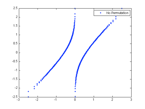
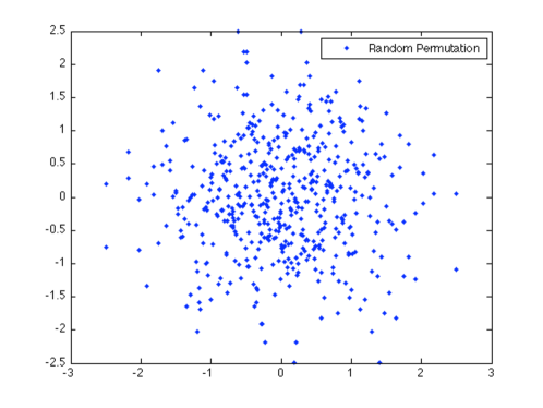
Figure 1: Scatter plots of fake Gaussian 2-dimensional density: no permutation and random permutation

Fig. 2. shows the MSE of the random permutation trellis coder for IID Gaussian at $R=1$ with various shift register length. The performance has not yet shown to hit a plateau as shift register length increases.

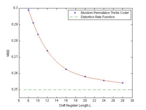
Figure 2: Performance: 1 bit Gaussian

The uniform IID source is of interest because it is simple, there is no exact formula for the rate-distortion function with respect to mean-squared error and hence it must be found by numerical means, and because one of the best compression algorithms, trellis-coded quantization (TCQ) is theoretically ideally matched to this example. So the example is an excellent one for demonstrating some of the issues raised here and for comparison with other techniques.

The Rose algorithm yielded a Shannon optimal distribution with an alphabet of size 3 for $R=1$. The points and their probabilities are shown in Table IV.

Plugging the distribution into the random permutation trellis encoder led to a mapping $g$ of (0 0.368) to 0.2, [0.368 0.632] to 0.5, and (0.632 1) to 0.8.

For the Laplacian source of variance $1$, the Rose algorithm yielded a Shannon optimal distribution with an alphabet of size 9 for the 1 bit case. The 9 reproduction points and their probabilities are listed in Table V.

$y$	$\pm$ 4.6273	$\pm$ 3.2828	$\pm$ 2.1654	$\pm$ 1.1063	0
$p_{Y}(y)$	0.0014	0.0065	0.0285	0.1266	0.6740

TABLE V: Shannon Optimal Reproduction Distribution for the Laplacian Source

For all three test sources — Gaussian, uniform, and Laplacian — the performance of the random permutation trellis source encoder is approaching the Shannon limit. Therefore, it is of interest to estimate the entropy rate of the encoder output bit sequence, which should be close to an IID equiprobable Bernoulli process since an entropy rate near 1 is a necessary condition for approximate optimality [12, 14]. A ”plug-in”(or maximum-likelihood) estimator was used for this purpose. The estimator uses the empirical probability of all words of a fixed length in the sequence to estimate the entropy rate. Bit sequences of length $10^{6}$ produced by encoding the Gaussian, uniform, and Laplacian sources with trellis encoder of shift register length $L=12$ were fed into the estimator, the resulting entropy rate estimation ranges from $0.9993$ to $0.9995$. For comparison, the estimator yielded entropy rate of 0.9998 for a randomly generated bit sequence of the same length.

Eriksson et al.’s LC results for 1 bit at 512 states (equivalent to shift register length 10) for Gaussian source is better than the random permutation results for the same shift register length. This is likely the result of their exhaustive search over all possible ways of labeling the branches within the constraint of their axioms. A similar approach to the random permutation code would be to search for the permutation that produced the best results. Our results are from randomly chosen permutations, so they reflect performance of the ensemble average (which we believe may eventually lead to a source coding theorem using random coding ideas). All permutations have the same marginals, but some permutations will have better higher order distributions. Such an optimization is feasible only for small $L$. We tested an optimization by exhaustion for $L=3$ and found that the best MSE (SNR) was 0.3262 (4.8647), while the average MSE (SNR) for all permutations was 0.3852 (4.1431). This demonstrates that the best permutation can provide notable improvement over the average, but we have no efficient search algorithm for finding optimum permutations.

Appendix A Proof of Lemma 2

The encoded and decoded processes are both stationary and ergodic since the original source is. From (7) and the source coding theorem,

$$D(f_{n},g_{n}) = E[d(X_{0},\hat{X}_{0}^{(n)})]\geq\overline{d}(\mu_{X},\mu_{\hat{X}^{(n)}})$$

$$\geq \mathop{\rm inf}_{\nu:H(\nu)\leq R}\overline{d}(\mu_{X},\nu)=D_{X}(R).$$

The second inequality follows since stationary coding reduces entropy rate, and so $R\geq{H}(U^{(n)})\geq{H}(\hat{X}^{(n)})$. Since the leftmost term converges to the rightmost, the first equality of the lemma is proved.

Standard inequalities of information theory yield

$$R\geq{H}(U^{(n)})\geq{H}(\hat{X}^{(n)})\geq{I}(X,\hat{X}^{(n)})\geq R_{X}(D(f_{n},g_{n}))$$

where the second inequality follows since mutual information rate is bounded above by entropy rate, and the third inequality follows from the process definition of the Shannon rate-distortion function [11]. Taking the limit as $n\rightarrow\infty$, the rightmost term converges to $R$ since the code sequence is asymptotically optimal (so that $D(f_{n},g_{n})\to D_{X}(R)>0$) and the Shannon rate-distortion function is a continuous function of its argument (except possibly at $D=0$). Thus $\lim_{n\rightarrow\infty}{H}(U^{(n)})=\lim_{n\rightarrow\infty}{H}(\hat{X}^{(n)})=R.$ proving the second equality of the lemma.

The final part requires Marton’s inequality [19] relating Ornstein’s $\overline{d}$ distance and relative entropy when one of the processes is IID. Suppose that $\mu_{U}$ and $\mu_{Z}$ are stationary process distributions for two processes with a common discrete alphabet and that $\mu_{U^{N}}$ and $\mu_{Z^{N}}$ denote the finite dimensional distributions. For any integer $N$ the relative entropy or informational divergence is defined by

$$H(\mu_{U^{N}}\|\mu_{Z^{N}})=\sum_{u^{N}}\mu_{U^{N}}(u^{N})\log{\mu_{U^{N}}(u^{N})\over\mu_{Z^{N}}(u^{N})}.$$

In our notation Marton’s inequality states that if $U$ is a stationary ergodic process and $Z$ is an IID process, then

$$N^{-1}\mathcal{T}_{0}(\mu_{U^{N}},\mu_{Z^{N}})\leq\left[{\ln 2\over 2N}H(\mu_{U^{N}}\|\mu_{Z^{N}}))\right]^{1/2}.$$

Since $Z$ is an IID equiprobable process with alphabet size $2^{R}$,

$$N^{-1}\mathcal{T}_{0}(\mu_{U^{N}},\mu_{Z^{N}})\leq\left[{\ln 2\over 2N}(NR-H(U^{N}))\right]^{1/2}$$

and taking the limit as $N\rightarrow\infty$ yields (in view of property (2) of the $\overline{d}$ distance)

$$\overline{d}_{0}(\mu_{U},\mu_{Z})\leq\left[{\ln 2\over 2}(R-H(U))\right]^{1/2}.$$

Applying this to $U^{(n)}$ and taking the limit using the previous part of the lemma completes the proof. $\Box$

Lemma 6

Let $\mu^{N}$ denote the $N$-fold product of a probability distribution $\mu$ on the real line such that $\int x^{2}d\mu(x)<\infty$. Assume $\{\nu_{n}\}$ is a sequence of probability distribution on $\mathbb{R}^{N}$ such that $\lim_{n\to\infty}\mathcal{T}_{2}(\mu^{N},\nu_{n})=0.$ If $Y^{(n)}_{1},Y^{(n)}_{2},\ldots,Y^{(n)}_{N}$ are random variables with joint distribution $\nu_{n}$, then for all $i\neq j$,

$$\lim_{n\to\infty}E\bigl{[}\bigl{(}Y^{(n)}_{i}-E(Y^{(n)}_{i})\bigr{)}\bigl{(}Y^{(n)}_{j}-E(Y^{(n)}_{j})\bigr{)}\bigl{]}=0.$$

Proof. The convergence of $\nu_{n}$ to $\mu^{N}$ in $\mathcal{T}_{2}$ distance implies that there exist IID random variables $Y_{1},\ldots,Y_{N}$ with common distribution $\mu$ and a sequence or $N$ random variables $Y^{(n)}_{1},Y^{(n)}_{2},\ldots,Y^{(n)}_{N}$ with joint distribution $\nu_{n}$, all defined on the same probability space, such that

$$\lim_{n\to\infty}E[(Y^{(n)}_{i}-Y_{i})^{2}]=0,\quad i=1,\ldots,N.$$ (36)

First note that this implies for all $i$

$$\lim_{n\to\infty}E[(Y^{(n)}_{i})^{2}]=E[Y_{i}^{2}].$$ (37)

Also, $\lim\limits_{n\to\infty}E|Y^{(n)}_{i}-Y_{i}|=0$ (Cauchy-Schwarz), so that for all $i$,

$$\lim_{n\to\infty}E(Y^{(n)}_{i})=E(Y_{i}).$$ (38)

Now the statement is direct convergence of the fact that in any inner product space, the inner product is jointly continuous. To be more concrete, letting $\langle X,Y\rangle=E(XY)$ and $\|X\|=[E(X^{2})]^{1/2}$ for random variables $X$ and $Y$ with finite second moment defined on this probability space, we have the bound

$$\bigl{|}\langle Y^{(n)}_{i},Y^{(n)}_{j}\rangle-\langle Y_{i},Y_{j}\rangle\bigr{|}$$

$$\leq \bigl{|}\langle Y^{(n)}_{i},Y^{(n)}_{j}-Y_{j}\rangle\bigr{|}+\bigl{|}\langle Y^{(n)}_{i}-Y_{i},Y_{j}\rangle\bigr{|}$$

$$\leq \|Y^{(n)}_{i}\|\,\|Y^{(n)}_{j}-Y_{j}\|+\|Y^{(n)}_{i}-Y_{i}\|\,\|Y_{j}\|.$$

Since $\|Y^{(n)}_{i}\|$ converges to $\|Y_{i}\|$ by (37) and $\|Y^{(n)}_{i}-Y_{i}\|$ converges to zero by (36), we obtain that $\langle Y^{(n)}_{i},Y^{(n)}_{j}\rangle$ converges to $\langle Y_{i},Y_{j}\rangle$, i.e,

$$\lim_{n\to\infty}E(Y^{(n)}_{i}Y^{(n)}_{i})=E(Y_{i}Y_{j})=E(Y_{i})E(Y_{j})$$

since $Y_{i}$ and $Y_{j}$ are independent if $i\neq j$. This and (38) imply the lemma statement. $\Box$

References

- [1] J. B. Anderson and J. B. Bodie, “Tree encoding of speech,” IEEE Trans. Inform. Thy., vol IT-21, pp. 379–387, Jul. 1975.
- [2] R. E. Blahut, “Computation of channel capacity and rate distortion functions,” IEEE Trans. Inform. Theory, vol. IT-18, pp. 460-473, Jul. 1972.
- [3] I. Csiszár, “On an extremum problem in information theory,” Studia Scientiarum Mathematicarum Hungarica, vol. 9, no. 1–2, pp. 57–71, 1974.
- [4] T. Eriksson, J.B. Anderson, and N. Goertz, “ Linear congruential trellis source codes: design and analysis,” IEEE Transactions on Communications, vol. 55, no. 9, pp. 1693–1701, Sept. 2007.
- [5] W. A. Finamore and W. A. Pearlman. “Optimal encoding of discrete-time, continuous-amplitude, memoryless sources with finite output alphabets,” IEEE Trans. Inform. Theory, vol. IT-26, pp. 144–155, Mar. 1980.
- [6] S. L. Fix, “Rate distortion functions for squared error distortion measures,” in Proc. 16th Annu. Allerton Conf. Commun., Contr., Comput., Oct. 1978.
- [7] R. G. Gallager, Information Theory and Reliable Communication, John Wiley and Sons, New York, 1968.
- [8] A. Gersho and R. M. Gray, Vector Quantization and Signal Compression, Kluwer Academic Press, 1992.
- [9] R. M. Gray, “Sliding–block source coding,” IEEE Trans. Inform. Theory, vol. IT–21, no. 4, pp. 357–368, Jul. 1975.
- [10] R. M. Gray, “Time–invariant trellis encoding of ergodic discrete–time sources with a fidelity criterion,” IEEE Trans. Inform. Theory, vol. IT–23, pp. 71–83, Jan. 1977.
- [11] R. M. Gray, Entropy and Information Theory, Springer–Verlag, New York, 1990. Second Edition, Springer, 2011.
- [12] R. M. Gray, “Source coding and simulation,” IEEE Information Theory Society Newsletter, vol. 58, no. 4, Dec. 2008.
- [13] R. M. Gray, Probability, Random Processes, and Ergodic Properties: Second Edition, Springer, New York, 2009.
- [14] R. M. Gray and T. Linder, “Bits in asymptotically optimal lossy source codes are asymptotically Bernoulli,” Proc. 2009 Data Compression Conference (DCC), pp. 53–62, Mar. 2008.
- [15] R. M. Gray, D. L. Neuhoff and P. C. Shields, “A generalization of Ornstein’s d–bar distance with applications to information theory,” Annals of Probability, vol. 3, no. 2, pp. 315–328, Apr. 1975.
- [16] R. M. Gray, D. L. Neuhoff and D. S. Ornstein, “Nonblock source coding with a fidelity criterion,” Annals of Probability, vol. 3, no. 3, pp. 478–491, Jun. 1975.
- [17] Y. Linde and R. M. Gray, “A fake process approach to data compression,” IEEE Trans. Commun., vol. COM–26, pp. 840–847, Jun. 1978.
- [18] M. Marcellin and T. Fischer, “Trellis coded quantization of memoryless and Gauss-Markov sources,” IEEE Trans. Commun., vol. 38, no. 1, pp. 92–93, Jan. 1990.
- [19] K. Marton, “Bounding distance by informational divergence: a method to prove measure concentration,” Annals of Probability, vol. 24, pp. 857–866, 1997.
- [20] P. Noll and R. Zelinski, “Bounds on quantizer performance in the low bit-rate region,” IEEE Trans. Commun., vol. COM-26, no. 2, pp. 300-304, Feb. 1978.
- [21] D. Ornstein, “An application of ergodic theory to probability theory,” Annals of Probability, vol. 1, no. 1, pp. 43–58, 1973.
- [22] D. Ornstein, Ergodic Theory, Randomness, and Dynamical Systems, Yale University Press, New Haven, 1975.
- [23] W. A. Pearlman, “Sliding-block and random source coding with constrained size reproduction alphabets,” IEEE Trans. Commun., vol. COM-30, no. 8, pp. 1859-1867, Aug. 1982.
- [24] M. S. Pinsker, “Information and information stability of random variables and processes,” Holden Day, San Francisco, 1964.
- [25] S. T. Rachev and L. Rüschendorf, Mass Transportation Problems Vol. I: Theory, Vol. II: Applications. Probability and its applications. Springer-Verlag, New York, 1998.
- [26] K. Rose, “A mapping approach to rate-distortion computation and analysis,” IEEE Trans. Inform. Theory, vol. 40, no. 6, pp. 1939–1952, Nov. 1994.
- [27] C. E. Shannon, “Coding theorems for a discrete source with a fidelity criterion,” IRE National Convention Record, Part 4, pp. 142–163, 1959.
- [28] P. C. Shields, “Stationary coding of processes,” IEEE Trans. Inform. Theory, vol. 25, no. 3, pp. 283–291, May 1979.
- [29] L. Stewart, Trellis data compression, Ph.D. dissertation, Dep. Elec. Eng., Stanford Univ., Stanford, CA 94305, June 1981.
- [30] L. Stewart, R. M. Gray, and Y. Linde, “The design of trellis waveform coders,” IEEE Trans. Commun., vol. COM-30, no. 4, pp. 702-710, Apr. 1982.
- [31] Y. Steinberg and S. Verdú, “Simulation of random processes and rate-distortion theory,” IEEE Trans. Inform. Theory, vol. 42, no. 1, pp. 63–86. Jan. 1996.
- [32] R. J. van der Vleuten and J. H. Weber, “Construction and evaluation of trellis-coded quantizers for memoryless sources,” IEEE Trans. Inform. Theory, vol. 41, no. 3, pp. 853–87 , May 1995.
- [33] C. Villani, Optimal Transport, Old and New, Grundlehren der mathematischen Wissenschaften, vol. 338, Springer 2009.
- [34] A. J. Viterbi and J. K. Omura, “Trellis Encoding of Memoryless Discrete-Time Sources with a Fidelity Criterion,” IEEE Trans. Inform. Theory, vol. IT-20, no. 3, May 1974.
- [35] S. G. Wilson and D. W. Lytle, “Trellis coding of continuous-amplitude memoryless sources,” IEEE Trans. Inform. Theory, vol. IT-23, pp. 404–409, May 1977.
- [36] E-h. Yang and Z. Zhang, “Variable-Rate Trellis Source Encoding,” IEEE Trans. Inform. Theory, vol. IT-45, No. 2, pp.586–608, March 1999.