Heavy pseudoscalar mesons in a Schwinger-Dyson–Bethe-Salpeter approach

Abstract

The mass spectrum of heavy pseudoscalar mesons, described as quark-antiquark bound systems, is considered within the Bethe-Salpeter formalism with momentum-dependent masses of the constituents. This dependence is found by solving the Schwinger-Dyson equation for quark propagators in rainbow-ladder approximation. Such an approximation is known to provide both a fast convergence of numerical methods and accurate results for lightest mesons. However, as the meson mass increases, the method becomes less stable and special attention must be devoted to details of numerical means of solving the corresponding equations. We focus on the pseudoscalar sector and show that our numerical scheme describes fairly accurately the $\pi$, $K$, $D$, $D_{s}$ and $\eta_{c}$ ground states. Excited states are considered as well. Our calculations are directly related to the future physics programme at FAIR.

1 Introduction

The description of mesons as quark-antiquark bound states within the framework of the Bethe-Salpeter equation with momentum dependent quark masses, determined by the Schwinger-Dyson equation, is able to explain successfully many spectroscopic data [1, 2, 3, 4, 5, 6, 7, 8, 9]. Contrarily to traditional phenomenological models, like quark bag models, the presented formalism maintains important features of QCD, such as dynamical chiral symmetry breaking, dynamical quark dressing, requirements of the renormalization group theory etc. The main ingredients here are the full quark-gluon vertex function and the dressed gluon propagator, the calculation of which is entirely determined by the running coupling and the bare quark masses. In principle, if one were able to solve the Schwinger-Dyson equation within all pQCD orders, the approach would not depend on any free parameters. However,due to known technical problems, one restricts oneself to calculations of the few first terms of the perturbative series, usually up to the one-loop approximation. The obtained results, which formally obey all the fundamental requirements of the theory, are then considered as exact ones with, however, effective parameters. This is known as the rainbow-ladder approximation for the Schwinger-Dyson equation. The merit of the approach is that, once the effective parameters are fixed, the whole spectrum of known mesons is supposed to be described on the same footing: including also excited states.

It should be noted that there exists other approaches based on the same physical ideas but not so sophisticated, e.g. employing simpler interactions, such as a separable interaction for the effective coupling [6]. Such approaches describe fairly well the properties of light mesons, nevertheless, investigation of heavier mesons and excited states, consisting even of light (u,d,s) quarks, requires implementations of more accurate numerical methods to solve the corresponding equations. Among other successful efforts in this realm the Refs. [10, 11] must be also mentioned.

In the present note we are going to apply the combined Schwinger-Dyson and Bethe-Salpeter (BS) formalisms to describe the meson mass spectrum including heavy mesons and excited states as well. Particular attention is paid to the charm sector which, together with the baryon spectroscopy, is a major topic in the FAIR research programme. Two large collaborations at FAIR [12, 13] plan precision measurements. Note, that it becomes now possible to experimentally investigate not only the mass spectrum of the mentioned mesons, but also different processes of their decay, which are directly connected with fundamental QCD problems (e.g., $U(1)$ axial anomaly, transition form factors etc.) and with the known problem of changing the meson characteristics at finite temperatures. The latter is crucial in understanding the di-lepton yields in nucleus-nucleus collisions at, e.g. HADES. All these circumstances require an adequate theoretical foundation to describe the meson spectrum and the meson covariant wave functions (i.e. the BS partial amplitudes) needed in calculations of the relevant Feynman diagrams and observables.

Our paper is organized as follows. In section 2, the parametrization of the gluon propagator is presented and the Schwinger-Dyson equation for the quark propagator is discussed. Section 3 deals with the Bethe-Salpeter equation. Numerical results are discussed in Section 4. Conclusions are drawn in section 5.

2 Propagators and Schwinger-Dyson equation

The Bethe-Salpeter and Schwinger-Dyson equations in Minkowski space contain poles and branch-point singularities which strongly hinder the procedure of finding numerical solutions. Usually, to avoid these difficulties, one performs the Wick rotation and formulates the corresponding equations in Euclidean space, where all singularities in amplitudes and propagators are removed, so that the equations can be solved numerically. The known Mandelstam technique allows then to calculate matrix elements of observables which, being analytical functions of the relative energy, are the same in both Minkowski and Euclidean spaces.

In our case we consider the Schwinger-Dyson equation for the quark propagator within pQCD with summing all diagrams up to one-loop. In calculations of diagrams the chiral symmetry breaking is implemented from the very beginning [9]. The exact results, even only up to one-loop diagrams, after proper regularization and renormalization procedures are rather cumbersome for further numerical calculations. Nevertheless, in practical calculations one can employ reasonable parametrizations for the corresponding vertices and propagators to find solutions numerically. So, a phenomenological expression, inspired by calculations of the mentioned diagrams and preserving the requirements of the theory, for the combined running coupling and gluon propagator has been suggested in Ref. [9]

$$g^{2}(k^{2})D_{\mu\nu}(k^{2})=\left(\frac{4\pi^{2}Dk^{2}}{\omega^{2}}e^{-k^{2}/\omega^{2}}+\frac{8\pi^{2}\gamma_{m}F(k^{2})}{ln[\tau+(1+\frac{k^{2}}{\Lambda_{QCD}^{2}})]}\right)\left(\delta_{\mu\nu}-\frac{k_{\mu}k_{\nu}}{k^{2}}\right)\>,$$ (1)

where the first term originates from the infrared (IR) part of the interaction determined by non-pertubative effects, while the second one ensures the correct ultraviolet asymptotics. Accordingly to the known fact that the contribution of the IR part is predominant for formation of bound states, in what follows we neglect the second term and restrict ourselves to the IR one. Then, as seen from Eq. (1), we are left with only two effective parameters, $D$ and $\omega$.

The calculation of the renormalized Feynman diagrams leads to a fermion propagator depending on two additional parameters. In canonical calculations these are the renormalization constant $Z_{2}$ and the self-energy corrections $\Sigma(p)$. Usually, for further simplifications of calculations, instead of $Z_{2}$ and $\Sigma(p)$ one introduces other two quantities $A(p)$ and $B(p)$ in terms of which the quark propagator $S_{q}(p)$ reads as

$$S_{q}^{-1}(p)=i\gamma\cdot pA(p)+B(p);\quad\quad S_{q}(p)=\frac{-i\gamma\cdot pA(p)+B(p)}{p^{2}A^{2}(p)+B^{2}(p)}\>.$$ (2)

Then with such a representation of the quark propagator the Schwinger-Dyson equation in Euclidean space has the form (cf. Refs. [7, 9])

$$S_{q}^{-1}(p)=i\gamma\cdot p+\tilde{m}+\frac{4}{3}\int\frac{d^{4}l}{(2\pi)^{4}}\left[g^{2}D(p-l)\right]_{\mu\nu}\gamma_{\mu}S_{q}(l)\gamma_{\nu}\>,$$ (3)

where $\tilde{m}$ is the bare quark mass and the effective kernel $D(p-l)$ is

$$D(k^{2})_{\mu\nu}=\frac{4\pi^{2}Dk^{2}}{\omega^{2}}e^{-k^{2}/\omega^{2}}\left(\delta_{\mu\nu}-\frac{k_{\mu}k_{\nu}}{k^{2}}\right).$$ (4)

Note that (3) is a four dimensional integral equation. To solve it one usually decomposes the kernel over a complete set of basis functions, performs analyticaly some angular integrations and considers a new system of equations relative to such a partial decomposition. In our calculations we expand the interaction kernel into hyperspherical harmonics

$$D((p-l)^{2})=D(p^{2},l^{2},|p||l|\cos\gamma)=\sum\limits_{n}D_{n}(p,l)C^{1}_{n}(\cos\gamma)\>,$$

$$D_{n}(p,l)=\frac{2}{\pi}\int\limits_{-1}^{1}D(p^{2},l^{2},p\cdot l\cdot t)C^{1}_{n}(t)\sqrt{1-t^{2}}dt\>,$$ (5)

where $C_{n}^{1}(t)$ are the Chebyshev polynomials. For the employed ansatz of the gluon propagator the angular integration can be performed analytically leading to

$$D_{n}(p,l) =(n+1)8\pi^{2}De^{-x}\left[\frac{x-n}{z}I_{n+1}(z)-I_{n+2}(z)\right]\>,$$ (6)

$$D^{\prime}_{n}(p,l) =(n+1)4\pi^{2}\frac{D}{\omega^{2}}e^{-x}\frac{I_{n+1}(z)}{z}$$ (7)

with $x=(p^{2}+l^{2})/\omega^{2}$, $z=2pl/\omega^{2}$ and $I_{n}(z)$ being the modified Bessel functions of the first kind. In Eq. (7) $D^{\prime}_{n}(p,l)$ denotes the corresponding part of the kernel $D(k^{2})/k^{2}$. Eventually, the system of equations to be solved reads as

$$A(p) = 1+\frac{4}{3p}\int\frac{dll^{4}}{16\pi^{2}}\frac{A(l)}{l^{2}A^{2}(l)+B^{2}(l)}D_{1}(p,l)+$$

$$\int\frac{dll^{4}}{16\pi^{2}}\frac{A(l)}{l^{2}A^{2}+B^{2}}[\frac{8}{3}(p+\frac{l^{2}}{p})D^{{}^{\prime}}_{1}(p,l)-\frac{4}{3}l(D_{2}^{{}^{\prime}}(p,l)+5D_{0}^{{}^{\prime}}(p,l))]\>,$$

$$B(p) = \tilde{m}+4\int\frac{dll^{3}}{8\pi^{2}}\frac{B(l)}{l^{2}A^{2}(l)+B^{2}(l)}D_{0}(p,l)\>.$$ (8)

The resulting system of equations on (8) is a system of one-dimensional integrals and can be solved numerically, e.g. by an iteration method. We found that iteration procedure for (8) converges rather fast and practically does not depend up on the choice of the trial functions for $A(p)$ and $B(p)$. The numerical solution of (8) with the effective parameters from Ref. [7, 9] is shown in Fig. 1 as the momentum dependence of the mass $m(p)=B(p)/A(p)$ of the dressed quark for different quark flavors, i.e. for different bare masses: $\tilde{m}=0.005$ GeV for $u(d)$, $\tilde{m}=0.115$ GeV for $s$ and $\tilde{m}=1$ GeV for $c$ quarks [7]. In principle, the asymptotic behavior of $A(p)$ and $B(p)$ for large momenta can be obtained directly from (8) and, as an additional check of the method, compared with the corresponding numerical results.

Figure 1: The solution of the Schwinger-Dyson equation for the quark mass $m(p)=B(p)/A(p)$ as a function of momentum for different flavors, i.e. for the input bare quark masses $\tilde{m}$. At asymptotically large values of $p$ the mass of the dressed quark tends to its bare value.

3 Bethe-Salpeter vertex function

To determine the bound state mass of a quark-antiquark pair one needs to solve the Bethe-Salpeter equation. In rainbow-ladder approximation and in Euclidean space it reads [7, 9]

$$\Gamma(P,p)=(-\frac{4}{3})\int\frac{d^{4}k}{(2\pi)^{4}}\gamma_{\mu}S(k_{+})\Gamma(P,k)S(k_{-})\gamma_{\nu}(g^{2}D(p-k))_{\mu\nu}\>,$$ (9)

with $\Gamma$ being the Bethe-Salpeter vertex function. The color structure has been factorized explicitly. $P$ means the total momentum of the bound state, $p(k)$ is the relative momentum within the quark pair and $k_{+}=k+\xi P$, $k_{-}=k+(\xi-1)P$. The result does not depend on $\xi$ due to the covariance of the Bethe-Salpeter equation. We choose $\xi=0.5$. However, approximations might destroy covariance and one has to check a posteriori the stability of the results.

Equation (9) is written in matrix form, i.e. the vertex function $\Gamma(P,k)$ is a 4x4 matrix and, therefore, may contain 16 different functions. The general structure of the vertex functions describing bound states of spinor particles has been investigated in detail, for example, in [14]. $\Gamma$ can be expanded into functions which in turn are determined by angular momentum and parity of the corresponding meson:

$$\Gamma(p_{4},{\mbox{\boldmath$p$}}) = \sum\limits_{\alpha}g_{\alpha}(p_{4},|{\mbox{\boldmath$p$}}|)\,{\cal T}_{\alpha}({\mbox{\boldmath$p$}})\>.$$ (10)

For pseudoscalar mesons there are 4 independent angular momentum functions ${\cal T}_{\alpha}(p)$ given by

$${\cal T}_{1}({\mbox{\boldmath$p$}})=\frac{\gamma_{5}}{\sqrt{16\pi}},\quad{\cal T}_{2}({\mbox{\boldmath$p$}})=\frac{\gamma_{0}\gamma_{5}}{\sqrt{16\pi}},\quad{\cal T}_{3}({\mbox{\boldmath$p$}})=\frac{1}{\sqrt{16\pi}}\frac{({\mbox{\boldmath$p$}}{\mbox{\boldmath$\gamma$}})}{|{\mbox{\boldmath$p$}}|}\gamma_{0}\gamma_{5},\quad{\cal T}_{4}({\mbox{\boldmath$p$}})=\frac{1}{\sqrt{16\pi}}\frac{({\mbox{\boldmath$p$}}{\mbox{\boldmath$\gamma$}})}{|{\mbox{\boldmath$p$}}|}\gamma_{5}\>.$$ (11)

Our choice differs from the standard expansion [9]. The main advantage of (11) is orthogonality $\int d\Omega_{p}Tr[{\cal T}_{m}({\mbox{\boldmath$p$}}){\cal T}_{n}^{+}({\mbox{\boldmath$p$}})]=\delta_{mn}$.

This property immediately allows to get a system of linear integral equations for the functions $g_{\alpha}(p_{4},{\mbox{\boldmath$p$}})$. As in the case of the Schwinger-Dyson equation, for these functions we employ also the hyperspherical harmonics

$$X_{kl}(\chi)=2^{l}l!\sqrt{\frac{2}{\pi}}\sqrt{\frac{(k+1)(k-l)!}{(k+l+1)!}}\sin^{l}\chi C_{k-l}^{l+1}(\cos\chi)$$ (12)

which separates the angular dependence

$$g_{i}(p4,|{\mbox{\boldmath$p$}}|)=\sum_{j}g^{j}_{i}(p)X_{j,0(1)}(\chi_{p})$$ (13)

and, hence, allows to perform the angular integration leaving us with a set of coupled one-dimensional linear integral equations for the functions $g^{k}_{i}(p)$

$$g_{i}^{k}(p)=\int_{0}^{\infty}\frac{dkk^{3}}{4\pi^{2}}\sum A_{ij}^{km}(p,k)g_{j}^{m}(k)$$ (14)

where $p$($k$) is the length of the Euclidean 4-momentum, $p=\sqrt{p_{4}^{2}+{\mbox{\boldmath$p$}}^{2}}$. The matrices $A_{ij}^{km}(p,k)$ can be calculated analytically.

The series (13) converges rather fast and in practice only few terms need to be taken into account. Then by choosing a suitable method of integration, e.g. Gaussian quadrature, the system of equations (14) can be written as a system of homogeneous linear equations. Schematically, it can be written in the form

$$g=Kg\>.$$ (15)

The condition ${\rm det}(K-1)=0$ is sufficient for the existence of a bound state. Hence, formally the zeros of the determinant ${\rm det}(K-1)$ determine the solution of the BS equation, including also excited states. In our case, for the sake of increasing the accuracy, for the standard Gaussian quadrature we use a mapping

$$k=k_{0}\frac{1+x}{1-x}\>,$$ (16)

where $k_{0}$ weights the integrand and $x\in[-1,1]$ is the integration variable (cf. Ref. [15]).

Here an important moment is worth to be emphasized. Usually, when solving the BS equation for constituent particles, i.e. for particles with constant masses, the resulting system of partial equations is real. In case of momentum dependent masses the Bethe-Salpeter equation becomes complex and requires the knowledge of the quark propagator for complex momenta $k_{\pm}$ (where $k_{\pm}=\frac{1}{2}P\pm k$ are the momenta of quarks) and, hence, requires to solve the Schwinger-Dyson equation also for complex momenta. For small meson masses (e.g. $M\approx 500$ MeV) only a small energy region contributes to the integral in Eq. (14), $k<1$ GeV. In this case the propagator functions can be obtained by using the solution for real momenta, and afterwards $A(p)$ and $B(p)$ are calculated at complex momenta from (8) [3, 7]. For heavier states, $M>1$ GeV, the imaginary part of the quark momenta, Im $k_{\pm}$, becomes rather large and the integrand in (8) rapidly oscillates as a function of $k$, hindering an accurate computation of the integral.

To avoid this problem a witty trick has been suggested in Ref. [8]. It is based on the observation that, as seen from the Schwinger-Dyson equation, all the values of the momenta $k_{\pm}^{2}$ are located within a domain limited by a parabola, as shown in Fig. 2.

Figure 2: Integration contour of (17). Branches of parabola are determined by ${\rm Re}k_{\pm}^{2}=-M^{2}/4-k^{2}$ and ${\rm Im}k_{\pm}=\pm Mk$. Since the integration domain is infinite, in concrete calculations one shall restrict to some large, but finite values of $k^{2}$; the vertical line illustrates such a cut of the infinite domain in practical calculations.

Then, due to the Cauchy’s theorem, it suffices to know the solution along this parabola to be able to compute it everywhere inside the corresponding domain:

$$2\pi iA(z_{1})=\oint dz\frac{A(z)}{z-z_{1}}\>.$$ (17)

Shifting the integration variable $l\rightarrow p-l$, (8) can be solved directly along this contour. For large real part of the momentum the asymptotic form of $A$ and $B$ can be also used. It should be noted that the described procedure of solving numerically the equations works quite well if the integration domain is chosen in a reasonable way, i.e. large enough to assure good asymptotics, but not too large, as the accuracy of the solution decreases with increasing integration domain (certainly, at a given Gaussian mesh). Note also, that asymptotic behaviors of the functions $A$ and $B$ is essential for heavier quarks, see Fig. 1.

4 Numerical results

As an example of our numerical study we exhibit in Fig. 3 the energy of the lowest bound states of a hypothetical meson $qq_{x}$ consisting of one given quark $q$ with the mass known from the Schwinger-Dyson equation, bound with a second quark $q_{x}$ for which the input bare mass $\tilde{m}_{x}$ is let to vary arbitrarily. The corresponding effective parameters have been chosen as $\omega=0.5$ GeV and $D=16$ GeV^-2 [7, 9] and the bare masses for $q$ correspond to $(u,d,s)$ quarks, q=u (with $\tilde{m}_{u}=0.005$ GeV), q=s (with $\tilde{m}_{s}=0.115$ GeV) and q=c (with $\tilde{m}_{c}=1.0$ GeV). This figure illustrates the whole mass spectrum of pseudoscalar mesons with masses up to $3\,\,GeV/c^{2}$. So, if the $q_{x}$ quark corresponds to a $c$ quark, then at the intersection of the vertical line $\tilde{m}_{x}=m_{c}$ ($\approx 1\,\,GeV/c^{2}$) with ”$ux$” curve one obtains the $D$ -meson (with the quark contents a$uc$), with the ”$sx$” curve the $D_{s}$ meson and with the ”$cx$” curve - the $\eta_{c}$ meson, respectively. It is worth noting that the ”$ux$” curve crosses the $\tilde{m}_{u}=0.115$ GeV line roughly at the same value of $M_{qq_{x}}$ as the ”$sx$” curve crosses the $\tilde{m}_{u}=0.005$ GeV line, thus proving a check of consistency of the approach and, at the same time, describing correctly the lowest pseudoscalar $us$ state corresponding to the K meson. It can be seen that even without a fine tuning of $\tilde{m}_{s,c}$ the meson mass spectrum is reproduced fairly well: 135 MeV ($\pi^{0}$ meson), 497 MeV ($K$ meson), 1870 MeV ($D^{\pm}$ meson), 1970 MeV ($D_{s}^{\pm}$ meson) and 2980 MeV ($\eta_{c}$ meson).

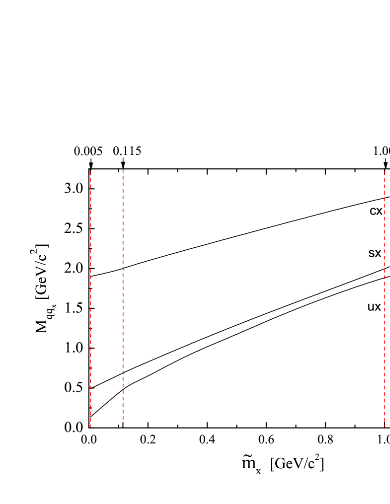
Figure 3: The bound state masses of a system $qq_{x}$ as a function of the bare mass $\tilde{m}_{x}$, the other quark being either a $u$ quark with $\tilde{m}_{u}=0.005$ GeV (the curve labeled as ”$ux$”) or a strange quark with $\tilde{m}_{s}=0.115$ GeV (the curve labeled as ”$sx$”) or a charm quark with $\tilde{m}_{c}=1.0$ GeV (the curve labeled as ”$cx$”). The effective parameters are $\omega=0.5$ GeV and $D=16$ GeV^-2. The masses of pseudoscalar $\pi$ $K$, $D$, $D_{s}$ and $\eta_{c}$ mesons according to [17] are indicated at the right side. The vertical dashed lines mark the selected bare quark masses for $u$, $s$, and $c$.

In nature, a pseudoscalar $s\bar{s}$ meson with simple quark structure does not exist. However, our ”$sx$” curve intersects with the bare mass of the $s$-quark, i.e. the approach predicts an existence of $s\bar{s}$ meson around 600 MeV. This can be considered as a ”ghost” state, or as check of consistency of the approach. Apart from this circumstance, it is amazing that the simple two-parameter ansatz of the gluon propagator in the IR region together with the Schwinger-Dyson equation in rainbow approximation delivers such a quark propagator which, via the Bethe-Salpeter equation in rainbow-ladder approximation, results in such a nice description of pseudoscalar $\pi$, $K$, $D$, $D_{s}$ and $\eta_{c}$ states.

Clearly, a special parameterization of the gluon propagators with two adjusted quantities and the self consistent determination of three bare quark masses serve as input for obtaining finally five pseudoscalar meson masses. The straight forward extension to the scalar, vector and axialvector mesons without further adjustments will provide the ultimate test for the subtleties of the numerical implementation of the employed theoretical scheme and the inherent approximations. Work along this line is in progress.

Masses of excited states, which correspond to radial excitations of the considered mesons, can be evaluated in a similar way, i.e. by finding of the next zeros of the determinant (15). As our analysis shows, the determinant changes monotonously with increasing mass. So that, naively, one would not expect a bound state of a $u\bar{u}$ system with mass larger than 800 MeV, since even at zero momenta, the maximum constituent quark mass is around 400 MeV, cf. Fig. 1. However, in the deeply non-Euclidean domain, which corresponds to $k_{+}^{2}\simeq-M^{2}/4$ (Fig. 2), the dynamical quark masses, contrubiting to the BS equation, increase till 600-700 MeV depending on $M$. Hence, the Schwinger-Dyson equation allows to understand the formation mechanism of such bound states which, from the constituent quark model point of view, can not be even predicted a priori. The mass of the first excited $u\bar{u}$ state is found to be 1080 MeV, i.e. significantly above the maximum mass from the Schwinger-Dyson equation alone. Analogously, for the $c\bar{u}$ system, the first excited state is found to be around 2530 MeV, which is in a good agreement with data. Similar results have been obtained in other groups, see Ref. [10].

Note that in solving the BS equation for the mass spectrum of mesons we obtain also the partial BS amplitudes which can be used in calculations of various dynamical observables, such as the meson life-time, transition form factors, the dependence of the meson widths up on temperature of an ambient medium etc. Such investigations are in progress and results will be reported elsewhere.

5 Conclusion

The method of solving the Schwinger-Dyson equation in rainbow-ladder approximation in Euclidean space by using the hyperspherical harmonics basis is proposed. The obtained numerical solutions are then used to solve the Bethe-Salpeter equation for the meson mass spectrum in a large interval of meson masses. In solving the Bethe-Salpeter equation a new set of basis functions has been used which allows a further easy decomposition of the Bethe-Salpeter vertex functions into hyperspherical harmonics basis

The obtained mass spectrum for pseudoscalar mesons in a wide range, ranging from pions to $\eta_{c}$ mesons, is in a good agreement with experimental data. Excited states were considered as well and found to be also in a good agreement with experimental data and with calculations by other groups. By solving the Bethe-Salpeter equation, the corresponding partial wave functions are also obtained which will allow, in future, to calculate a variety of observables related to physical programmes at, e.g. FAIR.

References

- [1] Jain P., Munczek H.J.: Phys. Rev. D 44, p. 1873, 1991
- [2] Munczek H.J., Jain P.: Phys. Rev D 46, p. 438, 1992
- [3] Maris P., Roberts C.D.: Phys. Rev. C 56, p. 3369, 1997
- [4] Frank M.R., Roberts C.D.: Phys. Rev. C 53, p. 390-398, 1996
- [5] Tandy P.: Prog. Part. Nucl. Phys. 39, p. 117, 1997
- [6] Horvatic D., Blaschke D., Klabucar D., Radzabov A.E.: Phys. Part. Nucl. 39, p. 1033-1039, 2008
- [7] Alkofer R., Watson P., Wiegel H.: Phys. Rev. D 65, 094026, 2002
- [8] Fisher C.S., Watson P., Cassing W.: Phys. Rev. D 72, p. 094025, 2005
- [9] Roberts C.D., Bhagwat V.S., Wright S.V., Holl A.: Eur. Phys. J. ST 140, p. 53-116, 2007
- [10] Krassnigg A.: Phys. Rev. D 80, 114010, 2009
- [11] Souchlas N.: arXiv:1006.0942v1 [nucl-th]
- [12] CBM Collaboration, http://www.gsi.de/fair/experiments/CBM/index_e.html.
- [13] PANDA Collaboration, http://www-panda.gsi.de/auto/phy/_home.htm.
- [14] Kubis J.J.: Phys. Rev D 6, p. 547, 1972
- [15] Dorkin S.M., Beyer M., Semikh S.S., Kaptari L.P.: Few Body Syst. 42, p. 1-32, 2008
- [16] Ioakimidis N.I., Papadakis K.E., Perdios E.A.: BIT 31, p. 276, 1991
- [17] Nakamura K. et al., J. Phys. G 37, 075021, 2010