ANALYSIS OF A STATE CHANGING SUPERSOFT X-RAY SOURCE IN M31

Abstract

We report on observations of a luminous supersoft X-ray source (SSS) in M31, r1-25, that has exhibited spectral changes to harder X-ray states. We document these spectral changes. In addition, we show that they have important implications for modeling the source. Quasisoft states in a source that has been observed as an SSS represent a newly-discovered phenomenon. We show how such state changers could prove to be examples of unusual black hole or neutron star accretors. Future observations of this and other state changers can provide the information needed to determine the nature(s) of these intriguing new sources.

1 INTRODUCTION

Luminous supersoft X-ray sources (SSSs) were established as a class by ROSAT observations of roughly 30 sources in the Magellanic Clouds, Milky Way, and M31 (Greiner, 2000). Chandra and XMM-Newton observations of external galaxies have now discovered hundreds of soft X-ray sources with properties that both exemplify and extend the class of SSSs (e.g., Di Stefano et al., 2003; Kong & Di Stefano, 2003; Di Stefano et al., 2003; Di Stefano & Kong, 2004; Greiner et al., 2004; Di Stefano et al., 2006, 2010; Orio et al., 2010; Liu, 2011). Even though they are bright, with luminosities higher than $10^{36}$ erg s^-1, we know of only a handful in the Galaxy, because the radiation they emit is readily absorbed by the interstellar medium. In fact, the SSSs used to define the class display little or no emission above $1$ keV. Roughly a dozen SSSs are known in the Magellanic Clouds (Greiner, 2000). Some of these are associated with novae, and are clearly hot white dwarfs (see Greiner, 2000). In M31, some SSSs have been shown to be associated with supernova remnants and novae (Orio et al., 2010; Pietsch et al., 2005, 2007; Stiele et al., 2010).

The most mysterious component of the class is comprised of X-ray binaries, most with orbital periods of a day or less. A promising model for these sources is one in which their prodigious luminosities are produced by the nuclear burning of matter accreted by a white dwarf (van den Heuvel et al., 1992; Rappaport et al., 1994). Nuclear burning should allow the white dwarf to retain accreted matter and increase in mass. Binary SSSs have therefore been suggested as progenitors of accretion-induced collapse (van den Heuvel et al., 1992) and of Type Ia supernovae (Rappaport et al., 1994). Nuclear-burning white dwarfs in wider orbits are also expected (Hachisu et al., 1996; Di Stefano & Nelson, 1996). Indeed, symbiotic binaries have been observed as SSSs (e.g., Greiner, 2000; Orio et al., 2007).

Because it is difficult to detect SSSs in the Milky Way, and the Magellanic Clouds are too small to host a large population, it is important to search for SSSs in external galaxies. The advent of Chandra and XMM-Newton has made such searches possible. Hundreds of SSSs have now been discovered, some in galaxies as far from us as the Virgo cluster (Liu, 2011). As the numbers of SSSs has increased, we have begun to find evidence of sources that have properties different from those of the SSSs that established the class. Some SSSs are hundreds of times more luminous than the Eddington limit for a Chandrasekhar-mass white dwarf. Several of these ultraluminous supersoft sources are candidates for accreting black holes (Di Stefano et al., 2004; Kong et al., 2004; Kong & Di Stefano, 2005; Mukai et al., 2005; Liu & Di Stefano, 2008). In addition, the search for the softest sources has identified a class of sources that are significantly harder than SSSs, yet also significantly softer than canonical X-ray sources: quasisoft X-ray sources (QSS; Di Stefano et al., 2004; Di Stefano & Kong, 2003; Di Stefano et al., 2004). QSSs have luminosities above $10^{36}$ ergs s${}^{-1},$ but emit few or no photons with energy above $2$ keV. Some could be hot white dwarfs in which there is an additional hard component and/or which are highly absorbed. Those fitting this model are good candidates for progenitors of Type Ia supernovae, because they would likely correspond to the most massive nuclear-burning white dwarfs (e.g., Rappaport et al., 1994; Di Stefano, 2010, references). Others are too hot to be white dwarfs and may correspond to either black holes or neutron stars.

In this paper we report on a source (r1-25) that has been observed to switch between SSS and QSS states (Stiele et al., 2008, 2010; Di Stefano et al., 2010; Orio et al., 2010). Unlike M101-ULX-1 (e.g., Kong et al., 2004; Kong & Di Stefano, 2005; Mukai et al., 2005), a well known state changing source, r1-25 is not ultraluminous. r1-25 is unique in that no such sources are known in the Galaxy or Magellanic Clouds. We examined all available Chandra, Swift, and optical data from Hubble Space Telescope (HST) and the Local Group Survey (LGS) for this source. We also checked the literature for XMM-Newton observations and analysis of the source. The question we want to answer is: what is the physical nature of this unique source?

We analyze the X-ray data for the source in $\S$2. In $\S$3, we present evidence that the source changes state. In $\S$4, we analyze the optical data. We discuss the possible models that fit this source in $\S$5.

2 X-ray Observations and Analysis

The source r1-25 has been discussed in the literature (Kong et al., 2002; Williams et al., 2004; Di Stefano et al., 2004; Kaaret, 2002; Voss & Gilfanov, 2007; Stiele et al., 2010; Di Stefano et al., 2010; Orio et al., 2010). It is located in the central region of M31 approximately $0.4\arcmin$ (about 91 parsecs) from the nucleus. The coordinates of the source are (J2000.0) RA = 00:42:47.90, DEC = +41:15:49.99. This region of M31 has been well sampled over the past 13 years. For this paper, we searched the Chandra archive for all public observations of r1-25 through June 2, 2009. There were 86 observations that covered the source. r1-25 was detected in 45 observations (28 ACIS-I, 2 ACIS-S, and 15 HRC-I observations) from August 8, 2000 to March 11, 2009. We note that the source position was the same in all detections, and we are confident that r1-25 is one source. We supplemented the Chandra data with Swift observations of the region in 2009. However, the source was off during the Swift observations, which are not included in this paper.

Liu (2011) presented the photometry for the ACIS observations of r1-25 taken between 2000 and 2004. We analyzed the ACIS data taken between 2004 and 2009 using the method presented in that paper. We used CIAO version 4.1.2 (Fruscione et al., 2006) to analyze the recent data. For source detection, we used CIAO tool wavdetect (Freeman et al., 2002; Fruscione et al., 2006). Only photons between 0.3-7 keV were considered and the following bands were used to classify them: Soft, 0.3-1.1 keV; Medium, 1.1-2 keV; and Hard, 2-7 keV. We note that there were no photons detected below 0.3 keV. The total count rate, as well as the rate in each band, were corrected by a vignetting factor. The vignetting factor was derived from the exposure map as the ratio between the local and the maximum map values.

For HRC-I observations, we used the CIAO tool dmextract (Fruscione et al., 2006) to extract raw counts in source and background apertures, as shown in Figure 1, and to compute net counts. We defined aperture sizes so that the source aperture encircled energy fraction was $\sim$1 and the background aperture fraction 0. We also used the CIAO aprates (Fruscione et al., 2006) tool to compute the background-marginalized posterior probability distribution for the source rates, assuming non-informative prior distributions for source and background rates (Kashyap et al., 2009). We note that the HRC data were not corrected for vignetting. Thus, the rates are lower than the ACIS counterparts by $10\%$ or less. For observations with low flux significance, we used the posterior probability distributions to estimate the 3$\sigma$ upper limits to the rate. The upper limits were calculated using aprates and the same method was applied to both HRC and ACIS observations.

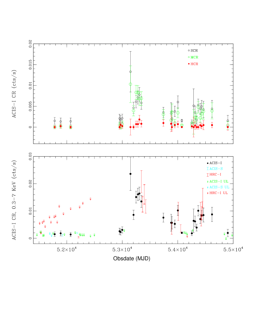
Figure 2: Light curve for r1-25. Top Panel: Count Rate in the Soft (0.3-1.1 keV), Medium (1.1-2 keV), and Hard (2-7 keV) bands vs. Obsdate. Bottom Panel: Total count rate in ACIS-I units (in the energy range of 0.3-7 keV) vs. Obsdate. See text for how we converted ACIS-S and HRC-I observations to ACIS-I units.

Table 1 shows the photometry results for r1-25. Columns 4, 5, and 6 show the Soft, Medium, and Hard count rates, respectively. The uncertainties are 1$\sigma$ in size and calculated using Poisson statistics. Figure 2 shows the light curve for r1-25. The top panel shows the count rate in each band (soft, medium, and hard) vs. obsdate for the ACIS-I detections; it demonstrates that the relative count rates change over time for the source. The bottom panel of Figure 2 shows the total count rate in the ACIS-I band vs. obsdate. We used the pimms (Mukai, 1993) to convert ACIS-S and HRC-I count rates to ACIS-I units. We choose ACIS-I units because most of the detections of the source were in this instrument. We indicate ACIS-S and HRC-I observations as a range of values, and assumed N_H = 1.1 $\times$ $10^{21}$ cm^-2 for the conversion. For OBSID 1854, we assumed a thermal blackbody model with temperatures of 75 and 83 eV to determine the lower and upper limits of the range, respectively. For OBSID 1575, we used $k\,T$ = 120 eV and $k\,T$ = 150 eV to determine the range with the same column. For HRC-I detections and upper limits, as well as ACIS-S upper limits, we converted to ACIS-I units using $k\,T$ = 75 eV and $k\,T$ = 300 eV.

3 Evidence for State Change

We used the CIAO tool dmextract to create source spectra for all observations where more than 60 source counts were collected. Source spectra were extracted from a circular region with radius 6 pixels centered on the source. Associated background spectra were extracted from an annular region (also centered on the source) with inner and outer radii of 10 and 25 pixels, respectively. For all observations, we created spectral response files using the CIAO tasks mkacisrmf and mkarf (Fruscione et al., 2006).

We modeled the resulting spectra using the XSPEC package (Arnaud, 1996). Since the number of source counts is small, we fit the spectra (binned to have one count per bin, as suggested in the XSPEC documentation) using the C-statistic (Cash, 1979) rather than the $\chi^{2}$ statistic, which has been shown to introduce a systematic bias in parameter estimation in low count rate spectra. The C-statistic as implemented in Xspec models the source and background spectrum simultaneously, scaling the background spectrum channel by channel to the size of the source region . One $\sigma$ uncertainties were estimated using the error command. We found that model fits to observations with less than 60 counts were not constrained; for this reason, we do not include them in our spectral analysis of r1-25. The four Obs-IDs with more than 60 counts were: 1575 (ACIS-S, 183 source counts), 4720 (ACIS-I, 61 source counts), 4721 (ACIS-I, 65 source counts) and 4722 (ACIS-I, 62 source counts).

We fit a simple absorbed blackbody model to each spectrum in the energy range 0.3-8.0 keV, using the wabs model for the interstellar absorption (Morrison & McCammon, 1983). None of the spectra had enough counts below 1 keV to place a tight constraint on the interstellar column density (in several cases the fits were consistent with no absorption), so we fixed N_H at two values representative of the range expected towards an X-ray source in M31 (1.1 $\times$ 10²¹ and 6.4 $\times$ 10²¹ cm^-2). The lower limit was taken from Di Stefano et al. (2004). The upper limit is shown for completeness; it is very unlikely that the source has such a large column density. The resulting parameter values and their 1 $\sigma$ uncertainties are presented in Table 2. We note that our results for ObsID 1575 (we found 0.110 keV $\leq$ $k\,T$ $\leq$ 0.130 keV) are consistent with those reported in Di Stefano et al. (2004) (they found that $k\,T$ = 0.122 keV). Examining the temperatures found for r1-25, a clear increase in the later observations can be seen, independent of the choice of absorbing column. Furthermore, r1-25 significantly changes in luminosity when it changes state. At the 90% confidence level, the temperature found for the ACIS-S spectrum is $\sim$0.1 keV lower than the ACIS-I values. The blackbody temperature returned by the model fitting is constrained primarily by the high energy cut off. Although ACIS-I has poorer low energy sensitivity, the fact that significantly harder counts are detected in such short exposures indicates that the increase in model temperature is real and independent of the differences between the two ACIS instruments.

4 Optical Observations and Analysis

The location of r1-25 has been observed with the ACS camera onboard HST. The source has been observed 4 times: on 2004-01-23 (observation j8vp03010) for 2200 seconds, 2004-08-15 (observation j8vp05010) for 2200 seconds, 2006-02-10 (observation j9ju01010) for 4360 seconds, and 2007-01-10 ( observation j9ju06010) for 4672 seconds. Images are only available in the F435W filter (approximately equal to the B filter in ground based systems). Only one Chandra observation (ObsID 8183) was taken within a week of an ACS observation (j9ju06010) of the source. However, the source was not detected in ObsID 8183.

All data were obtained using the Wide Field Channel (WFC), which has a $202\arcsec$ $\times$ $202\arcsec$ field of view (Maybhate et al., 2010). Each observation was carried out in the standard four pointing dither pattern (Maybhate et al., 2010). These individual images were then combined using the PyRAF task MultiDrizzle (Fruchter et al., 2009), which also removes cosmic rays and corrects the geometrical distortion which results from the orientation of the ACS with respect to the HST focal plane. We chose not to apply an automatic background subtraction in order to perform photometry, since there is a steep gradient in the diffuse light this close to the center of M31 making background estimation unreliable. Finally, we utilized the ability of MultiDrizzle to resample the spatial scale of the image, resulting in a final pixel scale of $0.025\arcsec$/pix.

The World Coordinate System (WCS) in HST images can be offset from standard reference frames by as much as one arcsecond (Maybhate et al., 2010). To improve the astrometry, we registered the final drizzled images to the WCS of the Local Group Survey (LGS) images of M31 (Massey et al., 2006). Stars common to both images were identified, and their centroid positions calculated using the IRAF task imcentroid. We then used the task ccmap in IRAF to update the WCS of the HST images. The final rms (1$\sigma$) errors in the alignment were of order 0.006$\arcsec$ in RA, and 0.002$\arcsec$ in declination. We note that the RMS errors on the alignment of the HST images to the WCS of the LGS survey were always smaller than 0.01$\arcsec$ (which is smaller than one pixel in the rescaled images).

We also aligned the deepest Chandra observation (ObsID 1575) with the WCS of the LGS images using the same procedure applied to the HST images. We found an alignment error of 0.109$\arcsec$ in RA and 0.149$\arcsec$ in DEC. The centroid position in the corrected WCS for the source is RA:00:42:47.90, DEC:+41:15:49.99, with errors of 0.08$\arcsec$ (RA) and 0.07$\arcsec$ (DEC). To get the final positional error, we added the alignment and centroid errors in quadrature. The final RA error is 0.13$\arcsec$ and final DEC error is 0.17$\arcsec$ (these are 1$\sigma$ errors).

Since the WFC images cover such a large area and contain so many stars, we extracted subimages 1000 pixels on a side centered on our source of interest and performed photometry on those. We used the DAOPHOT II and ALLSTAR routines (Stetson et al., 1990) to find and photometer stars in the images. Stars suitable for calculating a point spread functions (PSFs) were identified by hand to avoid problems due to crowding. The final measured counts for each star were converted first to count rate by dividing by the exposure time of each observation, and then to AB system magnitudes using the conversion factors in the ACS users handbook (Maybhate et al., 2010).

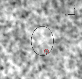
Figure 3: HST ACS images of the location of r1-25, obtained in the F435W filter on four separate dates. Top Left: Observation j8vp03010, Top Right: observation j8vp05010, Bottom Left: Observation j9ju01010, Bottom Right: Observation j9ju06010. Each image is 3$\arcsec$ on a side. The black ellipse denotes the 3$\sigma$ X-ray positional error ellipse of r1-25. The ellipse has a semi-major axis (3$\sigma$ RA error) = 0.39$\arcsec$ and a semi-minor axis (3$\sigma$ DEC error) = 0.51 $\arcsec$. The red circle shows the only consistently detected, resolved source found by DAOphot.

We show the final reduced image for the source in Figure 3, superimposed with the X-ray 3$\sigma$ positional error ellipse. The ellipse is drawn using the 3$\sigma$ RA error (0.39$\arcsec$) as the semi-major axis and the 3$\sigma$ DEC error (0.51$\arcsec$) as the semi-minor axis. The location of r1-25 is extremely crowded, and being so close to the core is subject to a high background of diffuse light. In our series of four images, two (j9ju01010 and j9ju06010) are also significantly deeper, which affects the completeness of the stars we can detect. The small size of the Chandra error circle does however simplify the analysis of the photometry, since very few sources are inside the X-ray 3$\sigma$ error ellipse. Examining the images, a number of sources are detected inside the error circle, although most are unresolved. We note that there are no catalog stars within the Chandra error ellipse. In fact, only one source is resolved inside the error ellipse in all four images by the photometry source detection algorithm. We have marked this source with a red circle in Figure 3.

The single resolved source in Figure 3 has observed magnitudes of 24.45 $\pm$ 0.06, 24.27 $\pm$ 0.05, 24.31 $\pm$ 0.04 and 24.41 $\pm$ 0.04 in each of the four images, where the uncertainties are 1$\sigma$ in size. Using the standard $E(B-V)=0.062$ for M31 (Schlegel et al., 1998), the extinction in the F435W filter is 0.785 magnitudes. Thus, the star’s $M_{B}$ is between -0.80 and -0.98 in the four observations, assuming $(m-M)_{0}$ = 24.47 (Holland, 1998). This demonstrates that, within the uncertainties, there is no evidence of variability in this object. Although other sources are picked up by the DAOphot detection algorithm inside the error ellipse in some images, these additional detections can be accounted for by the longer exposure time, or are unreliable due to crowding.

Grupe et al. (2010) looked at the spectral energy distribution of 92 active galactic nuclei that had soft X-ray spectra. The AGN they studied had comparable X-ray count rates to r1-25. However, the AGN were much brighter in the B band (14 $<$ $m_{B}$ $<$ 18 ) than any source in Figure 3. For this reason, we are confident that r1-25 is not an AGN.

With no color information, we cannot determine what the object marked in Figure 3 is for certain. If it is a star, it would correspond to a late B type with bolometric luminosity of $~{}10^{36}$ ergs s^-1. We note that it is too luminous in the B band to be a red giant, and too dim to be a red supergiant.

5 Models

The state changes observed in r1-25 are extremely unusual for an SSS. In this section, we consider a number of physical models with the goal of uncovering the nature of the X-ray emitting source. In order for any model of r1-25 to be successful, it must be able to explain all of the observed features of the source. These features include the source’s appearance as an SSS-HR source in observation 1575 with ACIS-S, with kT $\sim$ 130 eV and a 0.3–8 keV luminosity of 4 $\times$ 10³⁶ erg s^-1. We wish to emphasize once again that even though r1-25 had an effective temperature in excess of 100 eV when detected as an SSS (much higher than most SSSs), it satisfied the strictest SSS criterion as defined in Di Stefano et al. (2004). That is, the detection in observation 1575 (when the source was an SSS) had no hard counts, medium counts consistent with zero, and at least 3$\sigma$ detection in the soft band.

Furthermore, the model must explain the subsequent detections of the source as a $\sim$250 eV source, with higher luminosity than in the soft state ($\sim$10³⁷ erg s^-1). Lastly, the model must be consistent with an optical counterpart with F435W magnitude fainter than $\sim$24.3 ($M_{B}$ fainter than $\sim$ -1). We note that white dwarf, neutron star, and black hole SSSs are consistent with this optical constraint. The following subsections outline white dwarf, neutron star and black hole models, and compare their features to the observed properties of r1-25.

5.1 White Dwarfs

White dwarfs that have recently experienced novae have temperatures and luminosities that can make them detectable as SSSs. Many SSSs detected in M31 were recent novae (e.g., Pietsch et al., 2005, 2007; Stiele et al., 2010, references therein). When the white dwarf cools, some novae are detected as harder X-ray sources, but the X-ray luminosity is around $10^{32}-10^{33}$ ergs s^-1 (Sala et al., 2010). In contrast, novae in a supersoft state are detected with $k\,T$ $\sim$ 50 eV and L_X of $10^{37}-10^{38}$ ergs s^-1 (e.g., Stiele et al., 2010, references therein). Thus r1-25, even in its softest state (with kT $\sim$130 eV and L_X of 4 $\times$ 10³⁶ erg s^-1), is too hard to be consistent with the very soft emission detected in typical supersoft novae. Also, the source is not consistent with the harder states of novae. That is r1-25 in its hardest state ($\sim$250 eV and L_X of 1.1 $\times$ 10³⁷ erg s^-1) is softer and more luminous than novae in their hard states. Moreover, unlike novae, the harder states of r1-25 are more luminous than its soft state. We therefore turn to models in which a white dwarf accretes matter at high rates.

When a white dwarf accretes mass at a high enough rate that the incoming matter can experience nuclear burning, the white dwarf can appear as an SSS. In this case, the source will not be in a hard state. The copious energy we receive from such sources is provided by nuclear burning, rather than accretion. The effective radii are comparable to the white dwarf radii, so the emission can be characterized by values of $k\,T$ in the range of tens of eV for low-mass white dwarfs, and $\sim 100$ eV for white dwarfs approaching the Chandrasekhar mass ($M_{C}$). For each white dwarf mass, nuclear burning can occur only within a narrow range of accretion rates (Nomoto, 1982; Iben, 1982; Fujimoto, 1982; Shen & Bildsten, 2008, references therein). These rates are very high: $\sim 10^{-7}M_{\odot}$ for a solar-mass white dwarf, ten times higher for a white dwarf with mass near $M_{C}$ (Di Stefano, 2010). At such rates of infall, accretion alone produces luminosities in the range of $10^{36}-10^{37}$ ergs s^-1, typically a few percent of the total energy of the system.

Consider a case, when its accretion rate places a white dwarf near the lower end of the steady-burning region, or just below it. In this case, nuclear burning may be episodic. During and just after nuclear-burning episodes, the emission is dominated by soft emission. As the white dwarf cools, however, it becomes less luminous and the emission is dominated by accretion. Although at high rates of accretion, the emission is expected to be softer than typical for low-accretion-rate white dwarfs, such as cataclysmic variables, it can nevertheless be harder than typical of SSSs (e.g., Popham & Narayan, 1995; Patterson & Raymond, 1985). Thus, the source could appear to be quasisoft or hard. If the donor is a giant or a Roche-lobe filling star in a circular orbit, the accretion rate should could continue to be high. The source will continue to be detected as a harder source. Nuclear burning episodes occurring at intervals ranging from months to decades would make the source more luminous and detectable as an SSS.

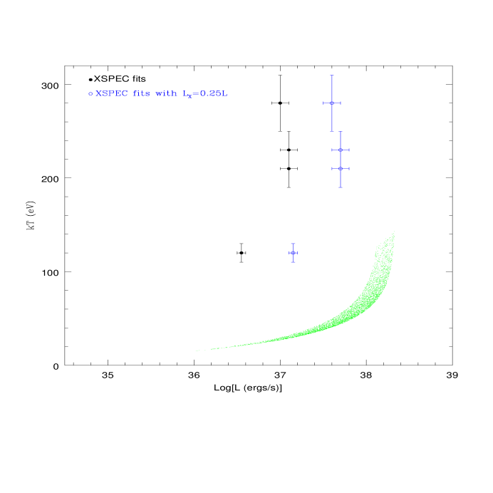
Figure 4: Plot of $k\,T$ vs. the logarithm of the bolometric luminosity, LOG[L]. The black and blue points show the observations with XSPEC fits from Table 2 (assuming N_H = 1 $\times$ $10^{21}$ cm^-2). The solid black points represent XSPEC fits assuming L_X = L, and the open blue points assume L_X = $0.25L$. The green points represent the $k\,T$ and LOG[L] for various quasi-steady nuclear burning white dwarfs.

The points made above about the quasi-steady nuclear burning white dwarf model are illustrated in Figure 4. The figure is a plot of $k\,T$ vs. the logarithm of bolometric luminosity, LOG[L] for various quasi-steady nuclear burning white dwarfs (green points) along with the r1-25 spectra (black and blue points). The points represent the XSPEC spectral fits of r1-25 shown in Table 2. The solid black points represent the fits where we assume L_X = L. The X-ray luminosity, however, is not equivalent to the bolometric luminosity. We assume that the X-ray luminosity represents, at least a quarter of the bolometric luminosity. Thus, we plot the open blue circles which represent XSPEC fits assuming L_X = $0.25L$. The plot clearly indicates that the quasi-steady nuclear burning white dwarf model does not fit r1-25, as the data are too hard and/or dim to fit the model. That is, none of the XSPEC points fall in the range of quasi-steady nuclear burning white dwarf.

5.2 Neutron Stars

Isolated neutron stars and neutron stars in quiescent low-mass X-ray binaries (qLMXBs) have been observed with spectra in the SSS or QSS range, but they are typically 3-5 orders of magnitude less luminous than the “classical” SSSs and QSSs (e.g., Haberl, 2007; Pires et al., 2009). Neutron stars accreting at high rates, however, have luminosities in the range (above $10^{36}$ erg s^-1) observed for SSSs and QSSs. But, at the time SSSs were discovered, all known accreting neutron stars emitted hard x-rays. The lack of hard emission from SSSs therefore seemed to be more easily accommodated in white dwarf models.

Nevertheless, Kylafis & Xilouris (1993) showed that accreting neutron stars can be observed as SSSs under the right circumstances. They considered near-Eddington accretion through a disk. Radiation pressure from the inner disk can push some plasma into an “extensive outer disk corona.” If the corona extends to large enough radii, and if it is optically thick, the neutron star will radiate as an SSS. Indeed, there is observational support for the idea that neutron stars can produce very soft spectra. For example, Hughes (1994) discovered a transient pulsar in the Small Magellanic Cloud that has an unpulsed, highly luminous (near Eddington) soft $\sim 35$ eV component. If such a system were to be viewed from an angle at which the hard radiation is not detected, it would have the properties associated with the “classical” SSSs first discovered in the Magellanic Clouds (Long et al., 1981).

Although the details of the model considered by Kylafis & Xilouris (1993) may not apply to all systems, their work, combined with observations, indicates that neutron star models must be considered. Yet, beyond the success of the white-dwarf models, there is another reason that neutron star models have not been popular, and that was alluded to by Kylafis & Xilouris (1993). This can be simply stated by saying that the physics determining the size of the photosphere was put in by hand. Thus, the solutions for radial flows that extend out to at least a few thousand neutron star radii produce SSS-like behavior, and radial flows that extend out to at most a few hundred neutron star radii produce more standard LMXB-like behavior. The range of photospheric radii between these two extremes would be associated with luminous emitters of thermal radiation with $k\,T$ in the range between roughly $100$ eV and a few hundred eV; that is, the sources would be QSSs, which had not yet been discovered.

Here we point out that the discovery of QSSs provides reasons to revisit neutron star models, eliminating the need for fine tuning problem that Kylafis & Xilouris (1993) encountered. The key issue to address is what determines the size of the photosphere. It is likely to be linked to accretion rate, with higher rates capable of producing larger photospheres, as in the Kylafis & Xilouris (1993) model. Here we suggest that in some cases, the edge of the magnetosphere could roughly correspond to the photosphere. If this is the case, then, given that the mass, radius, and magnetic field of the accretor are all roughly constant over time scales of months to years, the photospheric radius would be driven primarily by changes in the accretion rate. Equation (1) and Figure 5 show the relationship that would be predicted between the temperature and luminosity.

Consider a neutron star producing near-Eddington soft emission. If this emission emanates from a nearly spherical photosphere with radius equal to the Alfven radius, then

$$k\,T=100.4\,{\rm eV}\,\Bigg{(}\frac{10^{11}{\rm G}}{B_{s}}\Bigg{)}^{\frac{2}{7}}\Bigg{(}\frac{10\,{\rm km}}{R_{NS}}\Bigg{)}^{\frac{5}{7}}\Bigg{(}\frac{M_{\odot}}{M}\Bigg{)}^{\frac{1}{14}}\Bigg{(}\frac{L}{10^{37}{\rm ergs\,s}^{-1}}\Bigg{)}^{\frac{11}{28}}$$ (1)

In this expression, $R_{NS}$ is the radius of the neutron star, $B_{s}$ is the value of magnetic field on the surface, and $M$ and $L$ represent the neutron star’s mass and luminosity, respectively. We derive this expression from equation 11 in Ostriker & Davidson (1973). An interesting feature of this expression is that there are ranges of reasonable values of the physical parameters in which the $k\,T$ is in the range expected for SSSs or QSSs. Furthermore, for a specific neutron star, the effective temperature depends on L which can change as the accretion rate changes. Since changes in accretion rate are common, we may therefore expect the effective temperatures of some neutron stars to change. Depending on the physical parameters, these changes could produce transitions from SSS to QSS states.

Figure 5 shows two plots of $k\,T$ vs. LOG[L]. The top panel shows several curves which differ from each other in the value of $B_{s}$, which changes by a factor of ten between curves, as shown. The bottom plot shows the r1-25 spectra along with the $B_{s}=10^{10}$ G curve. The black points represent the XSPEC fits shown in Table 2. The plots were made in the same manner as in Figure 4 (see $\S$5.1), except that we assumed neutron star models have L $\approx$ L_X. Figure 5 shows that the distribution of points is roughly consistent with what is expected for the neutron star model discussed above. The XSPEC points seem to follow the same trend as the curve, with some variation.

The general agreement between the trend of increasing $k\,T$ with increasing luminosity is promising, and neutron-star models in which the photospheric radius is not governed by the size of the Alfven radius may follow similar trends, with $k\,T$ increasing with luminosity. Nevertheless, this general trend is not unique to neutron star models, as we will see in §5.3, where black hole models are considered. It is therefore important to develop observational criteria that can identify the nature of the compact accretor.

For example, the neutron-star natures of LMXBs in the Galaxy’s globular clusters have been verified through the detections of both bursts (e.g., Lewin et al., 1993) and pulsed (e.g., Zhelezniakov, 1981) radiation. Both types of variable components are expected to be harder than the dominant softer radiation from an extended photosphere. Thus, for example in an x-ray pulsar, the diagnostic for the neutron star model would be periodicity in the arrival times of the harder photons. If, therefore, we can identify QSSs and state changers in the Milky Way or in the Magellanic Clouds, we can test models by searching for evidence of hard bursts or pulses. Detecting these in state changers, or in QSSs, would be possible if the system is close enough, and would verify the neutron-star nature of the accretor.

5.3 Black Holes

Accreting black holes can exhibit thermal-dominant states in which the emission is dominated by a component emanating from the inner portion of the accretion disk (e.g., Remillard & McClintock, 2006). SSSs and QSSs have therefore both been suggested as possible black holes. In fact, the most well-known state changer is M101-ULX-1, an ultraluminous SSS that has been detected also in high QSS and low-hard states (e.g., Kong et al., 2004; Kong & Di Stefano, 2005; Mukai et al., 2005). M101-ULX-1 is almost certainly a black hole. Its mass could be either in the range typical of Galactic stellar-mass black holes or else in the higher range ($50-10^{4}\,M_{\odot}$) suggested for intermediate-mass black holes.

The luminosity of r1-25 is 1-3 orders of magnitude smaller than the luminosities measured for M101-ULS-1 when it is in a soft state. It is therefore highly unlikely to be an intermediate-mass black hole. In fact, if the luminosity is less than roughly a percent of the Eddington luminosity, then the inner disk will not be optically thick and the emission will not be thermal. This suggests that, if this source is a black hole, it is more likely to be of stellar mass. The top panel of Figure 7, first shown in Di Stefano et al. (2010), shows that QSS emission is expected in the thermal-dominant state of black holes with mass below $\sim 100\,M_{\odot}.$ The radius of the inner disk would determine the value of the effective temperatures; the spectrum could be either QSS or SSS. At lower rates of accretion, the emission would be hard. Note that there are two curves for each mass; the top curve assumes the inner portion of the accretion disk is at 6MG/c² (3r_s, where r_s is the Schwarzschild radius) and the bottom assumes 18MG/c² (9r_s). Note that that the top curve (at 3r_s) represents the maximum luminosity and temperature for this model in which the radiation comes from the inner disk.

Figure 6 shows the r1-25 spectra along with the 10$M_{\odot}$ and 100$M_{\odot}$ curves. The black points representing the XSPEC fits shown in Table 2 were plotted in the same manner as in Figure 5 (see $\S$5.2). The distribution of the points with XSPEC fits is roughly consistent with what is expected for a black hole of roughly 10$M_{\odot}$.

6 Conclusion

We have tracked the long-term behavior of the M31 X-ray source r1-25. First observed by ROSAT on 1990-07-24, then by both Chandra and XMM-Newtonand most recently by Swift, r1-25 is one of the best-studies soft X-ray sources. There are 86 public Chandra observations of the source through June 2, 2009, with 45 detections. For XMM-Newton, there are 26 public observations of the source, with Stiele et al. (2010) reporting detections in only the 2004 data. The detections of the source start in 1999 and continue through 2009.

By doing this we have documented the fact that r1-25 has transitioned from an SSS to a harder, QSS state. In the SSS state its estimated X-ray luminosity is a few times $10^{36}$ ergs $s^{-1}$, and the luminosity appears to be higher, but not much over $10^{37}$ ergs $s^{-1}$ in the harder state. Only one other X-ray source, M101-ULX-1, has well-studied state changes (e.g., Kong et al., 2004; Kong & Di Stefano, 2005; Mukai et al., 2005). While M101-ULX-1, which has been observed with X-ray luminosity as high as $10^{40}-10^{41}$ ergs $s^{-1}$, is almost certainly a black hole, the nature of r1-25 is more difficult to establish, because its luminosity range is consistent with white dwarf, neutron star, or black hole accretors.

Whatever its nature, its behavior is different from anything we have observed. We have shown that the observed behavior is consistent with a black hole accretor with a mass in the 10$M_{\odot}$ range. In this case, our observations of r1-25 have all found it to be in a thermal-dominant state. The inner disk radius would have been larger in the SSS state. If r1-25 is a black hole with a mass of approximately $10M_{\odot},$ it could be more luminous in future observations, if the donor star is able to contribute mass at a higher rate. Should the luminosity approach the Eddington luminosity, the system would be unlikely to remain in the thermal dominant state, and hard emission could be detected. Similarly, if the luminosity falls below $\sim 1\%$ of the Eddington value, the spectrum would likely be hard.

We have also shown that the observed behavior of r1-25 is consistent with a neutron star accretor with $B_{s}$ = $10^{10}$ G. We assume that the magnetic field should be constant over the short interval of observations of the source. The model suggests that the harder states are more luminous than the softer ones, which is consistent with the r1-25 spectra. We note that neutron star models are testable if we can find state changers and QSSs in the Milky Way or Magellanic Clouds, as both bursts and pulsed radiation would be detectable in nearby neutron stars.

White dwarf models are the least likely fit for r1-25. The source does not seem to exhibit behavior of a post-nova system, as its spectrum is harder than novae that are SSSs (even when r1-25 is in its soft state). The source is also too luminous and soft to be consistent with novae in their harder states. Furthermore, quasi-steady nuclear burning white dwarf models do not fit the data. We have shown that quasi-steady nuclear burning models can produce both supersoft and quasisoft radiation, but the model is too soft and/or luminous to fit the r1-25 spectra.

We note that there are other state-changing sources in external galaxies. For example, there are nine state changing sources in nearby spiral galaxy M33. If we study a large enough sample of state-changers, we are likely to find examples of all three (white dwarf, neutron star, and black hole) models. Continued monitoring of these sources will play an important role in testing these models. It is also important to identify QSSs and state-changers in the Magellanic Clouds and Galaxy, where many test of the nature of the accretors can be conducted.

Figure 1: Source (solid) and background (dashed) apertures for r1-25, displayed on a $\sim$432 kilosecond merged Chandra HRC-I observation of M31.

Figure 5: Plot of $k\,T$ versus $L$ for the neutron star model described by Equation 1. Top Panel: Each curve corresponds to a fixed value of the magnetic field on the surface of the neutron star; $B_{s}$ changes by a factor of ten between curves. Since the field is not expected to vary this much over short times, the system should evolve along the curves. Thus, if the luminosity increases or decreases, so does the temperature. Bottom Panel: The $B_{s}=10^{10}$ G curve is plotted with the r1-25 spectra. The black points represent XSPEC fits from Table 2 (assuming N_H = 1 $\times$ $10^{21}$ cm^-2).

Figure 6: Figure taken from Di Stefano et al. (2010). It is a plot of $k\,T$ versus LOG[L] for the inner portion of the accretion disk around black holes. Each pair of two curves of a single color corresponds to a fixed black hole mass which labels the regions between the curves. The upper curve of each color corresponds to a disk with inner radius $6M_{BH}G/c^{2}$ (3r_s), while the lower curve corresponds to an inner disk with 9r_s. The point at the bottom (top) of each curve corresponds to the luminosity of the inner disk being $1\%L_{Eddington}$ ($10\%L_{Eddington}$). The curves are plotted with the r1-25 spectra. The black points represent the XSPEC fits from Table 2 (assuming N_H = 1.1 $\times$ $10^{21}$ cm^-2)

Table 1: Photometry for r1-25

		Exposure Time	SCR	MCR	HCR	TCR	Total
ObsID	OBSMJD	seconds	$10^{-3}$s-1	$10^{-3}$s-1	$10^{-3}$s-1	$10^{-3}$s-1	Counts
ACIS-I Observations
312	51783.8	4666	1.5 $\pm$ 0.8	0.0 $\pm$ 0.4	0.0 $\pm$ 0.4	1.5 $\pm$ 0.8	7 $\pm$ 4
1581	51891.1	4404	1.3 $\pm$ 0.8	0.2 $\pm$ 0.5	0.2 $\pm$ 0.5	1.8 $\pm$ 0.9	8 $\pm$ 4
1583	52070.8	4903	1.4 $\pm$ 0.8	0.0 $\pm$ 0.4	0.0 $\pm$ 0.4	1.4 $\pm$ 0.8	7 $\pm$ 4
4678	52952.3	3894	2.1 $\pm$ 1.0	0.5 $\pm$ 0.7	0.0 $\pm$ 0.5	2.6 $\pm$ 1.1	10 $\pm$ 4
4679	52969.9	3820	1.8 $\pm$ 1.0	0.0 $\pm$ 0.5	0.5 $\pm$ 0.7	2.3 $\pm$ 1.1	9 $\pm$ 4
4680	53000.3	4198	2.1 $\pm$ 1.0	0.7 $\pm$ 0.7	0.2 $\pm$ 0.6	3.1 $\pm$ 1.1	13 $\pm$ 5
4682	53148.7	3945	13.3 $\pm$ 4.9	10.3 $\pm$ 4.4	0.0 $\pm$ 1.9	23.6 $\pm$ 6.1	23 $\pm$ 6
4719	53203.9	4123	4.6 $\pm$ 1.4	3.9 $\pm$ 1.3	0.0 $\pm$ 0.5	8.6 $\pm$ 1.7	35 $\pm$ 7
4720	53250.6	4108	6.1 $\pm$ 1.5	8.3 $\pm$ 1.7	0.7 $\pm$ 0.7	15.1 $\pm$ 2.2	62 $\pm$ 9
4721	53282.9	4132	7.1 $\pm$ 1.6	8.3 $\pm$ 1.7	0.7 $\pm$ 0.7	16.1 $\pm$ 2.2	66 $\pm$ 9
4722	53309.1	3894	7.8 $\pm$ 1.7	6.8 $\pm$ 1.6	1.8 $\pm$ 1.0	16.4 $\pm$ 2.3	63 $\pm$ 9
4723	53344.4	4035	5.8 $\pm$ 1.5	6.9 $\pm$ 1.6	0.8 $\pm$ 0.8	13.5 $\pm$ 2.2	51 $\pm$ 8
7136	53741.8	3991	3.5 $\pm$ 1.2	3.0 $\pm$ 1.2	1.0 $\pm$ 0.8	7.6 $\pm$ 1.7	30 $\pm$ 7
7137	53881.2	3952	3.3 $\pm$ 2.6	1.6 $\pm$ 2.2	0.8 $\pm$ 1.9	5.7 $\pm$ 3.1	7 $\pm$ 4
7138	53895.7	4107	2.1 $\pm$ 1.6	3.6 $\pm$ 1.9	0.0 $\pm$ 1.0	5.7 $\pm$ 2.3	11 $\pm$ 4
7139	53947.0	3987	3.8 $\pm$ 1.2	1.0 $\pm$ 0.8	0.5 $\pm$ 0.7	5.3 $\pm$ 1.4	21 $\pm$ 6
7140	54002.8	4117	6.0 $\pm$ 1.5	3.4 $\pm$ 1.2	0.7 $\pm$ 0.7	10.2 $\pm$ 1.9	42 $\pm$ 8
7064	54073.9	23238	1.5 $\pm$ 0.3	0.5 $\pm$ 0.2	0.0 $\pm$ 0.1	2.0 $\pm$ 0.3	46 $\pm$ 8
7068	54253.9	7693	1.0 $\pm$ 0.7	0.6 $\pm$ 0.6	0.2 $\pm$ 0.5	1.8 $\pm$ 0.8	9 $\pm$ 4
8192	54286.5	4073	5.1 $\pm$ 4.1	1.28 $\pm$ 3.0	0.0 $\pm$ 2.4	6.4 $\pm$ 4.4	5 $\pm$ 3
8193	54312.1	4129	3.5 $\pm$ 1.6	2.3 $\pm$ 1.4	0.4 $\pm$ 0.9	6.2 $\pm$ 2.0	16 $\pm$ 5
8194	54340.5	4033	1.7 $\pm$ 0.9	2.2 $\pm$ 1.0	0.0 $\pm$ 0.5	3.9 $\pm$ 1.3	16 $\pm$ 5
8195	54369.6	3965	5.3 $\pm$ 1.4	4.8 $\pm$ 1.4	0.0 $\pm$ 0.5	10.1 $\pm$ 1.9	40 $\pm$ 7
8186	54407.2	4134	4.4 $\pm$ 1.3	2.2 $\pm$ 1.0	0.5 $\pm$ 0.7	7.0 $\pm$ 1.6	29 $\pm$ 6
8187	54431.2	3837	5.0 $\pm$ 1.4	3.2 $\pm$ 1.2	0.2 $\pm$ 0.6	8.3 $\pm$ 1.8	32 $\pm$ 7
9520	54463.7	3962	4.2 $\pm$ 2.0	3.8 $\pm$ 1.9	0.5 $\pm$ 1.1	8.5 $\pm$ 2.6	18 $\pm$ 5
9529	54617.5	4113	4.4 $\pm$ 2.0	3.9 $\pm$ 1.9	0.5 $\pm$ 0.7	8.8 $\pm$ 2.6	18 $\pm$ 5
10553	54901.6	4104	1.6 $\pm$ 1.3	0.4 $\pm$ 0.9	0.0 $\pm$ 0.7	2.0 $\pm$ 1.3	5 $\pm$ 3
ACIS-S Observations
1854	51922.4	4694	4.3 $\pm$ 1.2	0.7 $\pm$ 0.6	0.0 $\pm$ 0.4	4.9 $\pm$ 1.3	23 $\pm$ 6
1575	52187.0	37664	4.6 $\pm$ 0.4	0.4 $\pm$ 0.1	0.0 $\pm$ 0.1	4.9 $\pm$ 0.4	184 $\pm$ 15
HRC-I Observations
1912	52214.0	46732	$\cdots$	$\cdots$	$\cdots$	0.5 $\pm$ 0.1	21 $\pm$ 6
5925	53345.8	46311	$\cdots$	$\cdots$	$\cdots$	14.6 $\pm$ 0.6	678 $\pm$ 28
6177	53366.3	20038	$\cdots$	$\cdots$	$\cdots$	8.8 $\pm$ 0.7	176 $\pm$ 13
5926	53366.8	28268	$\cdots$	$\cdots$	$\cdots$	8.7 $\pm$ 0.6	246 $\pm$ 16
6202	53398.1	18046	$\cdots$	$\cdots$	$\cdots$	11.3 $\pm$ 0.8	204 $\pm$ 14
5927	53398.8	27000	$\cdots$	$\cdots$	$\cdots$	11.4 $\pm$ 0.7	308 $\pm$ 18
5928	53422.7	44856	$\cdots$	$\cdots$	$\cdots$	8.2 $\pm$ 0.4	369 $\pm$ 20
7283	53891.3	19942	$\cdots$	$\cdots$	$\cdots$	3.4 $\pm$ 0.4	67 $\pm$ 9
7284	54008.9	20002	$\cdots$	$\cdots$	$\cdots$	10.6 $\pm$ 0.7	212 $\pm$ 14
7285	54052.3	18517	$\cdots$	$\cdots$	$\cdots$	3.8 $\pm$ 0.5	70 $\pm$ 9
8526	54411.6	19944	$\cdots$	$\cdots$	$\cdots$	9.6 $\pm$ 0.7	191 $\pm$ 14
8527	54421.8	19981	$\cdots$	$\cdots$	$\cdots$	6.3 $\pm$ 0.6	126 $\pm$ 12
8528	54432.8	19975	$\cdots$	$\cdots$	$\cdots$	7.7 $\pm$ 0.6	154 $\pm$ 13
8529	54441.6	18923	$\cdots$	$\cdots$	$\cdots$	8.9 $\pm$ 0.7	168 $\pm$ 13
8530	54451.5	19915	$\cdots$	$\cdots$	$\cdots$	12.4 $\pm$ 0.8	247 $\pm$ 16

Note. — Columns 4, 5, and 6 are the count rates in the Soft (0.3-1.1 keV), Medium (1.1-2 keV), Hard (2-7 keV) bands, respectively. All rates are corrected by a vignetting factor.

Table 2: Spectral Fitting Results

	NH = 1.1 $\times$ $10^{21}$ cm-2				NH = 6.4 $\times$ $10^{21}$ cm-2
Obs ID	$k\,T$ (keV)	Normalization (10-6)	LX (1037 ergs s-1)		$k\,T$ (keV)	Normalization (10-6)	LX (1037 ergs s-1)
1575	0.12 $\pm$ 0.01	0.73${}^{+0.09}_{-0.08}$	0.40		0.065 $\pm$ 0.003	160${}^{+50}_{-40}$	97
4720	0.28 $\pm$ 0.03	1.7 $\pm$ 0.3	1.0		0.19 $\pm$ 0.02	8${}^{+3}_{-2}$	4.8
4721	0.23 $\pm$ 0.02	2.0${}^{+0.4}_{-0.3}$	1.2		0.17 $\pm$ 0.01	10${}^{+4}_{-3}$	6.0
4722	0.21 $\pm$ 0.02	2.4${}^{+0.5}_{-0.4}$	1.4		0.11 $\pm$ 0.01	60${}^{+40}_{-20}$	36

Note. — Spectral fits were carried out in the energy range 0.3-8.0 keV, using a simple absorbed blackbody model (wabs model was used for absorption). Luminosities are given for the same energy range and are corrected for assumed absorption. All uncertainties are 1$\sigma$ in size.

References

- Arnaud (1996) Arnaud, K. A. 1996, Astronomical Data Analysis Software and Systems V, 101, 17
- Cash (1979) Cash, W. 1979, ApJ, 228, 939
- Di Stefano & Nelson (1996) Di Stefano, R., & Nelson, L. A. 1996, Supersoft X-Ray Sources, 472, 3
- Di Stefano & Kong (2003) Di Stefano, R., & Kong, A. K. H. 2003, arXiv:astro-ph/0311374
- Di Stefano et al. (2003) Di Stefano, R., Kong, A. K. H., VanDalfsen, M. L., et al. 2003, ApJ, 599, 1067
- Di Stefano et al. (2003) Di Stefano, R., Friedman, R., Kundu, A., & Kong, A. K. H. 2003, arXiv:astro-ph/0312391
- Di Stefano et al. (2004) Di Stefano, R., Kong, A. K. H., Greiner, J., Primini, F. A., Garcia, M. R. et al. 2004, ApJ, 610, 247
- Di Stefano & Kong (2004) Di Stefano, R., & Kong, A. K. H. 2004, ApJ, 609, 710
- Di Stefano et al. (2004) Di Stefano, R., Primini, F. A., Kong, A. K. H., & Russo, T. 2004, arXiv:astro-ph/0405238
- Di Stefano et al. (2006) Di Stefano, R., Kong, A., & Primini, F. A. 2006, arXiv:astro-ph/0606364
- Di Stefano (2010) Di Stefano, R. 2010, ApJ, 712, 728
- Di Stefano et al. (2010) Di Stefano, R., Kong, A., & Primini, F. A. 2010, New A Rev., 54, 72
- Di Stefano et al. (2010) Di Stefano, R., Primini, F. A., Liu, J., Kong, A., & Patel, B. 2010, Astronomische Nachrichten, 331, 205 B., Wachter, S., & Anderson, S. F. 1996, ApJ, 471, 979
- Freeman et al. (2002) Freeman, P. E., Kashyap, V., Rosner, R., & Lamb, D. Q. 2002, ApJS, 138, 185
- Fruchter et al. (2009) Fruchter, A. and Sosey, M. et al. 2009, “The MultiDrizzle Handbook”, Version 3.0 (Baltimore, STScI)
- Fruscione et al. (2006) Fruscione, A., McDowell, J. C., Allen, G. E., Davis, J. E., Durham, N. et al. 2006, Proc. SPIE, 6270
- Fujimoto (1982) Fujimoto, M. Y. 1982, ApJ, 257, 767
- Greiner (2000) Greiner, J. 2000, New Astronomy, 5, 137
- Greiner et al. (2004) Greiner, J., Di Stefano, R., Kong, A., & Primini, F. 2004, ApJ, 610, 261
- Grupe et al. (2010) Grupe, D., Komossa, S., Leighly, K. M., & Page, K. L. 2010, ApJS, 187, 64
- Haberl (2007) Haberl, F. 2007, Ap&SS, 308, 181
- Hachisu et al. (1996) Hachisu, I., Kato, M., & Nomoto, K. 1996, ApJ, 470, L97
- Holland (1998) Holland, S. 1998, AJ, 115, 1916
- Hughes (1994) Hughes, J. P. 1994, ApJ, 427, L25
- Iben (1982) Iben, I., Jr. 1982, ApJ, 259, 244
- Kaaret (2002) Kaaret, P. 2002, ApJ, 578, 114 Kerkwijk, M. H., & Anderson, J. 2007, ApJ, 660, 1428
- Kashyap et al. (2009) Kashyap, V., Primini, F. A., Glotfelty, K. J., Anderson, C. S., Bonaventura, N. R. et al. 2009, Bulletin of the American Astronomical Society, 41, 425
- Kong et al. (2002) Kong, A. K. H., Garcia, M. R., Primini, F. A., Murray, S. S., Di Stefano, R. et al. 2002, ApJ, 577, 738
- Kong et al. (2004) Kong, A. K. H., Di Stefano, R., & Yuan, F. 2004, ApJ, 617, L49
- Kong & Di Stefano (2005) Kong, A. K. H., & Di Stefano, R. 2005, ApJ, 632, L107
- Kong & Di Stefano (2003) Kong, A. K. H., & Di Stefano, R. 2003, ApJ, 590, L13
- Kylafis & Xilouris (1993) Kylafis, N. D., & Xilouris, E. M. 1993, A&A, 278, L43
- Lewin et al. (1993) Lewin, W. H. G., van Paradijs, J., & Taam, R. E. 1993, Space Science Reviews, 62, 223
- Liu & Di Stefano (2008) Liu, J., & Di Stefano, R. 2008, ApJ, 674, L73
- Liu (2011) Liu, J. 2011, ApJS, 192, 10
- Long et al. (1981) Long, K. S., Helfand, D. J., & Grabelsky, D. A. 1981, ApJ, 248, 925
- Massey et al. (2006) Massey, P., Olsen, K. A. G., Hodge, P. W., Strong, S. B., Jacoby, G. H. et al. 2006, AJ, 131, 2478
- Maybhate et al. (2010) Maybhate, A. et al. 2010, ”ACS Instrument Handbook”, Version 9.0
- Morrison & McCammon (1983) Morrison, R., & McCammon, D. 1983, ApJ, 270, 119
- Mukai (1993) Mukai, K. 1993, Legacy, 3, 21
- Mukai et al. (2005) Mukai, K., Still, M., Corbet, R. H. D., Kuntz, K. D., & Barnard, R. 2005, ApJ, 634, 1085
- Nomoto (1982) Nomoto, K. 1982, ApJ, 253, 798
- Orio et al. (2007) Orio, M., Zezas, A., Munari, U., Siviero, A., & Tepedelenlioglu, E. 2007, ApJ, 661, 1105
- Orio et al. (2010) Orio, M., Nelson, T., Bianchini, A., Di Mille, F., & Harbeck, D. 2010, ApJ, 717, 739
- Patterson & Raymond (1985) Patterson, J., & Raymond, J. C. 1985, ApJ, 292, 550
- Ostriker & Davidson (1973) Ostriker, J. P., & Davidson, K. 1973, X- and Gamma-Ray Astronomy, 55, 143
- Pietsch et al. (2005) Pietsch, W., Fliri, J., Freyberg, M. J., Greiner, J., Haberl, F. et al. 2005, A&A, 442, 879
- Pietsch et al. (2007) Pietsch, W., Haberl, F., Sala, G., Stiele, H., & Hornoch, K. et al. 2007, A&A, 465, 375
- Pires et al. (2009) Pires, A. M., Motch, C., Turolla, R., Treves, A., & Popov, S. B. 2009, A&A, 498, 233
- Popham & Narayan (1995) Popham, R., & Narayan, R. 1995, ApJ, 442, 337
- Rappaport et al. (1994) Rappaport, S., Di Stefano, R., & Smith, J. D. 1994, ApJ, 426, 692
- Remillard & McClintock (2006) Remillard, R. A., & McClintock, J. E. 2006, ARA&A, 44, 49
- Sala & Hernanz (2005) Sala, G., & Hernanz, M. 2005, A&A, 439, 1061
- Sala et al. (2010) Sala, G., Hernanz, M., Ferri, C., & Greiner, J. 2010, Astronomische Nachrichten, 331, 201
- Schlegel et al. (1998) Schlegel, D. J., Finkbeiner, D. P., & Davis, M. 1998, ApJ, 500, 525
- Shen & Bildsten (2008) Shen, K. J., & Bildsten, L. 2008, ApJ, 678, 1530
- Stetson et al. (1990) Stetson, P. B., Davis, L. E., & Crabtree, D. R. 1990, CCDs in astronomy, 8, 289
- Stiele et al. (2008) Stiele, H., Pietsch, W., Haberl, F., & Freyberg, M. 2008, A&A, 480, 599
- Stiele et al. (2010) Stiele, H., Pietsch, W., Haberl, F., Burwitz, V., Hatzidimitriou, D. et al. 2010, Astronomische Nachrichten, 331, 212
- van den Heuvel et al. (1992) van den Heuvel, E. P. J., Bhattacharya, D., Nomoto, K., & Rappaport, S. A. 1992, A&A, 262, 97
- Voss & Gilfanov (2007) Voss, R., & Gilfanov, M. 2007, A&A, 468, 49
- Williams et al. (2004) Williams, B. F., Garcia, M. R., Kong, A. K. H., Primini, F. A., King, A. R. et al. 2004, ApJ, 609, 735
- Zhelezniakov (1981) Zhelezniakov, V. V. 1981, Ap&SS, 77, 279