Rapid Intrinsic Variability of Sgr A* at Radio Wavelengths
Abstract
Sgr A* exhibits flares in radio, millimeter and submm wavelengths with durations of hour. Using structure function, power spectrum and autocorrelation function analysis, we investigate the variability of Sgr A* on time scales ranging from a few seconds to several hours and find evidence for sub-minute time scale variability at radio wavelengths. These measurements suggest a strong case for continuous variability from sub-minute to hourly time scales. This short time scale variability constrains the size of the emitting region to be less than 0.1 AU. Assuming that the minute time scale fluctuations of the emission at 7 mm arise through the expansion of regions of optically thick synchrotron-emitting plasma, this suggests the presence of explosive, energetic expansion events at speeds close to . The required rate of mass processing and energy loss of this component are estimated to be yr-1 and 400 respectively. The inferred scale length corresponding to one-minute light travel time is comparable to the time averaged spatially resolved 0.1AU scale observed at 1.3mm emission of Sgr A*. This steady component from Sgr A* is interpreted mainly as an ensemble average of numerous weak and overlapping flares that are detected on short time scales. The nature of such short time scale variable emission or quiescent variability is not understood but could result from fluctuations in the accretion flow of Sgr A* that feed the base of an outflow or jet.
1 Introduction
The compact radio source Sgr A* is located at the very dynamical center of our galaxy (Reid and Brunthaler 2004) and is established to coincide with a 4 black hole (Ghez et al. 2008; Gillessen et al. 2009). It is well known that the bolometric luminosity of Sgr A* (100 ) is several orders of magnitude lower than expected for the estimated accretion rate. A number of theoretical models have been proposed to explain its very low radiative efficiency and matching the spectral energy distribution (SED) of its quiescent emission (Melia & Falcke 2001; Yuan et al. 2003; Liu et al.2004). To address its underluminous nature, our approach has been to study the time variability of Sgr A*.
The bulk of the continuum flux of Sgr A* is believed to be generated in an accretion disk, where the source of variable continuum emission is also localized. Recent MHD simulations have also indicated that variability is a fundamental property of emission in the disk of Sgr A* (Hawley et al. 2002; Goldston et al. 2005; Chan et al. 2009; Moscibrodzka et al. 2009). The variable optical continuum flux of AGNs is also known to signal activities of the central engine and is detected throughout the entire electromagnetic spectrum with periods ranging from days to years (Arshakian et al. 2010). Sgr A*, being a hundred times closer than the next nearest example, provides us with the best view of the the accretion disk surrounding a supermassive black hole. In addition, the relatively low mass of Sgr A* compared to those in AGNs presents an unparalleled opportunity to study its temporal characteristics from minutes to years and investigate the process by which gas is captured, accreted or ejected. As the dynamical time scales with the mass of a black hole, the time scale for variability can be argued to be proportional to the mass of the black hole. Here, we study light curves of Sgr A* based on several days of observations at 7 and 13mm as well as radio, IR and X-ray data taken simultaneously on 2007, April 4. These measurements will characterize the time scale of variability at multiple wavelengths.
2 Analysis
The structure function (SF) is defined as the mean difference of pairs of flux measurements separated by time lag , i.e. (e.g., Simonetti et al. 1985; Hughes, Aller & Aller 1992). It has been argued that the slope of the SF (where SF) is related to the index of the power spectrum of fluctuations where power spectrum P (Do et al. 2009). Breaks in the power spectra are seen in both AGN and X-ray binaries, with the break timescale scaling with black hole mass and bolometric luminosity (i.e. mass accretion rate; McHardy et al.(2006). Using SF analysis, previous IR measurements have characterized the intrinsic variability time scale of Sgr A* (Do et al. 2009) and have determined the break frequency in the power spectral density distribution or a turnover (rollover) time scale in the structure function (Meyer et al. 2009). This technique is widely used in the study of AGN light curves in X-rays (Kataoka et al. 2001). However, a recent study by Emmanoulopoulos et al. (2010) concludes that any break timescales derived from SFs are doubtful as they depend very much on the length and underlying power spectral density of the data sets used. Thus, this paper does not investigate the nature of breaks in the structure function and uses different analysis techniques to confirm the behavior of the calculated structure functions at short time scales.
To address the time variability of Sgr A*, we use three different methods of analysis, namely, structure function, power spectra and autocorrelation function. Two different types of power spectrum are also calculated. One type of power spectrum is subjected to the CLEAN deconvolution algorithm and the power spectra are calculated using the procedure documented in Appendices B and C of Roberts, Lehar & Dreher (1987). The CLEAN power spectrum is shown in equally-spaced bins in log space, with 30 bins covering the range between min-1 and 10 min-1. Another type of power spectrum follows the prescription given by Uttley et al. (2002). This derivation, which does not include any CLEAN deconvolution, computes the power spectrum from (1/T when T is the length of the light curve in the time domain) up to the Nyquist frequency and normalizes it such that the integration from to gives the contribution to the fractional rms squared variability on time scales to . Both power spectra are binned and power law slopes are fitted into the entire spectrum. In addition, we present autocorrelation function which can potentially provide information on the nature of the physical process causing any observed variability. The auto-correlation analysis uses the Z-transformed discrete correlation function (ZDCF) algorithm (Alexander 1997). A maximum in the likelihood value is identified at a zero time lag. The ZDC function is an improved solution to the problem of investigating correlation in unevenly sampled light curves. The standard solutions are interpolation of the existing light curve, which is considered to be unreliable when power exists on smaller timescales than the gaps and binning the data using discrete correlation functions (e.g., Edelson & Krolik 1988). Here, we first investigate the nature of time variability of Sgr A* in radio wavelengths using these three different statistical analysis. We then compare structure function and CLEAN power spectrum of IR, X-ray and radio data taken simultaneously on 2007, April 4.
3 Radio Variability
3.1 Observations
Radio observations were taken with the Very Large Array (VLA)111The National Radio Astronomy Observatory is a facility of the National Science Foundation operated under cooperative agreement by Associated Universities, Inc. in its C configuration on 2008 May 5-6, 10-11. We also analyzed archival data taken with the VLA in its A configuration on 2006 February 10 at 7mm. Briefly, we used a fast-switching technique to observe Sgr A* simultaneously using three sub-arrays in the C configuration at 7, 13 and 35mm. We cycled between the fast-switching calibrator 17443-31166 (2.3 degrees away from Sgr A*), 17456-29004 (Sgr A*) for 30s and 90s, respectively, throughout the observation. In addition, we observed the phase calibrators 1733-130 and 17458-28204 every 30 minutes for cross calibration purposes. The calibration solution was derived from observing the secondary calibrator 1733-130 and then applied to both Sgr A* and 17443-31166. This experiment was designed to remove the amplitude errors resulting from the low elevation of Sgr A* and investigate the correlated flux variability. The 2006 observation was carried out in the A configuration using the fast switching technique. In this experiment, 7 and 13mm observations were alternated every few minutes using all the available antennas of the array. We focus mainly on high frequency observations because extended free-free emission from ionized gas in the vicinity of Sgr A* is suppressed at high spatial resolution.
VLBA observations were also carried at 7 and 3mm simultaneous with VLA observations during 2008 May 5-6, 10-11. A more detailed description of these observations will be given elsewhere. Briefly, these observations (BY122) used the inner 8 of the 10 VLBA antennas excluding the Mauna Kea and St. Croix antennas which give the longest baselines that fully resolve Sgr A* due to scatter broadening. The observing sequence consisted of 3 minute observations of 1733-130 conducted every hour; these served as a fringe-finder and to calibrate instrumental effects. Between these scans, we alternated 5 minute blocks of observations at 7mm (43 GHz) and 3mm (86 GHz). Each block consisted of a 30 second scan on J1745-2820 followed by a 270 second scan on Sgr A*. The flux density scale was determined from standard VLBA antenna gain curves and system temperatures measured during the observations.
3.2 Results
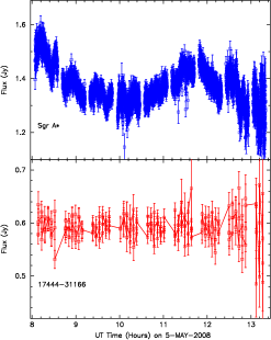
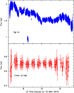
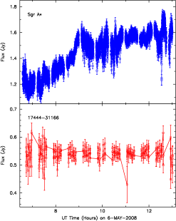
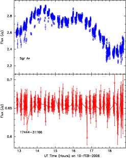
Figure 1 shows four light curves of Sgr A* on 2008 May 5, 10, 6 and 2006 February 10 using the VLA with a sampling time of 3.3sec at 7mm. The light curves of the cross calibrated calibrator are shown at the bottom of each panel in Figure 1. The flux variation is typically about 0.2–0.6 Jy with fractional change of 20-30% over 6 hours of observations. The 2008 May 10 light curve shows an unusual variation during 8.456h and 8.522h UT. This sharp drop in the flux was also simultaneously detected at 13mm with different set of VLA antennas. The drop in the flux at radio and submm wavelengths was recently discussed in the context of adiabatically cooling plasma blobs that are partially eclipsing the background quiescent emission from Sgr A* (Yusef-Zadeh et al. 2010). However, we question the reality of this dramatic drop in the flux of Sgr A* by Jy. A more detailed account of these measurements will be given elsewhere. Excluding the sharp drop in the flux of Sgr A*, a high variation with a fractional change of 40% is noted on 2010, May 10. The contamination of extended structures in the light curve can be significant for baselines less than 100k so we removed shorter baselines in constructing of all the light curves presented in Figure 1a-c (Yusef-Zadeh et al. 2009). To further minimize any contribution of extended emission, we have selected data taken with the VLA in its A configuration. Figure 1d shows the light curve constructed from the A configuration observation on 2006 February 10. The light curves corresponding to 2008 May 10 (excluding the sharp absorption feature) and 2006 February 10 show flux variations of and 0.5 Jy with mean flux of 1.6 and 2.6 Jy, respectively.
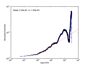
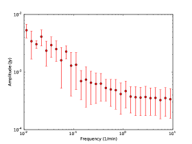
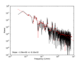
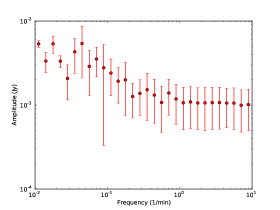
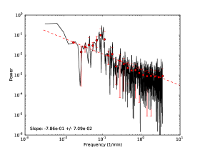
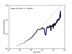
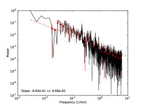
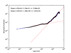
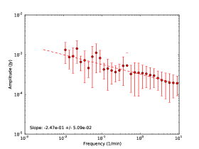
Figures 2a presents a plot of the structure function of Sgr A* on 2008 May 5 at 7mm. To examine the frequency dependence of the variability, the binned CLEAN power spectral density (PSD) and the power spectrum calculated by Uttley et al. (2002) are presented in Figure 2b,c, respectively. To check the CLEAN power spectrum analysis, the power spectrum calculation using Uttley’s technique show that the binned data points in Figure 2b,c are consistent with each other but with different normalizations. These power spectra confirm that most of the power is at low frequencies. Power-law fits to the structure function over a range between 1 and 10 minutes as well as to the PSD in Figure 2c over the entire frequencies are displayed in Figure 2a,c. On short time scales 1min the structure function and the PSDs at frequencies between 1 and 10 min-1 are constant within the error bars. However, the variability at values 2min shows a steeper slope consistent with evidence for short time scale variability. For comparison, we constructed the structure function of the calibrator 17443-31166 and found the slope of the structure function remains flat over all time scales. The flat slopes in Figure 2a,b,c at 1min are consistent with measurement errors in amplitude or white noise (Hughes, Aller & Aller 1992). For flux variability that is simply due to measurement errors with standard error , it is expected that structure function amplitude is 2.
To examine the reality of the short time variability at 1min, we have also constructed autocorrelation functions of the light curves taken on 2008, May 5. Figure 2d shows a plot of the autocorrelation function of the measurements showing a peak at zero time lag, followed by a sharp drop implying a lack of correlation on short time scales. The steep drop in the autocorrelation function is consistent with short time scale variability inferred from SF and PSDs.
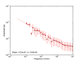
To check the validity of the analysis of the data taken on 2008 May 5, we carried out simultaneous VLBA and VLA measurements at 7mm. Due to the large interstellar scatter broadening of Sgr A*, only few short baselines of VLBA antennas could be used to investigate the nature of the variability of Sgr A* at 7 mm. The same plasma is responsible for daily time variability at centimeter wavelengths (Macquart and Bower 2006). Scintillation models predict variability at a level of 10% at 7mm wavelengths on a time scale of few days (Macquart and Bower 2006). Thus, the variability measurements presented here show large flux variability on much shorter time scales, thus, should not be affected by interstellar scintillation. Figure 3a-d show the SF, two different PSDs and the autocorrelation function of VLBA data at 7mm, all of which are consistent with short time scale variability, as measured by the VLA and shown in Figure 2. The measurements error bars in Figure 3 are high and the flat slope fitting the short time scale variation is consistent with high measurements errors. The consistent results from VLA and VLBA measurements on short time scales support the suggestion by earlier studies that the radio variability of Sgr A* arises from the inner AU of Sgr A* (Yusef-Zadeh et al. 2009) and that both show similar time scale for minute time variability.
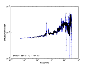
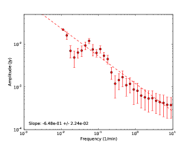
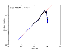
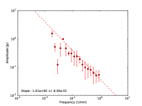
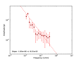
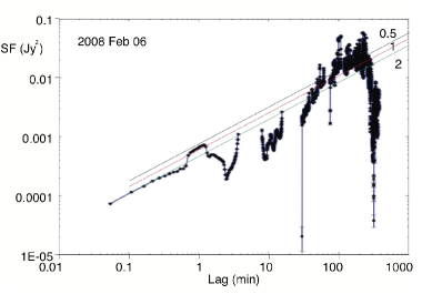
Figures 4a-d show the SF, PSDs and the autocorrelation function of VLA data taken on 2008 May 10 at 7mm. The structure function rises at short time scales, plateaus between 5 and 100 min, before rising again at longer time lags. The rapid steepening of the structure function above 300 min reflects the decline of the light curve over the duration of the observations, and the sharp drop apparent at on the very longest time scales is an artifact of the very limited sampling available at the longest lag times. It is clear that the slope of the structure function changes between minute and hourly time scales. Similar behavior has been observed in the structure function plots of X-ray data taken toward AGNs (Kataoka et al. 2001). The slopes to the CLEAN PSD and Uttley’s PSD, as shown in Figure 4b,c, range between and –0.86 and are consistent within 3 errors of each other. Power law fits to the SF at short time scales between 0.1 and 1 min and to the PSDs over their entire frequency spectra as well as the sharp drop in the autocorrelation function at 0 time lag support evidence of short time scale variability.
The structure function for the 2008 May 10 light curves, as shown in Figure 4a, differs in two ways from that for 2008 May 5. First, a number of dips in the structure function show what at face value might be considered as QPO activity. A dip is produced when a pair of measurements separated by a time lag have similar flux density. The strongest dip is seen around 20 minutes followed by weaker dips at 50 and 100 minutes. Similar dips are also noted in the structure function plot at 13mm which were taken simultaneously with 7 mm. These dips which are not detected in other three days of observations in May 2008 are caused mainly by the sharp drop in the flux of Sgr A*, as shown in Figure 1c. If we remove the sudden drop of flux, the dips in the SF disappear. Thus, we can not confirm the reality of these dips.
The second feature apparent in Figure 4a is the steepening of the slope of the structure function at 3 min down to time scales as short as 0.1 min, indicating that there is intrinsic variability on very short time scales. The reality of this short time scale variability is strengthened by the flat structure function of the calibrator. In addition, we note that the expected value of the structure function once it becomes dominated by measurement error is Jy2. The amplitude of the structure function with lag time greater than 0.1 min is higher than this, supporting the reality of such short time scale variability. These measurements suggest continuous variability from sub-minute time scale to hour time scale variability, but with varying slopes. Figure 4d shows a dramatic drop in the amplitude of the autocorrelation during the initial ten minutes which is consistent with the PSD not flatteining at higher frequencies. The steep drop in the autocorrelation function supports the intrinsic minute time scale variability.
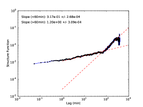
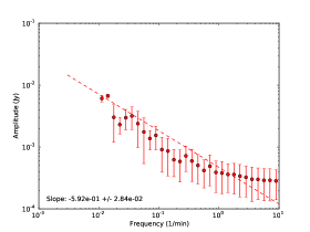
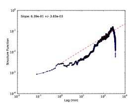
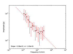
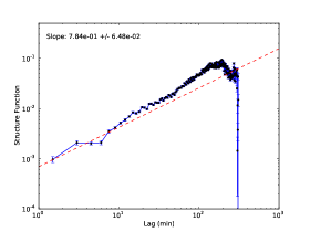
Figures 5a-c and 6a-c show the SF, CLEAN PSD and the autocorrelation function of VLA data taken on 2008 May 6 at 7 and 13mm, respectively. Figures 5a and 6a show the plots of the structure function for the 2008 May 6 light curves at 7 and 13mm, respectively. Overall, the structure function is a shallow power-law at short time scales before steepening at long time scales. Although the measurement errors of the 13mm data are greater than at 7mm, the structure function at 13mm has a similar trend to that seen at 7mm. The power-law indices at 7 and 13mm at short time scales are 0.22 and 0.32 and and at long time scales are 1.39 and 1.20, respectively. The transitions from a shallow to a steep slope of the structure function are at and 60 minutes at 7 and 13mm, respectively. The constructed CLEAN PSD and the autocorrelation of the 2008 May 6 data at 7 and 13mm show the slopes of the power spectra are not flat and that there is a steep drop in the amplitude of the autocorrelation function. These figures all show the evidence for short minute time scale variability at radio wavelengths.
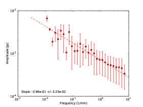
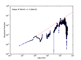
Figures 7a-c and 8a-c show the SF, CLEAN PSD and the autocorrelation function of VLA data taken on 2006 February 10 at 7 and 13mm, respectively. As pointed out earlier, these measurements should have no contamination from the extended emission from the ionized gas surrounding Sgr A*. These figures show collectively the same pattern of continuous variability from 0.1 to 250 min. The sub-minute time scale variability and the deviation from a flat slope at short time scales in the SF and high frequencies are consistent with the short time scale variability of Sgr A*. The smoothly varying slope in these high resolution observations is consistent with other low resolution measurements taken in the C configuration of the VLA. Furthermore, the steep falloff of the correlation at short time scales implies rapid and continuous fluctuations over a wide range of time scales in the flux of Sgr A*.
4 IR and X-ray Variability
Structure functions have also been calculated for several nights of Keck observations of Sgr A* (Do et al. 2009). We have used data taken with VLT, XMM-Newton and VLA observations on 2007, April 4 at IR, X-ray and radio wavelengths (Porquet et al. 2008; Dodds-Eden et al. 2009; Yusef-Zadeh et al. 2009). Figure 9a-f show the structure function and the corresponding CLEAN PSD plots of IR, X-ray, radio observations, respectively, sensitive to time lags ranging from about 0.5 to a few hundred minutes. The X-ray and IR data on 2007 April 4 revealed simultaneous bright X-ray and IR flares at the beginning of observations.
The power-law fit to the IR data implies slope of 0.9 in the structure function. Different nights of Keck observations (Do et al. 2009) show value of varying between 0.26 and 1.37 with lag times ranging between 1 to 40 minutes. The value of from VLT measurements are consistent with Keck measurements. We also note evidence of variability at about minute time scale at IR wavelengths (see also the analysis by Do et al. (2009) and Dodds-Eden et al. (2009). The slope of the CLEAN PSD at high frequencies is consistent with the short time scale variability inferred from SF analysis. There is no evidence for QPOs in the time domain that was searched. The reality of QPO activity of a hot spot orbiting Sgr A* is hotly debated mainly because of the low signal-to-noise and possible intermittent nature of such behavior (Eckart et al. 2006; Meyer et al. 2008; Do et al. 2009).
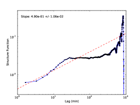
Unlike the IR structure function which is fit by a single power law, X-ray structure function and CLEAN PSD give different characterization of the variability of Sgr A* in X-rays. We note a rise at short time scales, similar to that of IR, though somewhat shallower, followed by a plateau with time lags ranging between 30 and 300 minutes before a steepening of the structure function again at longer time scales. Due to limited sensitivity and 100-second sampling of X-ray data, the flat part of the SF with time lags of few minutes indicate that there is no minute time scale variability and that the emission is dominated by white noise. The plateau time lags range between 30 and 300 minutes and is also consistent with white noise where there is no correlation of signals. At time lags greater than 300 minutes, the correlation begins again. The steepening of the structure function at 300 min is due to the large count rate difference between the beginning of the light curve when there was a bright X-ray flare and the end of the observation when the emission was at its quiescent level. The X-ray shape of the structure function plot of Sgr A* is remarkably similar to that of Mrk 421 with time lags that are an order of magnitude larger (see Figure 4c of Kataoka e al. 2001). Similarly, the mass of the black hole in Mrk 421 is estimated to be 50 times higher than the mass of Sgr A* (Barth, Ho and Sargent 2003). The characteristic time scale of X-rays from Mrk 421 is considered to place a constraint on the size of the variable X-ray emission from the base of the jet (Kataoka et al. 2001).
Figures 9e,f represents the structure function and PSD at 7mm taken simultaneously with IR and X-ray data, as part of an observing campaign that took place on 2007, April 4 (Yusef-Zadeh et al. 2009). We note a rise of the amplitude of the SF, similar to that seen in the IR structure function plot. The power-law fit to the radio data shows slope of 0.78 in the structure function which is close to that of IR data, as seen in Figure 9a. A correlation between the optically thin IR, X-ray flare and optically thick 7mm radio flare has been suggested for the strong flare that occurred on this day (Yusef-Zadeh et al. 2009; Dodds-Eden et al. 2009). The radio flare emission at 7mm was argued to be delayed with respect to the near-IR and X-ray flare emission, consistent with the plasmon picture. The similar behavior of the structure function of IR and radio data is not inconsistent with a picture that flaring activity in radio and IR wavelengths is correlated.
5 Discussion
5.1 Long Time Scale Variability
Our multi-wavelength monitoring of Sgr A* characterizes the intrinsic time variability of Sgr A* by studying the structure function of the observed light curves. Structure function analysis of the IR, X-ray and radio data suggests that most of the power falls in the long time scale fluctuation of the emission from Sgr A* and that the variation is generally aperiodic with no obvious QPO activity, confirming earlier analysis of IR data (Do et al. 2009; Meyer et al. 2008). The structure function analysis of radio data shows a number of new features, the most interesting of which is a statistically significant time variability on subminute to hourly time scales. Unlike the IR structure function, which can be well-represented by a single power law, at radio wavelengths the structure functions are more complex and could only be fit by multiple power law components.
Using the long time scale lags, we fit a power law to the PSD and SF of radio data and find the power indices of radio variability. The long time scale variability of Sgr A* at radio wavelengths characterized in the SF plots is similar to the duration of typical flares as detected in both radio and submm wavelengths (e.g., Yusef-Zadeh et al. 2006; Marrone et al. 2006). These measurements at 7 and 13mm are consistent with the power spectrum analysis of the time variability of Sgr A* suggesting intraday variability at 3mm (Mauerhan et al. 2005). The rapid decay of the SF plots at large lag times appears to reflect a turnover in the PSD of the variability. However, this turnover is probably due to an artifact of limited sampling of radio data at large time lags (see Emmanoulopoulos et al. 2010).
The hour-long flaring in radio and sub-mm has been argued to be due to adiabatic cooling of synchrotron-emitting electrons in an expanding plasma blob (Yusef-Zadeh et al. 2009). These measurements support this picture and show that the light curves peak at successively lower frequencies (submm, millimeter and then radio) as a self-absorbed synchrotron source region expands after the initial event that energizes the electrons. The emission at a particular frequency peaks as the blob becomes optically thin at that frequency, so the blob size determines the peak flux of the flare and the expansion speed determines the flare duration. The estimated expansion speed of the plasma is a few percent of , the plasma itself may be bound to Sgr A* or be embedded in the base of a jet (Maitra et al. 2009; Yusef-Zadeh et al. 2009). In this scenario, the contributions of the flares to the structure functions at 7 and 13 mm should be related to one another. To examine this, first consider the frequency-dependence of the properties of individual flares. For an electron energy spectrum the light curve of each flare follows the characteristic frequency-dependence of the plasmon model (van der Laan 1966; Yusef-Zadeh et al. 2006):
| (1) |
where the optical depth of the blob
| (2) |
and the reference optical depth is chosen so that the peak flux at frequency is and this occurs when the blob radius is . This means that is determined by , it turns out that and is a weak function of (Yusef-Zadeh et al. 2006). At frequency the peak flux
| (3) |
occurs when the blob radius is
| (4) |
Then we may rewrite the flux and optical depth at as
| (5) |
and
| (6) |
respectively. These expressions show that the flux as a function of blob radius at can be found from the light curve at through a simple linear stretch of the -axis by a factor of and a compression of the flux axis by a factor . Under the assumption that the blob has constant expansion speed, the mapping between and time is linear and the light curves behave in the same way. To summarize, the adiabatic expansion scenario implies that the amplitude and time scales of a single flare scale as and respectively, where
| (7) |
and
| (8) |
Suppose now that the variations in the light curves of Sgr A* at 7 mm arise through a superposition of flares, each with the same electron energy spectrum but with a distribution of amplitudes and time scales. Because the amplitude and time scales of the contribution of each flare scale with frequency as and respectively, the structure functions of the light curve at and are related by
| (9) |
where and are given by equations 7 and 8. In particular, note that if the structure function at is a power-law, the structure function at will also be a power law with the same index but different normalization.
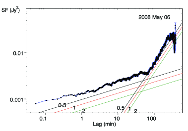
To test this hypothesis, we take the power-law fits to the structure functions at 7 mm for 2008 May 6 and 2006 February 10 and compute the 13 mm structure function predicted by eq (9), setting and to 43 and 22 GHz respectively. The amplitude of the predicted 13mm SF using our model and extrapolated from the 2008 May 06 data at 7mm is lower by 30% than that observed at 13mm. The only adjustable parameter available is , the power law index of the electron energy spectrum. We overplot the result on the measured 13 mm structure functions in Figure 10. we conclude that structure functions at 13 mm for 2008 May 6 and 2006 February 10 are quantitatively reproduced from their 7 mm counterparts for . This is consistent with earlier fits to individual large flares in other radio and sub-mm data sets (Yusef-Zadeh et al. 2006, 2009).
5.2 Short Time Scale Variability
The most interesting feature of the analysis presented here is that the structure function at radio wavelengths shows short time scale variability of Sgr A* 0.3 min with a shallower slope than seen at longer time lags. This is the shortest time scale variability that has been detected toward Sgr A* and suggests that radio emission may arise from the innermost region of the accretion flow. The best case for minute time scale variability is seen in Figure 3a and 5 where the structure function rises for lag times greater than 0.3 minutes. In both cases, the amplitude of the structure function at time scales greater than 0.3 min for data taken on 2008 May 10 and 2006 February 10 is greater than twice the mean square of the measurement errors, providing the evidence for subminute time scale variability. The transition time scales where the slope of the SF changes was estimated from 30 and 60 minutes at 7 and 13mm. These transitions suggest that the physical mechanism for production of the variability may be different. The different lag time at 7 and 13mm can be accounted for in terms of optical depth effect of hourly time scale variability in an adiabatic expanding synchrotron source. Previous time delay determinations based on individual identified flare events show a time delay of 20-40 minutes between the peaks of emission at 7 and 13mm (e.g., Yusef-Zadeh et al. 2009) as well as the increase of the duration of the flare emission in the time domain at lower frequencies. The latter effect is likely to be responsible for the transition in the slope seen in the structure function analysis.
As noted before, the component of the variability shows a different slope at short time scale than that at hourly time scale which dominates the power spectrum of the variable emission. The steepening of the slope at longer time lags reflects the systematic increase of the flux from Sgr A* over the course of the observations, and is removed if a linear increase in flux is subtracted from the light curve. After subtracting off the secular change over several hours of observations, the structure function shows that there is continuous variability at 7mm on minute to hourly time scale and that there is variability on a longer time scale than several hours. Given that hourly time scale variability is interpreted in the context of adiabatically expanding hot plasma blob with sub-relativistic expansion, it is natural to consider that the short time scale variability is also optically thick.
Sub-minute time scale variability places a strong constraint on the size of the emission region. Light crossing time arguments place an upper limit comparable to the Schwarzschild radius of Sgr A*, i.e. AU for a Galactic center distance of 8 kpc (Doeleman et al. 2008). The flux variation on minute time scales at 7 mm is 10-30 mJy. Assuming that this is produced by adiabatic expansion of a uniform synchrotron source with an electron spectrum, the optical depth at the peak . Assuming that the electron spectrum extends between 1 and 100 MeV and that there is equipartition between the magnetic field and the electrons, then a peak flux of 30 mJy is obtained for cm and magnetic field strength G. The flare time scale is 60 seconds for an expansion speed . For a peak flux of 10 mJy we obtain cm, G and respectively. Clearly this model would have difficulty producing 30 mJy flux variations on 0.3 min time scales, but 10 mJy fluctuations would be viable.
Associating a proton with each synchrotron-emitting electron, the mass of the source region for the 30 mJy case is g. Continual variations on a 60 second time scale then imply a processing rate of material yr-1. The energy in magnetic fields and relativistic electrons in the expanding source region declines on the expansion timescale, implying a transfer of energy into the immediate surroundings at a rate . These rates will be somewhat higher if their are multiple overlapping flares at any given time.
The origin of these short time fluctuations is unclear, but the inferred explosive expansion of the emitting plasma at near-light speeds is suggestive of that they might feed into an outflow or jet. We note that the inferred scale length corresponding to one-minute light travel time is comparable to the time averaged spatially resolved 0.1AU scale observed at 1.3mm by (Doeleman et al. 2008). The quiescent variable emission from Sgr A* could then be interpreted mainly as an ensemble average of numerous flares that are detected on minute-time scale. This short time scale emission or quiescent variability could be due to fluctuations in the accretion flow of Sgr A* due to magnetic field fluctuations resulting from MRI, as recent MHD simulations in a number of studies indicate.
6 Conclusions
In conclusion, the rapid fluctuation of emission from Sgr A* allows us to probe the spectacular activities of the central engine at remarkably small spatial scales. We have constructed structure functions, power spectra and autocorrelation functions using radio, IR and X-ray data in order to characterize the time variability of Sgr A*. These plots indicate that most of the power in the time variability is on hourly time scales. However, the shapes of the structure function in X-rays and radio wavelengths are different than that of IR data. Radio continuum variability is detected to be continuous from short subminute time scale to long hourly time scale. We argue that rapid fluctuations of the radio emission imply rapid expansion that could feed the base of an outflow or jet in Sgr A*. The bulk of the continuum flux from Sgr A* at radio and submm wavelengths is believed to be generated in its accretion disk. The localization and characterization of the source of variable continuum emission from Sgr A* give us opportunities to further our understanding of the launching and transport of energy in the nuclei of Galaxies.
References
- Alexander (1997) Alexander, T. 1997, MNRAS 285, 891
- Arshakian et al. (2010) Arshakian, T. G., Leon-Tavares, J., Lobanov, A. P. et al. 2010, MNRAS, 401, 1231
- Barth et al. (2003) Barth, A. J., Ho, J. C., & Sargent, W. L. W. 2003, ApJ, 583, 134
- Bower et al. (2004) Bower, G. C., Falcke, H., Herrnsein, R. M., Zhao J.-H., Goss, W. M. & Backer, D. C. 2004, Science, 304, 704
- Chan et al. (2009) Chan, C.-K., Liu, S., Fryer, C. L., Psaltis, D., Ozel, F., Rockefeller, G. and Melia, F. 2009, ApJ, 701, 521
- Do et al. (2009) Do, T., Ghez, A. M., Morris, M. R., Yelda, S., Meyer, L., Lu, J. R., Hornstein, S. D. & Matthews, K. 2009, ApJ, 691, 1021
- Doeleman et al. (2008) Doeleman, S. S., Weintroub, J., Rogers, A. E. E., Plambeck, R., Freund, R., Tilanus, R. P. J. et al. 2008, Nature, 455, 70
- Dodds-Eden et al. (2009) Dodds-Eden, K. et al. 2009, ApJ, 698, 676
- Eckart et al. (2006) Eckart, A., Schodel, R., Meyer, L., Trippe, S. Ott, T. and Genzel, R. 2006, A&A, 455, 1
- Edelson and Krolik (1988) Edelson, R. A., & Krolik, J. H. 1988, ApJ, 333, 646
- Emmanoulopoulos et al. (2010) Emmanoulopoulos, D., McHardy, I. M., and Uttley, P. 2010, MNRAS, 404, 931
- Ghez et al. (2008) Ghez, A. M., Salim, S., Weinberg, N. N., Lu, J. R., Do, T., Dunn, J. K., Matthews, K., Morris, M. R., Yelda, S., Becklin, E. E. and Kremenek, T. et al. 2008, ApJ, 689, 1044
- Gillessen et al. (2009) Gillessen, S. et al. 2009, ApJ, 692, 1075
- Goldston et al. (2005) Goldston, J. E., Quataert, E. and Igumenshchev, I. V. 2005, ApJ, 621, 785
- Hawley et al. (2002) Hawley, J. F. & Balbus, S. A. 2002, ApJ, 573, 738
- Hughes et al. (1992) Hughes, P.A., Aller & Aller, 1992, ApJ, 396, 469
- Kataoka et al. (2001) Kataoka, J., Takahashi, T., Wagner, S. J. et al. 2001, ApJ, 560, 659
- Liu et al. (2004) Liu, S., Petrosian, V., & Melia, F. 2004, ApJ, 611, L101
- Macquart and Bower (2006) Macquart, J. P. & Bower, G.C. 2006, ApJ, 641, 302
- Marrone et al. (2006) Marrone, D. P., Moran, J. M., Zhao, J.-H. & Rao, R. 2006, Journal of Physics: Conference Series, Volume 54, Proceedings of ”The Universe Under the Microscope - Astrophysics at High Angular Resolution”, held 21-25 April 2008, in Bad Honnef, Germany. Editors: Rainer Schoedel, Andreas Eckart, Susanne Pfalzner and Eduardo Ros, pp. 354-362
- Melia & Falcke (2001) Melia, F. & Falcke, H. 2001, ARA&A, 39, 309
- Maitra et al. (2009) Maitra, D., Markoff, S. & Falcke, H. 2009, A&A, 508, L13
- Mauerhan et al. (2005) Mauerhan, J. C., Morris, M., Walter, F. & Baganoff, F. K. 2005, ApJ, 623, L25
- McHardy et al. (2006) McHardy, I. M., Koerding, E., Knigge, C., Uttley, P. et al. 2006, ApJ, 444, 730
- Meyer et al. (2008) Meyer, L., Do, T., Ghez, A., Morris, M. R., et al. 2008, ApJ, 688, L17
- Meyer et al. (2009) Meyer, L., Do, T., Ghez, A., Morris, M. R., et al. 2009, ApJ, 694, L87
- Moscibrodzka et al. (2009) Moscibrodzka, M., Gammie, C. F., Dolence, J. C. 2009, ApJ, 706, 497
- Porquet et al. (2008) Porquet, D., Grosso, N., Predehl, P., Hasinger, G., Yusef-Zadeh, F., Aschenbach, B., et al. 2008, A&A, 488, 549
- Reid & Brunthaler (2004) Reid, M. J. & Brunthaler, A. 2004, ApJ, 616, 872
- Roberts et al. (1987) Roberts, D. H., Lehar, J., and Dreher, J. W. 1987, ApJ, 93, 968
- Simonetti et al. (1985) Simonetti, J. H., Cordes, J. M. and Heeschen, D. S. 1985, ApJ, 296, 46
- Uttley et al. (2002) Uttley, P., McHardy, I. M., and Papadakis, I. E. 2002, MNRAS, 332, 231
- van der Laan (1966) van der Laan, H. 1966, Nature, 211, 1131
- Yuan et al. (2003) Yuan, F., Quataert, E., & Narayan, R. 2003, ApJ, 598, 301
- Yusef-Zadeh et al. (2006) Yusef-Zadeh, F., Roberts, D., Wardle, M., Heinke, C. O. and Bower, G. C. 2006, ApJ, 650, 189
- Yusef-Zadeh et al. (2009) Yusef-Zadeh, F., Bushouse, H., Wardle, M., Heinke, C. et al. 2009, ApJ, 706, 348