High Resolution Spectroscopy during Eclipse
of the Young Substellar Eclipsing Binary 2MASS 0535$-$0546.
I. Primary Spectrum: Cool Spots versus Opacity Uncertainties

Abstract

We present high-resolution Keck optical spectra of the very young substellar eclipsing binary 2MASS J05352184$-$0546085, obtained during eclipse of the lower-mass (secondary) brown dwarf. The observations yield the spectrum of the higher-mass (primary) brown dwarf alone, with negligible ($\sim$1.6%) contamination by the secondary. We perform a simultaneous fine-analysis of the TiO-$\epsilon$ band and the red lobe of the K I doublet, using state-of-the-art PHOENIX dusty and cond synthetic spectra. Comparing the effective temperature and surface gravity derived from these fits to the empirically determined surface gravity of the primary ($\log g$ = 3.5) then allows us to test the model spectra as well as probe the prevailing photospheric conditions. We find that: (1) fits to TiO-$\epsilon$ alone imply $T_{\rm eff}$ = 2500$\pm$50K; (2) at this $T_{\rm eff}$, fits to K I imply $\log g$ = 3.0, 0.5 dex lower than the true value; and (3) at the true $\log g$, K I fits yield $T_{\rm eff}$ = 2650$\pm$50K, $\sim$150K higher than from TiO-$\epsilon$ alone. On the one hand, these are the trends expected in the presence of cool spots covering a large fraction of the primary’s surface (as theorized previously to explain the observed $T_{\rm eff}$ reversal between the primary and secondary). Specifically, our results can be reproduced by an unspotted stellar photosphere with $T_{\rm eff}$ = 2700K and (empirical) $\log g$ = 3.5, coupled with axisymmetric cool spots that are 15% cooler (2300K), have an effective $\log g$ = 3.0 (0.5 dex lower than photospheric), and cover 70% of the surface. On the other hand, the trends in our analysis can also be reproduced by model opacity errors: there are lacks in the synthetic TiO-$\epsilon$ opacities, at least for higher-gravity field dwarfs. Stringently discriminating between the two possibilities requires combining the present results with an equivalent analysis of the secondary (predicted to be relatively unspotted compared to the primary).

1 Introduction

2MASS J05352184$-$0546085 (henceforth 2M0535), a very young system located in the Orion Nebula Cluster (ONC), has recently been identified by Stassun et al. (2006, hereafter SMV06) as the first known substellar eclipsing binary (EB). EBs allow exquisitely precise direct determinations of the component masses and radii, and thus the surface gravities ($\log g$), as well as the ratio of their luminosities (or equivalently, ratio of their effective temperatures, $T_{\rm eff}$). As such, 2M0535 permits the first stringent tests of both the theoretical evolutionary models and the synthetic spectra that are widely employed to characterize the vast majority of brown dwarfs (for which direct measurements of mass, radius, and surface gravity are not possible).

The parameters of the system found by SMV06 were refined with more data by Stassun et al. (2007, hereafter SMV07) and still further by Gómez Maqueo Chew et al. (2009, hereafter G09). SMV07 found a spectral type of M6.5$\pm$0.5 for the primary (higher-mass) component, suggesting $T_{\rm eff}$ $\approx$ 2700K (Golimowski et al., 2004). The latest analysis by G09 confirms the initial findings that: (1) Both components of 2M0535 are moderate mass brown dwarfs ($M_{1}$ = 0.0572$\pm$0.0033 M_⊙, $M_{2}$ = 0.0366$\pm$0.0022 M_⊙); (2) their radii ($R_{1}$ = 0.690$\pm$0.011 R_⊙, $R_{2}$ = 0.540$\pm$0.009 R_⊙) are consistent with the theoretical prediction that young brown dwarfs of a given mass should be much larger than their field counterparts; and (3) the $T_{\rm eff}$ ratio of the components ($T_{\rm eff}$_,2/$T_{\rm eff}$_,1 = 1.050$\pm$0.004) shows an unexpected reversal, with the primary being cooler than the lower-mass secondary.

The reversal in temperatures is not predicted by any set of theoretical evolutionary tracks. To explain it, Chabrier et al. (2007, hereafter CGB07) proposed that strong magnetic fields on the primary suppress its interior convection and also produce cool surface spots; neither effect is included in the standard evolutionary models, and both would act to depress its $T_{\rm eff}$. Reiners et al. (2007, hereafter R07) subsequently found that, compared to the secondary, the primary is a relatively fast rotator with strong chromospheric ${{\rm H}\alpha}$ emission, which supports the presence of strong magnetic fields in the latter. G09 then showed that the observed small-amplitude residual (non-eclipse) variations in the 2M0535 lightcurve, modulated at the rotational periods of the primary and secondary, can be well reproduced by cool spots asymmetrically covering a small fraction ($\lesssim$ 10%) of both components’ surfaces. While such small spots cannot explain the temperature reversal, G09’s analysis does indicate that spots are at least present. Moreover, they cannot rule out the very large ($\sim$ 50% areal coverage) spots on the primary required to explain the temperature reversal, as long as these are arranged symmetrically about the rotation axis (e.g., polar spots, equatorial bands, or ‘leopard spots’).

Additionally, through analysis of the optical to mid-IR spectral energy distribution (SED), Mohanty et al. (2009, hereafter MSM09) showed that: ongoing accretion is highly unlikely in the 2M0535 system, lending credence to the R07 conclusion that the ${{\rm H}\alpha}$ emission in the primary is chromospheric; and the system SED is consistent with effective temperatures of [$T_{\rm eff}$_,1, $T_{\rm eff}$_,2] $\sim$ [2700, 2900]K, in agreement with the mid-M spectral types of the components rather than with the much lower $\sim$ [2300, 2450]K proposed by CGB07 within their theory of $T_{\rm eff}$ reversal via magnetic field effects. Combining their results with the others cited here, MSM09 concluded that while magnetically-induced spot/convection effects probably do play an important role in determining the $T_{\rm eff}$ of the 2M0535 primary, as advocated by CGB07 (and as indeed seems to be the case for active field dwarfs; Morales et al., 2008), the theory is as yet insufficiently developed quantitatively, and small age variations between the components may play a significant role as well (as in fact appears to be the case in another young EB, albeit with stellar-mass components, Par 1802; Stassun et al., 2008).

Finally, subsequent to MSM09’s work, MacDonald & Mullan (2009) have proposed a theory wherein magnetic fields inhibit the onset of convection (though do not suppress it entirely) throughout the 2M0535 primary, instead of just in the upper-most super-adiabatic layers as in the theory of CGB07. The theory appears to reproduce the observations of 2M0535AB without invoking non-coevality or very large surface spots on the primary; this competing scenario must be evaluated as well.

In this paper, we present Keck HIRES observations of 2M0535 obtained during eclipse so as to isolate the spectrum of the higher-mass, lower-$T_{\rm eff}$ primary brown dwarf. Comparing the observed spectrum with state-of-the-art brown-dwarf atmosphere models, we test the ability of these models to correctly reproduce the accurately known surface gravity ($\log g$ = 3.52$\pm$0.03; G09, ), and in the process we directly probe the prevailing photospheric conditions of the primary brown dwarf in the 2M0535 system.

2 Observations and Data Reduction

We observed 2M0535 on the night of UT 2007 Oct 23 with the High Resolution Echelle Spectrometer (HIRES) on Keck-I. We observed in the spectrograph’s “red” (HIRESr) configuration with an echelle angle of $-0.403$ deg and a cross-disperser angle of 1.703 deg. In this configuration, the two features of primary interest in this paper, TiO $\lambda\lambda$8435–8455 and K I $\lambda$7700, fall on the “green” chip, in echelle orders 42 and 46, respectively. We used the OG530 order-blocking filter and the 1$\farcs$15$\times$7$\farcs$0 slit, and binned the chip during readout by 2 pixels in the dispersion direction. The resulting resolving power is $R\approx 34\,000$, with a 3.7-pixel ($\sim 8.8$ km s^-1) FWHM resolution element.

We obtained three consecutive integrations of 2M0535, each of 2400 s. ThAr arc lamp calibration exposures were obtained before and after the 2M0535 exposures, and sequences of bias and dome flat-field exposures were obtained at the end of the night. The 2M0535 exposures were processed along with these calibrations using standard IRAF tasks and the MAKEE reduction package written for HIRES by T. Barlow. The latter includes optimal extraction of the orders as well as subtraction of the adjacent sky background. The three exposures of 2M0535 were processed separately and then median combined with cosmic-ray rejection into a single final spectrum. The signal-to-noise (S/N) of the final spectrum is $\sim 15$ per resolution element.

Importantly, we intentionally chose the observations to coincide exactly with the secondary eclipse, i.e. when the lower-mass, smaller, higher-$T_{\rm eff}$ secondary component was behind the primary as seen from Earth. The first exposure started at UT 12:20 h, and the third exposure ended at UT 14:22 h, corresponding to orbital phases of 0.0709 and 0.0794, respectively, during which time the secondary is almost completely blocked (cf. Fig. 3 in SMV07, ). Integrated over the entire 2-hr observation, the total light contribution from the secondary was $\approx$1.6%. The light contribution from the secondary was calculated using the accurately determined radius ratio, temperature ratio, and orbital parameters, including the orbital inclination, from the light curve modeling performed in G09. Thus the resulting spectrum is effectively that of the primary alone.

3 Synthetic Spectra

We use the latest version of synthetic spectra for plane-parallel atmospheres generated using the PHOENIX code, designated AMES-Cond (version 2.4) and AMES-Dusty (version 2.4) (Allard et al., 2001). These synthetic spectra have become broadly used in the literature on low-mass stars and brown dwarfs especially at young ages. In addition, these model spectra are incorporated into the commonly used stellar evolution models of Baraffe et al. (1998) as well as in the CGB07 models discussed in Sec. 1. Thus one of our aims in selecting the PHOENIX synthetic spectra here is to assess these commonly used models in the context of brown dwarf evolution.

The PHOENIX code (Hauschildt & Baron, 1999) is a general purpose stellar atmosphere model tool that makes use of very complex atomic models and line blanketing by hundreds of millions of atomic and molecular lines. The PHOENIX models used here incorporate the most recent AMES line lists for both TiO (Langhoff, 1997; Schwenke, 1998) and H₂O (Partridge & Schwenke, 1997). A good treatment of H₂O is essential for analyzing optical spectra, even though H₂O opacity dominates only in the infrared (TiO opacity is more important in the optical). This is because the overall H₂O opacity is larger, and its lines occur closer to the peak of the SED than those of TiO, at the low $T_{\rm eff}$ in M spectral types. Consequently, changes in the H₂O opacity have a substantial effect on the atmospheric temperature structure and thus on the emergent spectrum even in the optical. A total of about 500 million molecular lines are currently included in the models; of these, $\sim$207 million are lines of H₂O, and $\sim$172 million are of TiO (Allard et al., 2000, 2001). Here we use solar-metallicity models ([M/H]=0.0). While the metallicity of 2M0535 is not explicitly known, a large deviation from solar is not expected for a young object in a nearby star-forming region. We discuss potential metallicity effects on our results in more detail in §6.2.

Dust formation is another potentially important effect in the low-temperature atmospheres of M-type objects; grains affect the atmospheric structure as well as the emergent flux. Both models we examine treat grain formation self-consistently, through chemical equilibrium calculations (see Allard et al., 2001). Under physical conditions where the chemical equations imply no grain formation, the cond and dusty spectra are identical; in the models, this occurs for $T_{\rm eff}$ $\gtrsim$ 2500K. For the latter temperatures, therefore, either set of synthetic spectra may be used. The difference between the two is in their treatment of dust settling, once grains have formed. The two models represent the two limits of settling: dusty models treat the case where grains form and remain suspended in the photosphere, while the cond ones are applicable when dust has formed but subsequently settled (“condensed”) out of the photosphere entirely. Observations of field dwarfs indicate that dust settling becomes important only in the L types (e.g., Schweitzer, 2001). For the mid-M spectral type of 2M0535, dust formation may occur but the grains are likely to remain in the photosphere (Jones & Tsuji, 1997, M04). We thus use dusty models for $T_{\rm eff}$ $<$ 2500K, and cond models for $T_{\rm eff}$ $\geq$ 2500K (where no dust forms).

4 Methodology

We wish to determine the $T_{\rm eff}$ and surface gravity ($\log g$) of the higher-mass component of 2M0535 (the “primary,” hereafter 2M0535A) from comparisons to synthetic spectra. As Mohanty et al. (2004, hereafter M04) have shown, two ideal regions for this analysis are the TiO-$\epsilon$ bandheads at $\lambda\lambda\lambda$8435,8445,8455, and the red-lobe of the K I doublet at $\lambda$7700 (the blue lobe falls in the gap between echelle orders in the HIRES setting used). In particular, the TiO bandheads are very sensitive to $T_{\rm eff}$, but negligibly so to gravity, while the K I absorption is sensitive to both; using the two regions in tandem therefore enables one to disentangle and individually determine these two parameters.

Comparing the data to models requires some modifications to both. These are discussed in detail in M04; the salient points are as follows. The models are rotationally broadened (using Gray’s methodology (Gray 1992), with a standard limb-darkening parameter of 0.6) by 10 km s^-1 to match the observed $v\sin i$ of 2M0535A (R07), and further broadened by convolution with a Gaussian profile to match the instrumental broadening (finite resolution) of the data. Since our data are not flux-calibrated, comparison to the models also requires some form of scaling. This is accomplished by normalizing both the data and models by their average flux over a narrow region of pseudo-continuum just outside the absorption lines of interest: over $\lambda\lambda$[8402.5–8411.5] for the the TiO-$\epsilon$ region, and over $\lambda\lambda$[7707.5–7709.5] for the K I region (wavelengths in the laboratory rest-frame). Recall that the data are also flat-fielded, which removes the blaze-function but preserves the innate shape of the stellar spectrum. Our normalization procedure then ensures that the data and models are only ‘anchored’ over a narrow wavelength range, but otherwise unconstrained, so the models need to match not only the absorption bands, but also the shape and slope of the continuum, to ensure a good fit. This provides an additional check on the veracity of the preferred fits.

For comparisons to the stellar spectrum, we first use the dusty and cond models depending on the $T_{\rm eff}$  being tested, as described in §3 (cond for $\geq$ 2500K); the results are described in §5. We then model the stellar spectrum as a combination of a naked photosphere and cool spots, as discussed in §6.3. For this analysis, the photosphere and spot are represented by different spectra, depending on the adopted temperature of each (e.g., for a 2700K photosphere and a 2300K cool spot, we use cond for the former and dusty for the latter). Both spectra are individually rotationally and instrumental-Gaussian broadened, and then coadded in the ratio of the adopted spot covering fraction (for a covering fration $f$, the final spectrum is given by $f$ times the spot spectrum + $(1-f)$ times the photospheric spectrum). The addition is performed prior to the normalization described above, to preserve the ratio of the spot to photospheric flux arising from their differences in both temperature and covering fraction.

Finally, we note that the synthetic spectra were originally constructed at intervals of 100K and 0.5 dex in $T_{\rm eff}$ and $\log g$ respectively. We have linearly interpolated between adjacent spectra (before normalization) to construct a finer final grid of models, with steps of 50K in $T_{\rm eff}$ and 0.25 dex in $\log g$.

5 Results

We begin with a general presentation of the fitting results and then quantify the uncertainties in the best fits.

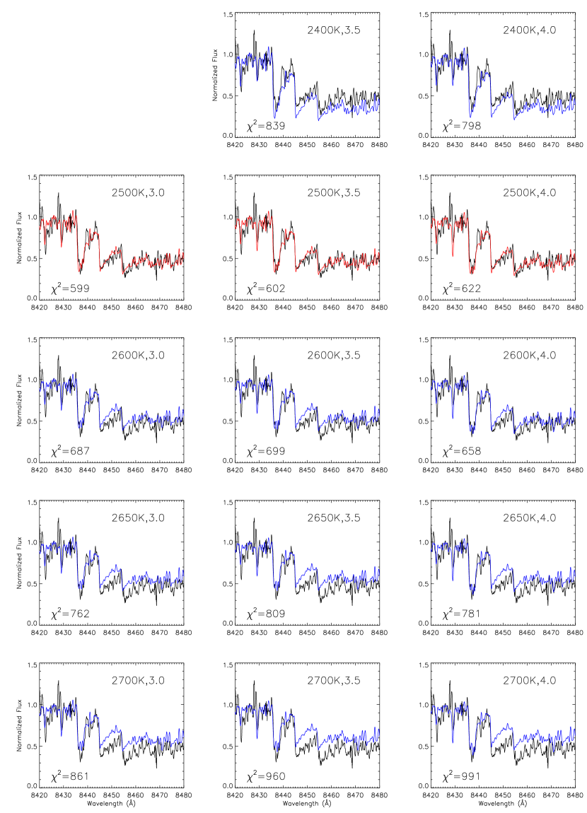
Figure 1: Observed TiO-$\epsilon$ region in 2M0535A (black) compared to Dusty ($<$ 2500K) and Cond ($\geq$ 2500K) models. Best-fit model (Cond 2500K) shown in red; all others, which clearly diverge from the data by eye, shown in blue. Note that the model fits are very insensitive to gravity over the 1 dex range plotted. See §5. This figure is shown in color in the electronic version only.

TiO-$\epsilon$: Fig. 1 shows the comparison between data and synthetic spectra in the TiO-$\epsilon$ region, which has three bandheads at $\sim$ $\lambda\lambda\lambda$8435,8445,8455. We plot models at $\log g$ = 3.0, 3.5 and 4.0 (bracketing the empirically known value of 3.5), and $T_{\rm eff}$ = 2400–2700K in steps of 100K (2650K is also shown to facilitate a comparison to K I, as we will discuss shortly). As expected, the model TiO is hardly sensitive to gravity over the 1 dex range plotted, but highly sensitive to temperature, with the bandheads at $\lambda\lambda$8445,8455 rapidly strengthening with decreasing $T_{\rm eff}$. We see that the 2500K model (in red) clearly fits the data very well, while cooler and hotter models (in blue) just as clearly do not. Given that even a 100K deviation from the best fit is evident to the eye, our precision in $T_{\rm eff}$ determination by eye is likely to be $\sim\pm$50K (in agreement with M04). From the TiO-$\epsilon$ fits, therefore, we would infer $T_{\rm eff}$ $\approx$ 2500K$\pm$50K.

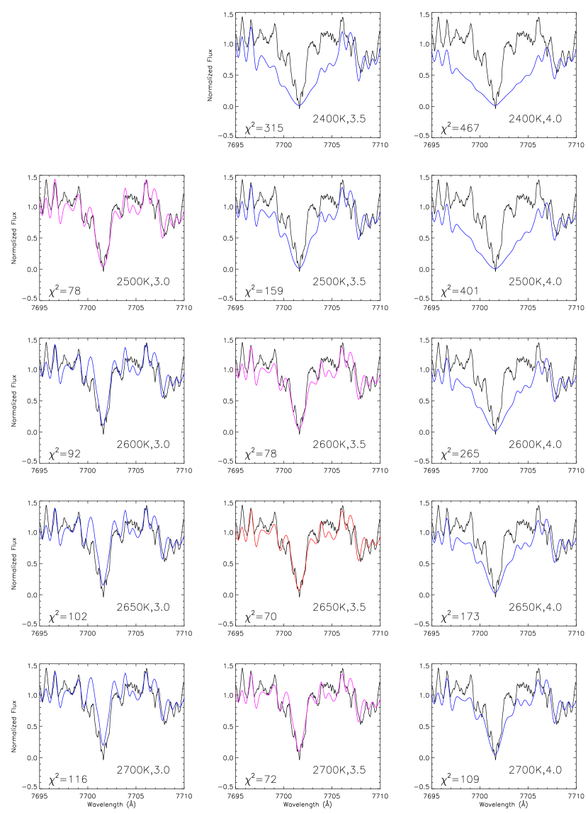
Figure 2: Observed red lobe of K I in 2M0535A (black) compared to Dusty ($<$ 2500K) and Cond ($\geq$ 2500K) models. Best-fit models (Cond [2500K, log $g$ = 3.0] and [2650K, log $g$ = 3.5]) shown in red; worse but still admissible fits by eye shown in purple; and all others, which clearly diverge from the data, shown in blue. Note that the K I absorption is sensitive to both $T_{\rm eff}$  and gravity: a 150K increase in $T_{\rm eff}$  compensates for a 0.5dex rise in log $g$. At $T_{\rm eff}$  = 2500K, corresponding to the best-fit to TiO-$\epsilon$ (Fig. 1), the K I implies log $g$ = 3.0, while at the empirically determined log $g$ = 3.5, it implies $T_{\rm eff}$  = 2650K. See §5. This figure is shown in color in the electronic version only.

K I and TiO-$\epsilon$: Fig. 2 shows the comparison between the observed and model K I $\lambda$7700, over the same range of $\log g$ and $T_{\rm eff}$ plotted in Fig. 1 for TiO-$\epsilon$. We immediately see, as pointed out by M04, that the synthetic K I is sensitive to both gravity and temperature, becoming rapidly broader and deeper with either increasing gravity or decreasing $T_{\rm eff}$. At the $T_{\rm eff}$ = 2500K inferred from TiO-$\epsilon$ above, the best fit to K I is clearly obtained at $\log g$=3.0. The model at $\log g$ = 3.5, for the same $T_{\rm eff}$, is obviously discrepant with the data; a conservative estimate of the error in this by-eye fit is $\sim$$\pm$0.25 dex (in agreement with M04, ). Thus, simultaneous model fits to TiO-$\epsilon$ and K I imply $T_{\rm eff}$ $\approx$ 2500K and $\log g$ $\approx$ 3.0. This inferred gravity is lower than the empirical value of 3.52$\pm$0.03 by $\sim$0.5 dex.

Fig. 2 also shows that, if we impose the empirical $\log g$ of 3.5, a very good fit to K I is obtained at $T_{\rm eff}$ $\approx$ 2650K. This is $\sim$150K higher than derived from the TiO-$\epsilon$ fits alone; as Fig. 1 shows, the synthetic TiO-$\epsilon$ are incompatible with this temperature. We note that 2650K is consistent with $T_{\rm eff}$ estimates for field dwarfs of the same $\sim$M6.5 spectral type as the primary (e.g., Golimowski et al., 2004; Slesnick et al., 2004), while the 2500K indicated by TiO-$\epsilon$ is somewhat low in comparison.

To better quantify the uncertainties in the fitting results of Figs. 1 and 2, we show the chi-square results for the data-model comparisons in Fig. 3. The TiO comparisons were carried out over the wavelength range [8420:8480]Å  (which includes all three bandheads; see Fig. 1), while the KI comparisons were over the range [7699:7706]Å  (corresponding to the entire line, till the pseudo-continuum is reached on either side of line-center; see Fig. 2). These ranges correspond to 69 data points for KI, and 599 for TiO.

The plot clearly shows that a degeneracy exists between $T_{\rm eff}$ and $\log g$ in the KI line, as discussed above. There are two global minima over the range of temperatures and gravities examined, one at $T_{\rm eff}$ $\approx$ 2650K and $\log g$ $\approx$ 3.5, and another at $T_{\rm eff}$ $\approx$ 2850K and $\log g$ $\approx$ 4.0. That is, a $\sim$200K decrease in temperature can compensate for a 0.5 dex decrease in gravity (as also found by M04). Thus, at the empirical $\log g$ of 2M0535, ($\log g$ = 3.5), the best-fit $T_{\rm eff}$ from KI is 2650K, in agreement with our by-eye estimate above. The corresponding 1-$\sigma$ uncertainty is 30K. The TiO lines strongly indicate $T_{\rm eff}$ = 2500$\pm$10K, again as found above. At this $T_{\rm eff}$, the K I line is marginally well fit at the 3-$\sigma$ contour level with $\log g$ = 3.0$\pm$0.05. Thus, the detailed chi-square comparisons are in excellent agreement with our fits-by-eye results for $T_{\rm eff}$ and $\log g$.

To summarize: (1) fits to TiO-$\epsilon$ yield $T_{\rm eff}$ = 2500$\pm$10K; (2) adopting this $T_{\rm eff}$, fits to K I $\lambda$7700 imply $\log g$ = 3.0$\pm$0.05, which is $\sim$0.5 dex lower than the known gravity of the primary; and (3) adopting the known value of $\log g$ = 3.5 instead, fits to K I imply $T_{\rm eff}$ = 2650$\pm$30K, which is $\sim$150K higher than, and incompatible with, the value from TiO-$\epsilon$ alone.

We note here that, while the best-fit chi-square values are the same as obtained by eye, the formal uncertainties cited above for the chi-square analysis, obtained via interpolation over the model grid, are significantly smaller than the model grid spacing (50K in $T_{\rm eff}$ and 0.25 dex in $\log g$). We therefore adopt the grid spacing of 50K and 0.25 dex as a conservative estimate of our uncertainties for the rest of the paper (corresponding to the same errors assumed for the fits by eye).

The discrepancies embodied in the above results may be due to lacks in the synthetic spectra, or an indication of real photospheric conditions. We discuss each in turn below.

6 Discussion: Possible Interpretations of the Discrepancies in $T_{\rm eff}$ and $\log g$

6.1 Model Opacity Uncertainties

Reiners (2005, hereafter R05) has compared the synthetic TiO spectra to observations of a sample of early to mid-M field dwarfs, whose $T_{\rm eff}$ and surface gravities are well-constrained via interferometric radius measurements. He shows that the model TiO-$\epsilon$ bands systematically underestimate the temperatures of these objects. Assuming that uncertainties in the $\epsilon$-band model oscillator strengths—$f_{\rm el}$($\epsilon$)—are to blame, R05 estimates that $f_{\rm el}$($\epsilon$) 70% higher than adopted in the models would remove the discrepancy in the field dwarfs. Moreover, problems with $f_{\rm el}$($\epsilon$) should produce an analogous effect in young low-gravity brown dwarfs as well. R05 predicts that a 70% underestimation of $f_{\rm el}$($\epsilon$) would yield a 150–200K underestimation of $T_{\rm eff}$ in such young dwarfs, and an attendant $\log g$ (derived by imposing this $T_{\rm eff}$ on the gravity-sensitive alkali lines, as in our analysis above) too low by $\sim$0.3 dex. These results are in qualitative and quantitative agreement with the results presented above for 2M0535.

The above prediction for young cool dwarfs is predicated on the assumption of problematic oscillator strengths. This is by no means proved, however; it may be that the fault lies in the adopted model equation of state instead (A. Reiners and P. Hauschildt, private comm., 2009), perhaps related to uncertainties in dust formation. In the latter case, it is not evident that the field dwarf discrepancies would necessarily be replicated in young objects. The steps required to resolve this issue are discussed further in §7. For now, we simply point out that the direction and magnitude of the $f_{\rm el}$($\epsilon$)-related $T_{\rm eff}$ and $\log g$ discrepancies predicted by R05 for young brown dwarfs are consistent with those found in our analysis of the 2M0535 primary. As such, lacks in the synthetic spectra remain a viable explanation for our results.

6.2 Metallicity Effects

Alternatively, we have assumed a solar metallicity for the 2M0535 system (i.e., used synthetic spectra with log[M/H] $\equiv$ log[(M/H)/(M_⊙/H_⊙)] = 0.0); can non-solar abundances resolve the $T_{\rm eff}$ and $\log g$ discrepancies we find? We do not think so, for the following reason.

Metallicity variations affect the spectra as follows. Higher metallicity reduces the number of Hydrogen particles (which are the main source of collisional broadening) relative to metals; it also implies a decrease in pressure at a given optical depth (because of higher opacity). Both effects tend to yield a narrower alkali line at higher metallicity, just as decreasing gravity does at solar metallicity (Schweitzer et al. 1996; Basri et al. 2000; Mohanty et al. 2004). This could lead to an underestimated $\log g$ from K I. Simultaneously, higher metallicity leads to an increase in the relative abundance of Titanium and Oxygen, and also causes a decrease in temperature at a given optical depth (again due to higher opacity). Both effects lead to a strengthening of the TiO bands at higher metallicity, just as decreasing $T_{\rm eff}$ does at solar metallicity (Leggett 1992; Mohanty et al. 2004). In summary, a higher metallicity mimics lower gravity and lower $T_{\rm eff}$. Thus, if we have underestimated the metallicity, we will also erroneously underestimate $T_{\rm eff}$ and $\log g$ to compensate (i.e., to match the observed line profiles).

These effects may be potentially invoked to explain our results in the following way. If metallicity in the 2M0535 system is higher than solar, then accounting for this will produce a $T_{\rm eff}$ (from the TiO bands) that is somewhat higher than we currently find assuming solar abundances. Simultaneously, using the putative, higher-than-solar abundance would also lead to a higher $\log g$ (at any chosen $T_{\rm eff}$), from the KI line analysis, than we find at present. If the metallicity were sufficiently higher than solar, then these trends could potentially lead to an agreement in $T_{\rm eff}$ between the TiO and KI regions at the correct (empirically known) gravity, resolving the discrepancies in our present results.

However, it is the magnitude of the metallicity change required that is the stumbling block. On the one hand, Padgett (1996) has analyzed a number of nearby star-forming regions (Taurus-Auriga, Ophiuchus, Chameleon and Orion, the latter being the region of which 2M0535 is a member) and found a solar abundance to within $\pm$0.1 dex (i.e., $\pm$25%) in all of them; within a given region, the variation is also at most 0.1 dex. On the other hand, Schweitzer et al. (1996) have shown that, for a fixed $T_{\rm eff}$ ($\sim$ 2700K, i.e., around the $T_{\rm eff}$ regime of interest here), a 0.5 dex increase (decrease) in log[M/H] mimics a 0.5 dex decrease (increase) in $\log g$ in the synthetic alkali line profiles. Similarly, from our synthetic spectra, for a fixed $\log g$  we find that a 0.5 dex increase (decrease) in metallicity mimics a $\sim$100K decrease (increase) in $T_{\rm eff}$ in the synthetic $\epsilon$-band TiO .

Thus, the 0.1 dex maximum observed variation in metallicity would lead to non-significant changes in our inferred $T_{\rm eff}$ and $\log g$: $\sim$20K and 0.1 dex respectively. These deviations are less than or comparable to the error bars on our derived values, and more importantly, completely insufficient to explain the discrepancies in temperature and gravity we find between the TiO and KI regions. We therefore posit that metallicity variations are not likely to explain our results, as an improbably large $[M/H]\gtrsim 0.5$ dex for 2M0535 would be required.

6.3 Cool Spots

Finally, as discussed in §1, CGB07 predict a significant presence of cool spots on the primary, to explain its $T_{\rm eff}$ reversal compared to the secondary. Assuming an admittedly extreme spot temperature of 0 K, they require a spot covering fraction of $\sim$50% (combined with severe magnetically-induced suppression of interior convection) to replicate the observations. More recently, adopting more realistic spots 10% cooler than the bare photosphere in their photometric lightcurve analysis, G09 find that a spot coverage of $\sim$65% can reproduce the observed $T_{\rm eff}$ suppression of the primary (though, as mentioned in §1, these spots must be distributed axisymmetrically, to remain consistent with the relatively small photometric variations G09 observe; the latter require only $\lesssim$10% coverage by non-axisymmetric spots).

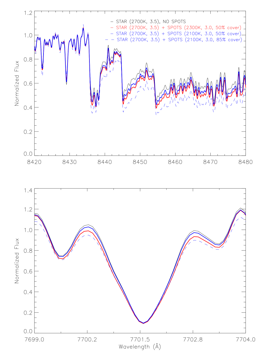
Figure 4: Trends in TiO (top panel) and KI (bottom panel) for spotted photospheres with varying spot temperature and areal coverage. For all models in both panels, the unspotted photosphere has $T_{\rm eff}$ = 2700K and $\log g$ = 3.5, while the spots have an effective gravity of 3.0. In both panels, the black solid line shows the unspotted model; the red solid line shows the model with [T_SPOT, coverage] = [2300K, 50%]; the blue solid line shows the model with [T_SPOT, coverage] = [2100K, 50%]; and the blue dashed line shows the model with [T_SPOT, coverage] = [2100K, 85%]. We see that the [2300K, 50%] spot model is deeper in TiO and broader in Ki than the unspotted case, but the 2100K spot model with the same areal coverage of 50% has reversed in strength, and is closer to the unspotted case than the 2300K model. Increasing the areal coverage of the 2100K case to 85%, however, makes it significantly deeper in TiO and broader in KI than both the unspotted and 2300K spotted models. These changes illustrate the spot-related trends discussed in §6.3. This figure is shown in color in the electronic version only.

In light of this, we investigate the effects of cool spots on our spectra. A priori, the following trends are expected. First, since the spots are by definition cooler than the unspotted photosphere, the TiO bandheads arising inside them will be deeper (relative to the continuum) than those from the surrounding photosphere; the resultant average TiO in a spatially unresolved spectrum will then imply a temperature intermediate between that of the spotted and unspotted surfaces. This trend will not however be monotonic with decreasing spot temperature, since the continuum flux from spots also falls with the spot temperature: the spot TiO contributes less to the average TiO as the spot gets cooler. Thus, for a fixed unspotted photospheric $T_{\rm eff}$ and spot coverage, the average TiO in the combined spotted$+$unspotted spectrum first deepens (relative to the TiO from an unspotted surface) with decreasing spot temperature, and then reverses as the spots become still cooler, to become shallower again (i.e., approaches again the TiO from an unspotted surface). The spot temperature at which this reversal occurs, and thus the maximum depth of the TiO bandheads in the presence of spots, is determined by both the unspotted photospheric $T_{\rm eff}$ and the spot coverage assumed. As an extreme example, 0 K spots contribute no flux at all, and hence, for any coverage $<$100%, will have no effect on the shape of the TiO, which arises in this case only from the unspotted surface (even though the absolute flux in the continuum and bandheads will be lower than in the absence of spots, since the unspotted surface now covers only a fraction of the total stellar surface). The trend in TiO with changing spot temperature and coverage is illustrated in the top panel of Fig. 4.

Second, inside a spot, magnetic fields provide partial support against the external photospheric gas pressure; consequently, the gas pressure alone within a spot is lower than in the surrounding unspotted surface (e.g., Amado et al., 1999, 2000). This exactly mimics the reduction of gas pressure caused by lower surface gravity, and causes the gravity- (more accurately, gas-pressure-) sensitive alkali absorption lines (e.g. K I) in a cool spot to be narrower than outside, thereby implying a lower effective gravity within the spot. The averaged alkali lines in the combined spotted$+$unspotted spectrum will then imply a gravity intermediate between the true photospheric value and the effective one in the spot. Conversely, spots are also cooler than the external photosphere; this tends to make the alkali lines, which are temperature-sensitive as well, broader within a spot, mitigating the narrowing caused by the magnetic pressure effects and reducing the apparent gravity offset. Finally, both effects are limited by the decreasing flux from a spot with lower temperature, exactly as discussed above for TiO; for a given unspotted photospheric $T_{\rm eff}$ and spot coverage, the shape of an alkali absorption line is negligibly changed, relative to that from an unspotted surface, once the spot temperature falls below a certain threshold. The trend in KI with changing spot temperature and coverage is illustrated in the bottom panel of Fig. 4.

These trends have the following consequences. As we have shown, the maximum depth of the TiO bandheads in the presence of spots is determined by both the unspotted photospheric $T_{\rm eff}$ and the spot coverage adopted. Thus, for an observed TiO band depth, specifying the unspotted photospheric $T_{\rm eff}$ sets a lower limit to the spot areal coverage: if the coverage is below this value, the average TiO band depth reverses before it can match the observed depth regardless of how cold the spots become. For a coverage higher than this threshold and fixed unspotted photospheric $T_{\rm eff}$, there is a degeneracy between spot temperature and coverage: a larger coverage allows cooler spots. At the same time, if we decrease the spot temperature we must also decrease the spot’s effective gravity in order to match the observed alkali absorption lines, given the competing effects of gravity and temperature in these lines.

These trends imply that, with a priori knowledge of the unspotted $T_{\rm eff}$, and the true stellar gravity as well as the effective gravity within a spot, one can solve for the spot temperature as well as covering fraction via simultaneous analysis of the TiO and alkali absorptions. We however only know the stellar gravity, and have no advance knowledge of either the unspotted photospheric $T_{\rm eff}$ or the spots’ effective gravity. As such, we can make no claims to a unique solution, or to a full search of the available parameter space. Instead, our goal is a plausible solution, based on constraints set by known properties of sunspots and starspots in general as well as by the 2M0535 lightcurve analysis so far. In particular, we assume that the spots are cooler than the surrounding photosphere by at most $\sim$10–25% (e.g., G09; Linsky et al., 2002), and that the differential between their effective gravity and the higher photospheric value ($\log g$=3.5) is $\lesssim$ 0.5 dex (e.g., Amado et al., 1999, 2000). The unspotted photospheric $T_{\rm eff}$ is also kept a free parameter, but with a lower bound of 2500K set by the $T_{\rm eff}$ inferred from the TiO fits in §5 (the reason for this lower bound is that, if the unspotted photosphere $T_{\rm eff}$ were $<$ 2500K, then combining it with spots that are by definition even cooler could never produce TiO bands that appear to be at 2500K when compared to unspotted models).

Within these constraints, we construct star$+$spot models by assigning synthetic spectra to the unspotted and spotted surfaces, as detailed in §4. We find a viable solution for our spectroscopic data with the following parameters: an unspotted stellar surface with $T_{\rm eff}$ = 2700K and (empirically determined) $\log g$ = 3.5, combined with 70% axisymmetric areal coverage by spots with a temperature of 2300K and effective $\log g$ = 3.0 (i.e., 15% cooler, and 0.5 dex lower apparent gravity, than the unspotted surface).

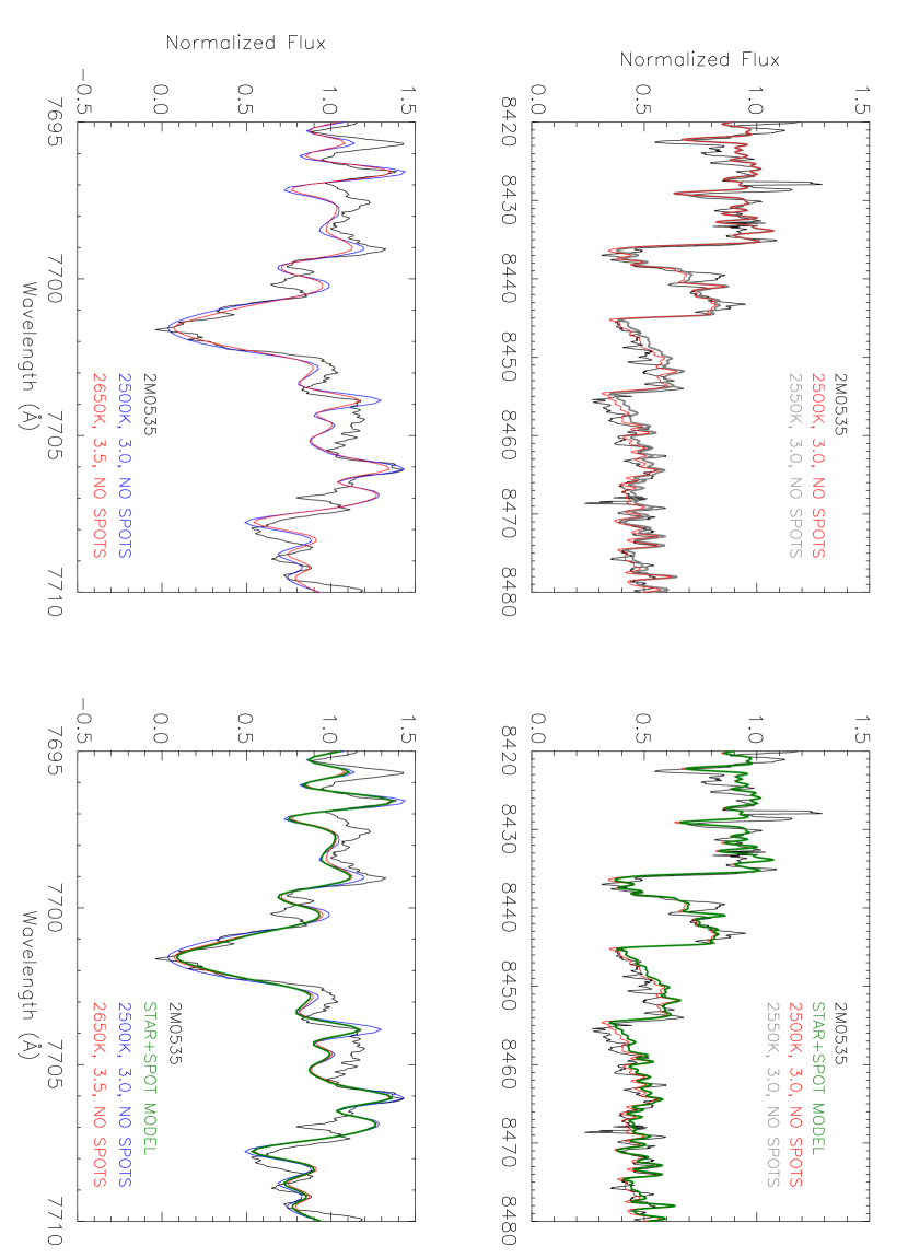
Figure 5: Data for 2M0535A (black) compared to unspotted models (left panels) and a star+spot model (right panels). The TiO comparisons are shown at the top and the K I comparisons at the bottom. The unspotted models plotted are the same best-fit ones plotted in Figs. 1 and 2 (one best-fit model for TiO (in red), two for K I (in red and blue)). Additionally, we plot a 2550K model (in grey) for TiO, to illustrate our adopted error bar of 50K in the $T_{\rm eff}$ derived from TiO. The spotted model (in green in the right panels) is a [2700K, $\log g$ = 3.5] photosphere with [2300K, log $g$ = 3.0] spots covering 70% of the surface. The fits to the spotted model are nearly indistinguishable from the fits to the unspotted models (specifically, the spotted model is an excellent match to the 2550K unspotted model in TiO, i.e., within our adopted $T_{\rm eff}$ error bar for TiO, and to the [2650K, $\log g$ = 3.5] unspotted model in KI), implying that the spotted model is as good a description of the data as the unspotted ones. See §6.3. This figure is shown in color in the electronic version only.

Fig. 5 demonstrates the viability of this spotted model. In the left panels, we compare the data (in black) to the best-fit unspotted models from Figs. 1 and 2 (TiO: best-fit $T_{\rm eff}$ of 2500K [in red], as well as 2550K [in grey] to show the deviation caused by our adopted 50K uncertainty; KI: best-fit $\log g$ = 3.0 at the 2500K implied by TiO [in blue], as well as best-fit $T_{\rm eff}$ = 2650K at the empirically determined $\log g$ of 3.5 [in red]). In the right panels, we compare the best-fit spot model described above (in green) to both the data and the best-fit unspotted models from the left panels. We see that the spotted model very closely reproduces the data as well as the unspotted model fits (in particular, the spotted model is identical to the 2550K unspotted model in TiO, i.e., within 50K – our adopted error – of the best-fit 2500K unspotted TiO model; it is also nearly indistinguishable from the 2650K KI model at the empirical gravity of $\log g$ = 3.5).

Thus, the discrepancies in $T_{\rm eff}$ and $\log g$ implied by the unspotted model-fits to TiO-$\epsilon$ and K I are resolved by this single star+spot model. Consequently, cool spots are a viable explanation for our data.

7 Summary and Conclusions

We have shown that the TiO-$\epsilon$ and K I absorption features in the high-resolution optical spectrum of the higher-mass primary in 2M0535 (2M0535A) are consistent with a $T_{\rm eff}$ = 2700K, (empirical) $\log g$ = 3.5 photosphere combined with cool spots with a temperature of 2300K and effective gravity of $\log g$ = 3.0 covering 70% of the brown dwarf’s surface. This is in agreement with the scenario outlined by CGB07, wherein the temperature reversal in the primary relative to the secondary is caused by magnetic fields, which induce both a reduction in the convective efficiency and high cool spot coverage. While the extreme spot covering fraction we find is similar to that inferred by CGB07 (50% using unrealistic 0 K spots) and G09 (65% with more realistic spots 10% cooler than the photosphere), this very high fraction is nevertheless troubling: in effect, it makes 2M0535A appear to be a “very cool” (2300K) star covered by hot spots, rather than the reverse. On the other hand, we note that Stauffer et al. (2003) argue that the anomalous colours of Pleiades K and M dwarfs result from axisymmnetrically distributed cool spots with a very large areal coverage, $\geq$ 50%; Gullbring et al. (1998) have argued for similarly large axisymmetric spots, with covering fractions of $\sim$ 50–70%, to account for the anomalous colors of even younger weak-lined T Tauri stars (WTTS). There is also evidence for the presence of such axisymmetric large spots from Doppler imaging of WTTS, e.g., large polar spots in V410 Tau (Hatzes 1995) and HDE 283572 (Joncour et al. 1994). Thus, such spots may be usual during the early evolution of these stars, when they are rapidly rotating and highly active, and the phenomenon may extend into the substellar regime as well.

The other option, which we show our results are also consistent with, is that the synthetic spectra are in error, leading to a discrepancy between the $T_{\rm eff}$ and $\log g$ derived from simultaneous fits to TiO-$\epsilon$ and K I (which then leads us to postulate a surfeit of cool spots). R05 postulated such synthetic spectrum errors, also seen in analyses of field dwarfs, to arise from problems with the model TiO-$\epsilon$ oscillator strengths. As we were submitting this paper, it came to our attention that the model errors may lie in the adopted equation of state instead, and that newer models rectifying this are being prepared (A. Reiners & P. Hauschildt, private comm., 2009). Whether these models can resolve the discrepant values obtained from TiO-$\epsilon$ and K I in the case of the very young 2M0535A, without having to resort to copious cool spots, remains to be seen.

Regardless of whether the new models fare better or not, setting rigorous constraints on both the models and the physical conditions on 2M0535A—i.e., determining whether the model fits (and thus the implied $T_{\rm eff}$ and effective log $g$ for the spots) are truly valid and/or if very large cool spots exist on the primary—now requires independently carrying out exactly the same analysis for the lower-mass secondary (2M0535B). CGB07’s theory predicts that the secondary should be much less spotted than 2M0535A: thus, if the same discrepancies between TiO-$\epsilon$ and K I appear in the secondary as well, then errors in the models will be clearly implied; if not, then the suggestion that the primary has an extremely large spot covering fraction will be bolstered. We are currently undertaking observations of 2M0535B to carry out this test.

Finally, if it turns out from 2M0535B’s analysis that the current models are in error (i.e., if the same discrepancies between TiO and K I appear in 2M0525B as well even though it is expected to be relatively unspotted), and thus there is no observational rationale for suggesting very large cool spots on the primary component 2M0535A, then the cause of the temperature reversal between the two binary components once again becomes an unresolved issue. In that case, it may be that the theory proposed very recently by MacDonald & Mullan (2009)—wherein magnetic fields are again to blame, but by inhibiting the onset of convection (though not completely) throughout the star, instead of just in the uppermost super-adiabatic layers as in the theory of CGB07—may be the correct one. Again, we stress that this can only be tested via comparison with an analogous analysis of 2M0535B. Finally, complementary high-resolution spectroscopic observations in the near-infrared (NIR) can be very useful in determining the properties of cool brown dwarfs (e.g. Zapatero Osorio et al., 2006; McLean et al., 2007; Del Burgo et al., 2009), as brown dwarfs are brightest in the NIR. This would be particularly useful for a comparative analysis for the 2M0535 system, where there is a more favorable contrast ratio between the secondary and the primary in the NIR; it would also be helpful for assessing the importance of cool spots, whose influence is less marked in the NIR than in the optical.

This binary, the first eclipsing system in the substellar domain, has already proved to be a rich testing ground for theories of brown dwarf formation and evolution, and it promises to continue being a Rosetta Stone in this regard.

Figure 3: Determination of goodness-of-fit and formal fit parameter uncertainties. Contours of constant $\chi^{2}-\chi_{\rm min}^{2}=$ 2.3,6.2,11.8, representing 1,2,3-$\sigma$ joint confidence intervals in the $T_{\rm eff}$–$\log g$ parameter plane. Top: Joint confidence intervals for fitting of K I. The absolute minimum $\chi^{2}$ best fit is for $T_{\rm eff}=2850$ K and $\log g=4.0$, however a second equally good fit within 1-$\sigma$ confidence occurs at $T_{\rm eff}=2650$ K and $\log g=3.5$. Bottom: Joint confidence intervals for fitting of TiO. The contours demonstrate that for TiO the best fitting model spectra are relatively insensitive to $\log g$ but highly sensitive to $T_{\rm eff}$; a best-fit $T_{\rm eff}=2500\pm 50$ is strongly preferred at high confidence.

References

- Allard et al. (2000) Allard, F., Hauschildt, P. H., & Schwenke, D. 2000, ApJ, 540, 1005
- Allard et al. (2001) Allard,F., Hauschildt,P.H., Alexander,D., Tamanai,A., Schweitzer,A., 2001, ApJ, 556, 357
- Amado et al. (1999) Amado, P. J., Butler, C. J., & Byrne, P. B. 1999, MNRAS, 310, 1023
- Amado et al. (2000) Amado, P. J., Doyle, J. G., & Byrne, P. B. 2000, MNRAS, 314, 489
- Baraffe et al. (1998) Baraffe, I., Chabrier, G., Allard, F., & Hauschildt, P. H. 1998, A&A, 337, 403
- Chabrier et al. (2007) Chabrier, G., Gallardo, J., & Baraffe, I. 2007, A&A, 472L, 17 (CGB07)
- Del Burgo et al. (2009) Del Burgo, C., Martín, E. L., Zapatero Osorio, M. R., & Hauschildt, P. H. 2009, A&A, 501, 1059
- Golimowski et al. (2004) Golimowski, D. A., et al. 2004, AJ, 127, 3516
- Gómez Maqueo Chew et al. (2009) Gómez Maqueo Chew, Y., Stassun, K. G., Prša, A., & Mathieu, R. D. 2009, ApJ, 699, 1196 (G09)
- Gray (1992) Gray, D.F., “The observation and analysis of stellar photopsheres”, 1992, Cambride University Series, vol. 20
- Gullbring et al. (1998) Gullbring, E., Hartmann, L., Briceño, C., Calvet, N., 1998, ApJ, 492, 323
- Hatzes (1995) Hatzes, A. P., 1995, ApJ, 451, 784
- Hauschildt & Baron (1999) Hauschildt, P. H., & Baron, E. 1999, Journal of Computational and Applied Mathematics, 109, 41
- Joncour et al. (1994) Joncour, I., Bertout, C. & Bouvier, J., 1994, A&A, 291, L19
- Jones & Tsuji (1997) Jones, H.R.A & Tsuji, T., 1997, ApJ, 480, L39
- Langhoff (1997) Langhoff, S. R. 1997, ApJ, 481, 1007
- Linsky et al. (2002) Linsky, J. L., Ayres, T. R., Brown, A., & Osten, R. A. 2002, Astronomische Nachrichten, 323, 321
- MacDonald & Mullan (2009) MacDonald, J. & Mullan, D.J., 2009, ApJ, 700, 387
- McLean et al. (2007) McLean, I. S., Prato, L., McGovern, M. R., Burgasser, A. J., Kirkpatrick, J. D., Rice, E. L., & Kim, S. S. 2007, ApJ, 658, 1217
- Mohanty et al. (2004) Mohanty, S., Basri, G., Jayawardhana, R., Allard, F., Hauschildt, P., & Ardila, D. 2004, ApJ, 609, 854 (M04)
- Morales et al. (2008) Morales, J. C., Ribas, I., & Jordi, C. 2008, A&A, 478, 507
- Mohanty et al. (2009) Mohanty, S., Stassun, K. G., & Mathieu, R. D. 2009, ApJ, 697, 713 (MSM09)
- Partridge & Schwenke (1997) Partridge & Schwenke, 1997, J. Chem. Phys., 106, 4618
- Reiners (2005) Reiners, A. 2005, Astronomische Nachrichten, 326, 930 (R05)
- Reiners et al. (2007) Reiners, A., Seifahrt, A., Stassun, K. G., Melo, C., & Mathieu, R. D. 2007, ApJ, 671L, 149 (R07)
- Schweitzer (2001) Schweitzer, A., Gizis, J.E., Hauschildt, P.H., Allard, F. & Reid, I.N., 2001, ApJ, 555, 368
- Schweitzer (1996) Schweitzer, A., Hauschildt, P.H., Allard, F. & Basri, G., 1996, MNRAS, 283, 821
- Schwenke (1998) Schwenke, D.W., 1998, Farraday Discuss., 32(6), 27
- Slesnick et al. (2004) Slesnick, C. L., Hillenbrand, L. A., & Carpenter, J. M. 2004, ApJ, 610, 1045
- Stassun et al. (2006) Stassun, K. G., Mathieu, R. D., & Valenti, J. A. 2006, Nature, 440, 311 (SMV06)
- Stassun et al. (2007) Stassun, K. G., Mathieu, R. D., & Valenti, J. A. 2007, ApJ, 664, 1154 (SMV07)
- Stassun et al. (2008) Stassun, K. G., Mathieu, R. D., Cargile, P. A., Aarnio, A. N., Stempels, E., & Geller, A. 2008, Nature, 453, 1079
- Stauffer et al. (2003) Stauffer, J. et al., 2003, AJ, 126, 833
- Zapatero Osorio et al. (2006) Zapatero Osorio, M. R., Martín, E. L., Bouy, H., Tata, R., Deshpande, R., & Wainscoat, R. J. 2006, ApJ, 647, 1405