Testing for Evolution Using New Type Ia Supernovae
Spectra from the Supernova Legacy Survey

Abstract

GMOS optical long-slit spectroscopy at the Gemini-North telescope was used to classify targets from the Supernova Legacy Survey (SNLS) from July 2005 and May 2006 – May 2008. During this time, 95 objects were observed. Where possible the objects’ redshifts ($z$) were measured from narrow emission or absorption features in the host galaxy spectrum, otherwise they were measured from the broader supernova features. We present spectra of 68 confirmed or probable SNe Ia from SNLS with redshifts in the range $0.17\leq z\leq 1.02$. In combination with earlier SNLS Gemini and VLT spectra, we used these new observations to measure pseudo-equivalent widths (EWs) of three spectral features – Ca ii H&K, Si ii and Mg ii – in 144 objects and compared them to the EWs of low-redshift SNe Ia from a sample drawn from the literature. No signs of evolution are seen for the Ca ii H&K and Mg ii features. Systematically lower EW Si ii is seen at high redshift, but this can be explained by a change in demographics of the SNe Ia population within a two-component model combined with an observed correlation between EW Si ii and photometric lightcurve stretch.

1 Introduction

Since the discovery of cosmic acceleration (e.g. Riess et al. 1998; Perlmutter et al. 1999), Type Ia supernovae have played a vital role as distance measures in the universe, up to and beyond $z=1$ through surveys such as the Supernova Legacy Survey (SNLS Astier et al. 2006) and ESSENCE (Wood-Vasey et al. 2007). This is made possible by the fact that SNe Ia appear to be “standardisable” candles, a property first noted by Phillips (1993) and later parameterised in a number of different ways (for example Riess et al. 1996; Perlmutter et al. 1997; Wang et al. 2003; Guy et al. 2005; Jha et al. 2007). However, the use of the same lightcurve calibration, e.g. stretch, a measure of the relative width of the lightcurve, and colour, at high and low redshift relies on the fact that there is no evolution in the properties of the supernovae with time that cannot be accounted for by the calibration itself.

The properties of high- and low-z objects have been compared in a number of ways. One way is to compare the line profiles and ejection velocities of features in the spectra. Hook et al. (2005) measured the ejection velocity from the blueshifted Ca ii H&K feature in 11 high-z supernovae with $z>0.38$ and compared this to low-z objects. They found that at high-z the ejection velocities and phase evolution of the spectra are consistent with the low-z sample and concluded that there exists a sample at high-z with similar properties to SNe at low-z. Blondin et al. (2006) measured the wavelength of maximum absorption and peak emission for the Ca ii H&K, Si ii 6150 and S ii “W” features and found them to be similar in high-z and low-z objects. They also noted evidence of a double absorption feature in the Ca ii H&K region which is seen to occur occasionally in low-z supernovae and has been attributed to Si ii (Howell et al. 2006).

Since the advent of large surveys producing high numbers of spectra, it has been possible to use these to make composite spectra, which are representative of the average supernovae spectrum in certain redshift and phase bins. This has been done using Keck spectra of SNLS supernovae by Ellis et al. (2008, hereafter E08) with $\overline{z}=0.5$, and for ESSENCE spectra by Foley et al. (2008, hereafter F08). The studies used different methods to account for host galaxy contamination, but neither found definitive evidence for an evolving supernova population. E08 created a composite in order to study possible effects of metallicity variations in progenitors in the rest-frame UV spectra. This is where the absorption is dominated by metal line-blanketing effects and the metallicity differences are expected to be the most prominent, although the theoretical predictions are not in agreement (Höflich et al. 1998; Lentz et al. 2000, for example). E08 saw a large amount of variation in the spectrum in the UV region, more than is predicted and can be accounted for by dust, and also changes with phase that are not predicted. However, due to a lack of local UV spectra of supernovae they are unable to draw any firm conclusions as to evolution.

F08 do not perform galaxy subtraction, but instead contaminate their low-z spectra with a known galaxy spectrum in an attempt to match the host galaxy contamination of their high-z sample. They find evidence of changes in the Fe ii spectral feature which may indicate lower ⁵⁴Fe production in a lower temperature environment brought on by a lower metallicity. They attribute this not to evolution, but to changing demographics as the universe at higher redshift was less metal-rich compared to the universe today; however, again their conclusions are limited by the low-redshift sample of spectra.

The composite spectra from E08 was included in Sullivan et al. (2009) which compared their medium redshift composite to a new low-z composite ($z<0.05$) and a high-z composite ($z>0.9$) based on data from Riess et al. (2007). They observe a clear decrease in the size of spectral features of intermediate mass elements as redshift increases, but this is a change which is consistent with a change in demographics, rather than an evolution of SNe Ia.

Other studies have focussed on measuring the pseudo-equivalent widths of spectral features in the high-redshift spectra and comparing these to trends with phase in the low-redshift sample. This method was first described by Folatelli (2004, hereafter F04) and used successfully on a small sample of spectra to compare low- and high-redshift objects for 5 distinct features in the spectrum. The blueshift of the absorption minimum in Ca ii H&K was also measured and compared to nearby supernovae and no evidence for any significant differences was found between the two samples (see also Garavini et al. 2007).

An EW analysis of the first two and a half years of Gemini SNLS spectra was published in Bronder et al. (2008, hereafter B08). Rest-frame EW measurements were made for the Ca ii H&K, Si ii 4000 (hereafter referred to as just Si ii) and Mg ii features as well as the Ca ii H&K ejection velocity. The spectra of 55 high-z supernovae were compared to 167 spectra from 24 low-z objects encompassing all three SNe Ia sub-types (normal, overluminous and underluminous). No significant difference was seen between the two samples for the equivalent widths of Ca ii H&K and Si ii or the ejection velocity. For the Mg ii feature, a slight difference was noted, but it was not significant enough to confirm evolution and could just have been a statistical effect. This is discussed further in Section 4.4. B08 also found a relation between the EW Si ii and $M_{B}$, the absolute B-band magnitude at maximum, which could be used to calibrate the supernovae in the same way as lightcurve stretch and colour.

With the well-measured light curves of the SNLS supernovae it has also been possible to compare photometric properties. In Conley et al. (2006), the rise-times of low- and high-z supernovae are compared and they find no compelling evidence that there is a difference between the two populations.

However, as was concluded by F08, there is to be expected some change in photometric properties due to changing demographics. Due to the two-channel progenitor model (Scannapieco & Bildsten 2005; Mannucci et al. 2005, 2006; Sullivan et al. 2006), the “prompt” component which are brighter supernovae with broader light curves should dominate at higher redshift, whereas at $z=0$, the “delayed” component will be more important. Howell et al. (2007); Sullivan et al. (2009) calculate that this should result in a 6% increase in light curve width between $z=0$ and $z=1.5$. Using observational data from Sullivan et al. (2006), they measure a percentage change in stretch of $8.1\pm 2.7$% between $0.03<z<1.12$ which is consistent with changing demographics. The spectral evolution observed in Sullivan et al. (2009) is consistent with this.

In summary, no firm evidence of evolution in the spectral properties of supernovae has been observed, but the studies are being hampered by the lack of local spectra to compare with. In this paper we present an analysis of EWs of the Ca ii H&K, Si ii and Mg ii spectral features. This study significantly expands on the work of B08 using new data from SNLS with a different method of accounting for the effects of host galaxy light, as well as an expanded sample of low-z SNe from the literature for comparison.

The remainder of this paper is organised as follows. In section 2 we describe the new observations. In section 3 we detail the methods and measurements applied to the high-z sample of SNe Ia. Section 4 describes the low-z sample drawn from the literature and used for comparison. Section 5 details the results of the comparison study and an investigation into the possible cosmological uses for SNe Ia spectra. These are discussed further in section 6 and our conclusions are summarised in section 7.

2 Observations

The targets were selected from real-time SNLS imaging which took place at the Canada-France-Hawaii Telescope. Fainter objects were usually observed spectroscopically at Gemini, with brighter candidates at either VLT or Keck (see Perrett et al. (in prep.) for more details on the real-time pipeline).

2.1 Observational Set-up

The new spectra presented here were taken in queue mode on the Gemini-North telescope with ToO status. The observational set-ups and data reduction methods used for SNLS-Gemini spectroscopy using GMOS (Hook et al. 2004) have been described in detail previously (Howell et al. 2005; Bronder et al. 2008). In summary, a ’classical’ setup with central wavelength of 680nm was used for observations of brighter targets which were expected to be at a lower redshift, whereas nod-and-shuffle mode (N&S, Glazebrook & Bland-Hawthorn 2001) with a redder central wavelength of 720nm was used for fainter targets. The only change to the methods of observational set-up since Howell et al. (2005, hereafter H05) and B08 are that from March 2007, first N&S and then classical observations were taken at two wavelength settings in order to cover the gaps in the spectra caused by the spacing of the three GMOS CCDs. In these cases, for the R400 grating and with $2\times 2$ binning, the change in central wavelength used was 50 nm. Due to the unavailability of the R400 grating, three targets were observed with the R150 grating which has a lower dispersion. For these objects, a change in central wavelength of 100 nm was used.

The position angle of the slit was primarily determined by aligning the target and the centre of the host galaxy in order to try to observe narrow emission/absorption features in the host spectrum. The second constraint was the availability of guide stars in the field. Occasionally, less optimum position angles were used or the object was moved from the centre of the slit. All of these considerations mean that the observations were not taken at parallactic angle, but this is taken into account in the analysis that follows.

The new targets observed as part of the Gemini SNLS spectroscopic follow-up programme are listed in Table 8.

2.2 Data Reduction

The data were reduced using standard IRAF and Gemini-specific tasks to perform bias-subtraction, flat-fielding, sky-subtraction and chip mosaicing. A wavelength solution was applied to the 2D spectrum. When combining the 2D frames, bad-pixel masks were used to take account of the “missing data” in the gaps between the CCDs. A 1D spectrum was extracted from the 2D spectrum and corrected for telluric absorption features. It was generally not possible to extract the target light separately from the host due to the small angular separation of the objects on the sky. A sky spectrum was also extracted from the 2D frames, and an error spectrum was estimated from this by assuming that the noise is dominated by sky emission. Where appropriate in some of the earlier data which were observed at only one central wavelength, a linear interpolation was used to remove the chip gaps and the error spectra set to a high value in these regions to deweight them.

2.3 Redshift Determination and Object Classification

The redshifts of the supernova and its host are ideally measured using narrow host features such as [O iii], [O ii], H$\beta$ and H$\alpha$ emission, and H&K absorption. This typically gives an error of $z\pm 0.001$, but if many lines are present then the error can be reduced further. If no host features are present then the redshift measurement relies on the wider supernova features. These are less precise due to the higher velocities involved and typically measure $z\pm 0.01$ depending on the quality of the spectrum.

A high-z SN Ia is classified by identifying, typically, the Si ii feature at $\lambda\approx 4000$ Å in the spectra. Other features used are Si ii $\lambda 6150$ and S ii. To aid classification, all spectra are also run through the SUPERFIT program (H05) which performs a $\chi^{2}$-minimisation to best-fit the observed spectra to a low-z supernova spectrum combined with host galaxy light. Objects are classified as SNIa (certain or highly probable Ia), SNIa? (probable Ia), SNII (SN Type II), SN (supernova of unknown type) or SN? (probable SN of unknown type). To go alongside this, spectra are assigned a confidence index (CI) from 0–5 with 5 being a definite Ia and 0 definitely not. Objects of CI = 0 are typically core-collapse supernovae. The definitions of the CIs are given in H05.

The redshifts, their errors and CIs of all the objects observed in this study are given in Table 11.

2.4 Sub-Type Identification

A number of SNe Ia were observed to have spectral features similar to known peculiar objects from their best-fit SUPERFIT matches (H05). Identification of these objects is important so they can be flagged and removed from later studies. The objects which were identified as having unusual spectral features during this period of observation are given in Table 1.

There are several key features which are distinct to each of the comparison spectra. SNLS-03D3bb (SN 2003fg Howell et al. 2006) was an overluminous SNe Ia whose progenitor system is debated, but it is thought to be of super-Chandrasekhar mass. The spectrum showed low ejection velocities, as well as an unburnt C ii feature at 4200Å. SN 2001ay (Howell & Nugent 2004) has a high stretch value ($s=1.6$), but appeared spectroscopically normal around maximum light, except for high-velocity Ca ii and Si ii features. SN 1999aa (Garavini et al. 2007) has been seen as a transitional object between normal SNe Ia and the overluminous objects typified by SN 1991T (Filippenko et al. 1992), showing spectral features of both types of object. SN 1999aa spectra at maximum contained smaller amounts of intermediate mass elements and larger amounts of iron-group elements, and appeared peculiar until maximum light after which it appeared to be spectroscopically normal.

Table 1: Unusual SNe Ia identified in this sample from their spectral features only. The stretch measurements are made using the SiFTO (Conley et al. 2008) light curve fitter. The references for the comparative objects are SNLS-03D3bb (Howell et al. 2006), SN 2001ay (Howell & Nugent 2004) and SN 1999aa (Garavini et al. 2004).

Object	Stretch		Comments
07D3af	0.943 $\pm$	0.017	03D3bb-like
			C ii feature at 4200Å
07D3ap	0.955 $\pm$	0.018	SN 2001ay-like
			High-velocity Si ii
07D3cr	0.872 $\pm$	0.043	SN 2001ay-like
			Broad Ca ii
07D3dj	1.118 $\pm$	0.018	03D3bb- or SN 1999aa-like
			Little Ca ii and probable C ii
08D2aa	1.128 $\pm$	0.016	SN 1999aa- or SN 2001ay-like
			C ii feature at 4200Å
08D2ad	1.155 $\pm$	0.021	03D3bb-like
			C ii feature at 4200Å

3 Methods and Measurements

For the use of SNe Ia as cosmological distance indicators, it is important to verify that the objects we observe in the high-z universe have similar properties to those at low z, or, if there is some change in the mean properties (Howell et al. 2007, for example), that these differences can be calibrated out. All previous work on high-z SNe Ia spectra (e.g. Hook et al. 2005; Blondin et al. 2006; Ellis et al. 2008; Bronder et al. 2008; Foley et al. 2008) have found no definitive evidence for evolution beyond what is expected from known changes in demographics.

In this paper out of the 95 objects observed, 68 were confirmed as Type Ia or probably Type Ia events. Previous Gemini SNLS samples have published a further 41 (H05) and 46 (B08).

3.1 Sample Selection

For the study here, all SNLS supernovae observed with Gemini, including objects published in H05 and B08, with confidence indices of 4 or 5 were considered. A cut was then made based on the availability of final lightcurves and measurements of conditions on the night of observation, specifically hour angle (HA) and mean seeing. The HA and seeing are required for light-loss correction described in Section 3.3.3. In the case of observations spread over more than one night, the larger value of the seeing was used.

A comparison sample of spectra drawn from the first three years of SNLS-VLT spectra analysed in real-time (Basa et al. in prep) was also used. These objects were observed using the FORS1 spectrograph (Appenzeller et al. 1998) on the VLT. Again, these objects were required to have CI=4 or 5 and have final lightcurves and a measurement of seeing for the EW study. In this case, the measurements of the hour angle on the night of observation were not required as FORS1 employs an atmospheric dispersion correction (ADC) which minimises the amount of light lost when not observing at the parallactic angle.

Removing objects classified as peculiar (see Table 1), the sample for the EW study contains 149 objects, 82 from Gemini and 67 from the VLT. A histogram of redshift is shown for the final Gemini and VLT samples in Figure 1. It shows that the Gemini sample peaks at a higher mean redshift, as expected since Gemini was used to observe the candidates that were expected to be at higher redshift, but also contains a larger number of lower redshift objects than the VLT sample. These are objects from the D3 field which is not visible in the southern sky. The mean redshifts illustrated by the dotted line are $\overline{z}_{Gem}=0.63$ and $\overline{z}_{VLT}=0.60$. The median of the VLT sample is similar to its mean, but for the Gemini sample, due to the large number of points at $z>0.8$ has a median value of $0.70$.

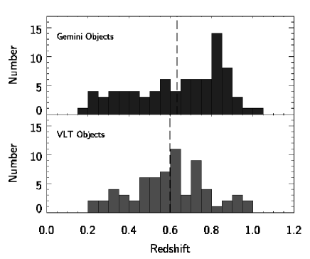
Figure 1: Redshift histogram for the Gemini and VLT samples. The dotted line represents the mean redshifts of the two samples.

3.2 Photometric Data and Host Galaxy Template Fitting

For this study, SNLS multicolour photometry of the supernovae and their host galaxies was used for two main purposes: firstly for subtraction of the host galaxy contamination from the spectra; and secondly, for comparison of spectral features with photometric properties of the supernovae.

The photometric lightcurve data for the high-z SNLS sample above, and the low-z comparison sample described in Section 4, was fitted using the SiFTO lightcurve-fitter (Conley et al. 2008) to ensure homogeneity in the sample. This provided measurements of lightcurve stretch, colour and date of maximum. It also permitted the interpolation of supernova magnitudes in $g^{\prime}r^{\prime}i^{\prime}z^{\prime}$-bands to the date of spectroscopic observation.

From stacked images, the host galaxy surface brightness in $u^{*}g^{\prime}r^{\prime}i^{\prime}z^{\prime}$-bands at the position of the supernova was measured. These were used to find a best-fitting galaxy template spectrum. The same template library as in E08 was used, which was drawn from the PÉGASE programme (Fioc & Rocca-Volmerange 1997, 1999), and a star-burst template (SB1) from Calzetti et al. (1994) was added. Emission-line features were interpolated over.

A $\chi^{2}$ minimisation was used to compare synthetic photometry from the templates in the $u^{*}g^{\prime}r^{\prime}i^{\prime}z^{\prime}$-bands, $f_{temp,i}$ to the measured values $f_{gal,i}$ by minimising

$$\chi^{2}=\sum_{i}{\frac{(f_{gal,i}-(A\lambda+B)f_{temp,i})^{2}}{\sigma_{gal,i}^{2}}}$$ (1)

where $\sigma_{gal,i}$ is the error on the galaxy flux in band $i$. The template is normalised by the function $A\lambda+B$ to allow for reddening in the host galaxy. The best-fit galaxy template $(A\lambda+B)f_{temp}$ is denoted below as $f_{g}^{bf}(\lambda)$.

3.3 Galaxy Subtraction Method

Here we use a galaxy subtraction method similar to the one described in E08, rather than the correction factor method in B08, but with one large difference. The objects observed as part of the E08 study were all observed at parallactic angle where supernova light-loss from the slit was minimised whereas in this study the observations were not taken at parallactic angle. In order to carry out a galaxy subtraction, we assume the galaxy is a flat background and the supernova is modelled as a point-source with a FWHM equal to the seeing in the band used for object acquisition (either r^′ or i^′), and scaling with wavelength as $\lambda^{-0.2}$. Under this assumption, light from the supernova will be lost due to atmospheric differential refraction (ADR). We account for this in Section 3.3.3.

The galaxy subtraction method is summarised in the following sections.

3.3.1 Correcting To Compensate For Different Observing Conditions

Starting with the raw spectrum, $f_{tot}^{raw}(\lambda)$, which is the sum of supernova flux, $f_{SN}^{raw}(\lambda)$, and galaxy flux, $f_{g}^{raw}(\lambda)$, the aim is to produce a final corrected supernova spectrum, $f_{corr}(\lambda)$.

The SNLS observations were not spectrophotometric, therefore before the galaxy template (which is normalised to SNLS host photometry) can be subtracted, the observed spectrum must be placed on the same flux scale. This is done by multiplying by a correction factor $A_{sens}$ calculated by comparing photometry of the supernova and host from the imaging, correctly scaled to match observing conditions and observational set-up, to the synthetic $r^{\prime}$- and $i^{\prime}$-band flux in the observed spectrum. $A_{sens}$ is the mean of the corrections needed to match the $r^{\prime}$- and $i^{\prime}$-band flux.

$$f_{tot}(\lambda) = f_{tot}^{raw}(\lambda)\times A_{sens}$$

We denote the photometrically-normalised SN and host galaxy spectra as

$$f_{SN}^{s}(\lambda) = f_{SN}^{raw}(\lambda)\times A_{sens}$$

$$f_{g}^{s}(\lambda) = f_{g}^{raw}(\lambda)\times A_{sens}.$$

3.3.2 Template Subtraction

The fractional contamination (FC) of galaxy light in the total spectrum is calculated for both the $r^{\prime}$- and $i^{\prime}$ bands using the galaxy and SN photometry and accounting for the effects of the observing conditions. Any object with fractional contamination of galaxy light in the total spectrum $FC\geq 0.1$ in either band has the best-fitting galaxy template subtracted-off. The FC is calculated in two bands instead of one because as it is measured in the observed frame, there will be a redshift-dependence on the value of FC as the filters will fall at different points in the rest-frame of the object. In situations with $z<0.7$, the $i^{\prime}$-band filter falls in the redder part of the spectrum where there is less supernova flux relative to galaxy; and at $z>0.7$, the reverse is true. The FC will also be phase-dependent as the supernova spectrum becomes redder with time. The value of $0.1$ was chosen because at this level of contamination, the error on the EW measurements will be $\approx$10%, which is comparable to the size of the error introduced by misidentifying the galaxy host type (see Section 3.5). Also, below this level of contamination, the risk of subtracting too much galaxy template is high.

Before subtraction can occur, the best-fit galaxy template, $f_{g}^{bf}(\lambda)$, must be scaled to account for differences between the photometry apertures and the spectroscopy apertures. The galaxy photometry is in units per square arcsecond (or effectively in an aperture of size $1^{\prime\prime}\times 1^{\prime\prime}$). The aperture size of the spectroscopy is given by the slit width, which is always $0.75^{\prime\prime}$ for GMOS observations, but varies for the VLT spectra, multiplied by the size of the aperture window used during extraction, and is denoted by $A_{ap}$ in units of square arcseconds. Under the assumption of a flat host galaxy background, the flux of the host transmitted through the slit, $f_{g}^{t}(\lambda)$, is then

$$f_{g}^{t}(\lambda) = f_{g}^{bf}(\lambda)\times A_{ap}$$

The galaxy template is then interpolated to the same wavelength scale as the observed spectrum and subtracted off leaving the intermediate step

$$f_{corr}^{int1}(\lambda) = f_{tot}(\lambda)-f_{g}^{t}(\lambda)$$

$$= f_{SN}^{s}(\lambda)+f_{g}^{s}(\lambda)-f_{g}^{t}(\lambda).$$

In an ideal situation, where the galaxy template matches the observed galaxy perfectly, $f_{g}^{s}=f_{g}^{t}$ leaving a spectrum containing only supernova flux.

3.3.3 Correcting for ADR

The spectrum now contained only supernova light, but the colours were not correct due to the loss of light at the wavelengths not used for acquisition. See Filippenko (1982) for the equations governing light loss as a function of wavelength, hour-angle, seeing, airmass etc.. A correction function, $c_{ADR}(\lambda)$, for the supernova spectrum was found by fitting a second-order polynomial to the inverse of the fraction of SN light which is transmitted through the slit at the effective wavelength of each band, i.e. multiplication by $c_{ADR}(\lambda)$ should have corrected the spectrum so it represented the total supernova flux. The fitting was calculated using MPFITFUN, part of MPFIT (Markwardt 2008). The final, subtracted, ADR-corrected spectrum, $f_{corr}(\lambda)$, was given by:

$$f_{corr}^{int2}(\lambda) = (f_{SN}^{s}(\lambda)+f_{g}^{s}(\lambda)-f_{g}^{t}(\lambda))c_{ADR}(\lambda).$$

Note that this correction was not applied to the VLT spectra.

3.3.4 Extinction Correction

The final step is to correct for extinction in both the host galaxy and the Milky Way. In the rest-frame, the SALT2 colour law (Guy et al. 2007), a function of wavelength, redshift and SN colour, is applied to each object to account for the host extinction. This correction is small and has almost no effect on the EW measurements. In the observed frame, the Cardelli, Clayton and Mathis (1989) extinction law is applied to account for Milky Way extinction using the dust maps of Schlegel et al. (1998). The SNLS fields are selected to be in regions with low galactic extinction so the Milky Way correction is not large either. These corrections can be summarised as $c_{ext}(\lambda,z,c)$ where $c$ is the supernova colour.

$$f_{corr}(\lambda) = (f_{SN}^{s}(\lambda)+f_{g}^{s}(\lambda)-f_{g}^{t}(\lambda))c_{ADR}(\lambda)c_{ext}(\lambda,z,c).$$

The final spectrum contains only supernova light and can have the equivalent widths of the features measured.

The same scaling treatment is applied to the error spectrum, but no subtractions are done because it is assumed to contain only sky noise. As an example, the galaxy-subtracted spectrum for 07D3ea is illustrated in Figure 2.

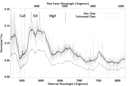
Figure 2: Example of host galaxy subtraction from a high-z SNLS supernova spectrum. The raw data (for object 07D3ea at z=0.471) is shown in light grey, with a smoothed version over the top in black. The SN spectrum after subtraction is shown as the smoothed light grey line underneath. 07D3ea was best-fit by an star-burst galaxy template and has $FC=0.19$ in the $i^{\prime}$-band.

3.4 Equivalent Width Measurements

The equivalent widths were measured in the same way as in B08, fitting a pseudo-continuum to the feature and calculating the EW between these limits. The pseudo-continuum was defined by the highest point in a region either side of the feature. In general, an EW and its associated statistical error are given by:

$$EW = \sum_{i=1}^{N}\Bigg{(}1-\frac{f_{\lambda}(\lambda_{i})}{f_{c}(\lambda_{i})}\Bigg{)}\Delta\lambda_{i}$$ (2)

$$\sigma^{2}_{EW} = \sum_{i=1}^{N}\Bigg{(}\Big{(}\frac{\sigma_{f}(\lambda_{i})}{f_{c}(\lambda_{i})}\Big{)}^{2}+\Big{(}\frac{f_{\lambda}(\lambda_{i})}{f_{c}^{2}(\lambda_{i})}\Big{)}^{2}\sigma^{2}_{c_{i}}\Bigg{)}\Delta\lambda_{i}^{2}$$ (3)

where $f_{\lambda}$ is the flux of the spectrum, $f_{c}$ is the flux of the pseudo-continuum, $\sigma_{f}$ is the uncertainty in the flux from the error spectrum and $\sigma_{c_{i}}$ is the uncertainty in the pseudo-continuum. However, as error spectra were available for the SNLS observations, it was possible to weight each point in the calculation and account for uncertainties in the flux due to sky noise. Equation 2 was modified to:

$$EW_{\mathrm{SNLS}} = \Bigg{(}\sum_{i=1}^{N}\Bigg{(}1-\frac{f_{\lambda}(\lambda_{i})}{f_{c}(\lambda_{i})}\Bigg{)}\Delta\lambda_{i}w_{i}\Bigg{)}\frac{N}{\sum_{i=1}^{N}(w_{i})}$$ (4)

where $w_{i}$ is the weighting of each point given by $w_{i}=\frac{1}{\sigma_{f}(\lambda_{i})^{2}}$. The statistical error was still calculated as given in Equation 3.

The same EW code for measuring the features as in B08 was used with changes to the method used to select the limits of the pseudo-continuum to make the process more automatic. The ranges of wavelength for the blue and red bounds of the SNe Ia features were first defined in F04 and were the ones used in B08. In this study, we used the Ca ii H&K, Si ii and Mg ii features and the boundaries for these features were redefined according to observations of low-z and high-z objects using trial and error to find the optimum values in order to make the process more automated. The new ranges are given in Table 2.

Table 2: The spectral ranges defined in Folatelli (2004) compared to the new ranges defined here.

Feature	Folatelli Blue	New Blue	Folatelli Red	New Red
	Limit (Å)	Limit (Å)	Limit (Å)	Limit (Å)
Ca ii	3500 – 3800	3500 – 3700	3900 – 4100	3900 – 4100
Si ii	3900 – 4000	3900 – 4000	4000 – 4150	4050 – 4125
Mg ii	3900 – 4150	4050 – 4200	4450 – 4700	4450 – 4700

As the definitions of the SNe Ia spectral features in F04 overlap, the code could over-estimate the Ca ii feature or the Mg ii feature by including the Si ii feature. The code now automatically adjusts the ranges to compensate for this depending on the supernova “colour”. As a crude way of calculating this from the spectrum, the ratio of integrated flux in the region 50-100 Å above and below the minimum of the Si ii feature was measured and used to move the boundaries of the features so the over-estimation no longer occurs. For a redder supernova, the red limit of the Ca ii feature was decreased and for a blue supernova, the blue limit of the Mg ii feature was increased.

In the event that the automation still failed, the bounds for the pseudo-continuum had to be selected manually. In this case an error to account for the uncertainty in the placement of the feature bounds was calculated by varying the boundaries within $\pm$10 Å at random and evaluating the EW fifty times. The resulting EWs were fitted with a Gaussian and the pseudo-continuum contribution to the EW error was given by the standard deviation of the Gaussian. This was added in quadrature to the statistical error.

The EW measurements for the 149 objects in the final sample are in Tables 13, 14 and 15. At this point, five objects were removed from the sample as the galaxy subtraction method was believed to have failed for these objects. This was reflected in either negative values of EWs or values of EW Mg ii close to 0. These objects tended to occur in the very centre or on the outskirts of the host where the assumption that the host contribution does not vary within the size of the spectroscopy aperture. The objects are marked with an * in the results tables. This left a total of 144 objects: 78 objects from the Gemini telescope and 66 from the VLT.

3.5 Evaluation of Additional Sources of Error

Using the multicolour host galaxy subtraction method there are several extra terms in the error calculation as well as the statistical error. Firstly, there is an uncertainty in the selection of the galaxy template. Any galaxy template within a $3\sigma$ range of the best-fit galaxy is identified to rule out any galaxy template which is definitely not the host. This is illustrated in Figure 3 for the example of 06D1bz above. The best-fitting template is that of an S0 galaxy, but the elliptical and irregular galaxy spectrum lie within the $3\sigma$ range.

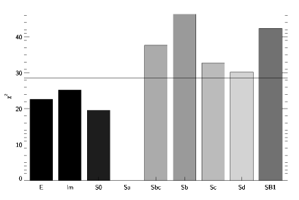
Figure 3: A histogram plotting the minimum $\chi^{2}$ values found for each of the galaxy templates for the photometry of 06D1bz. The best fit is an S0 galaxy, but the elliptical and irregular templates cannot be ruled out. The lower line marks the minimum $\chi^{2}$ and the higher line marks the $3\sigma$ region. There is no $\chi^{2}$ value for the Sa template as this fit does not converge.

Any galaxy template fit falling within this $3\sigma$ range are appropriately scaled, subtracted from the raw spectrum and the EW measured. The scatter in EW measurements is then used to produce an error due to misidentification of the galaxy type. It is typically in the order of a few Å (i.e. 10% EW) and is added in quadrature to the $1\sigma$ statistical error from the EW measurement.

Another change from B08 is that measurements of EW features where a GMOS chip gap has fallen in the boundary regions of the feature are no longer removed from the sample. Instead, a linear interpolation is made across the gap. The presence of the chip gap adds to the error on the EW measurement as there is no data in that region. To compensate for this, the statistical error is increased by a multiplicative correction factor $A_{gap}$ to take into account the number of pixels which form the feature where there is essentially no information.

$$A_{gap} = \sqrt{\frac{N_{tot}}{N_{tot}-N_{gap}}}$$

where $N_{tot}$ is the total number of pixels in the feature and $N_{gap}$ is the number of pixels from the chip gap included in that feature.

4 Low-z Comparison Sample

4.1 Spectroscopy Sample

The equivalent widths of the Ca ii H&K, Si ii and Mg ii features change with the phase of the supernova so it is important to find a sample with good phase coverage. In order to select a sample, the SUSPECT archive was used to search for published spectra with phases of $\pm 11$ days from B-band maximum. This phase range was chosen to match the range of rest-frame phases in the high-z spectra. Before $-11$ days spectra are rare because of the time needed to discover the objects and arrange spectroscopy scheduling. After $11$ days, there are not many high-z spectra as the supernovae have faded. The selection criteria applied to the spectra were: that there should be at least two spectra within the $\pm 11$ day range as we want to study the evolution of spectra features with time; the spectra should include all three of the Ca ii H&K, Si ii and Mg ii  features so as to be certain the supernovae are normal in the whole region being investigated; all the objects should be classified as core-normal supernovae.

There are a number of problems with applying these criteria to the current low-z sample. Firstly, a lot of published spectra do not have the wavelength coverage to include the Ca ii H&K feature as this is in the near-UV which is difficult to observe from the ground. Secondly, the well-studied objects tended to be the spectroscopically or photometrically peculiar examples which are not useful for this study.

Applying these criteria to the SUSPECT archive produced 104 spectra from 14 objects. This was then combined with 49 spectra from 11 objects published in Matheson et al. (2008); however, the latter objects are excluded from the analysis of the Ca ii H&K feature. This is because the spectrograph used has a blue limit of 3700 Å which would mean the feature would only be completely visible in spectra of objects with a narrow Ca ii feature at certain redshifts and so bias the sample. Table 3 details the 23 low-z objects used in this study.

Table 3: Low-z sample used to make the low-z trends. Objects with published photometry are marked with a ^† symbol. Objects in galaxies with known distance moduli or within the Hubble flow ($z\geq 0.2$) are marked with a ^‡. Five objects have been used in the low-z cosmology sample in Astier et al. (2006) and these are marked with an $\ast$.

Supernova	Phases of Spectra Used	Reference
SN 1989B †‡	$0$,$6$,$11$	Barbon et al. (1990)
SN 1990N †‡	$-8$	Leibundgut et al. (1991)
	$2$	Mazzali et al. (1993)
SN 1994D†‡	$-11$,$-10$,$-9$,$-8$,$-5$, $-4$,$-2$,$2$,$4.10$,$11$	Patat et al. (1996)
SN 1996X †	$-2$,$0$,$1$,$7$	Salvo et al. (2001)
SN 1998aq †‡	$-9$,$-8$,$1$,$2$,$3$,$4$,$5$,$6$,$7$	Branch et al. (2003)
SN 1998bu †‡	$-4$,$-3$,$-2$,$8$,$9$,$10$,$11$	Jha et al. (1998)
SN 1999ee †	$-11$,$-9$,$-4$,$-2$,$0$,$5$, $7$,$9$	Hamuy et al. (2002)
SN 2000E †	$-9$,$-6$,$-5$,$5$	Valentini et al. (2003)
SN 2002bo †	$-11$,$-6$,$-5$,$-4$,$-3$, $-2$,$-1$,$4$	Benetti et al. (2004)
SN 2002er †	$-11$,$-9$,$-8$,$-7$,$-6$, $-5$,$-4$,$-3$,$-2$,$-1$,$0$, $2$,$4$,$5$,$6$,$10$	Kotak et al. (2005)
SN 2003du †	-11,-7	Anupama, Sahu & Jose (2005)
	$-8$,$-6$,$-4$,$-2$,$-1$,$0$, $1$,$3$,$4$,$7$,$8$,$9$,$10$	Stanishev et al. (2007)
SN 2004S †	$1$,$7$	Krisciunas et al. (2007)
SN 2004dt	$-10$,$-9$,$-7$,$-6$,$-4$, $-3$,$-2$,$-1$,$2$,$3$	Altavilla et al. (2007)
SN 2004eo †	$-6-3$,$2$,$7$,$11$	Pastorello et al. (2007)
SN 1997do †	$-11$,$-10$,$-7$,$-6$,$9$,$11$	Matheson et al. (2008)
SN 1998V †$\ast$	$1$,$2$,$3$	Matheson et al. (2008)
SN 1998dh †	$-9$,$-8$,$-7$,$-5$,$-3$,$0$	Matheson et al. (2008)
SN 1998ec †‡	$-3$,$-2$	Matheson et al. (2008)
SN 1998eg †‡$\ast$	$0$,$5$	Matheson et al. (2008)
SN 1999cc †‡$\ast$	$-3$,$-1$,$1$,$2$	Matheson et al. (2008)
SN 1999ej	$-1$,$3$,$5$,$9$	Matheson et al. (2008)
SN 1999gd †	$3$,$10$	Matheson et al. (2008)
SN 1999gp †‡$\ast$	$-5$,$-2$,$1$,$3$,$5$,$7$	Matheson et al. (2008)
SN 2000fa †‡$\ast$	$-10$,$2$,$3$,$5$,$10$	Matheson et al. (2008)
SN 2001V †	$-11$,$-10$,$-9$,$-8$,$-7$, $-6$,$-4$,$9$,$10$	Matheson et al. (2008)

4.2 Photometry Sample

The photometric properties of all 21 supernovae which have published photometry were refitted using the SiFTO light curve fitter to produce a consistently-fitted sample. The lightcurves were fitted for stretch, colour, date of maximum and peak magnitude, which were useful for studying any possible relation between the spectroscopy features and residuals from the Hubble diagram. The results are summarised in Table 16, which also shows any independent distance modulus measurements available for the host.

4.3 Low-z Equivalent Width Measurements and Errors

The EWs were evaluated using Equation 2 and all measurements were made in the object’s rest-frame. The values are given in Table 17. Error spectra were not available for the low-z spectra as they were for the high-z SNLS data which is why Equation 2 was used. This meant that no statistical error on the EW could be measured. The assumption in B08 was that the main source of error was due to incorrectly placing the pseudo-continuum bounds around the features and this error was quantified in the same way as described for the high-z data in Section 3.4; however, the low-z spectra are of high signal-to-noise and, as the equivalent width measurement code had been made much more automated, these errors were negligible. When one measurement of the EW was required per supernova, the mean over all epochs was measured and the error was assigned based on the RMS scatter about the mean. This was a good estimation for the features being investigated here as the spectral features appear to be approximately constant with phase within the phase range investigated (see Figure 4).

4.4 Low-Redshift Trends

We calculate low-redshift trends as a measure of the variation of spectral features with phase relative to the date of maximum. The trend is calculated by measuring a resistant median each day $\pm 10$ from B-band maximum. The resistant median removes outliers which are more than $3\sigma$ from the median. The weights applied to each measurement is a Gaussian centered on that date with a FWHM of 4 days. This time-frame was chosen as smaller time intervals result in the trend becoming affected by the scatter of the EW and any poor phase sampling. A weighted RMS was calculated to produce the $1\sigma$ scatter for the sample. The resulting trends are presented in Figure 4.

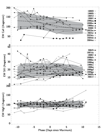
Figure 4: Low-z Trends for Ca ii H&K, Si ii and Mg ii. The individual supernova measurements are marked by the different symbols. The central thick dotted line is the trend and the grey shaded region represents the $1\sigma$ error distribution. The legend applies to all 3 panels.

The trends shown in Figure 4 show that over the range of phases studied, all three features are approximately constant. The Ca ii H&K feature decreases in strength slightly post-maximum, but only by 20 Å. Both the Ca ii H&K and Mg ii features show one supernova with a significantly reduced EW measurement. In the case of Ca ii H&K, it is SN 1998aq and for the Mg ii feature is it SN 1994D. Both objects appear to have quite a blue colour (see Table 16). Due to the small size of the sample, especially for the Ca ii H&K feature, it is not possible to tell whether these are anomalous results, or important sub-classes of objects which have not yet been identified. For example, if one object in the low-z sample has a low Ca ii H&K equivalent width then a number of objects like this should these should appear in the high-z sample. This may explain some of the low EW values seen in Figure 5.

These trends differ in a number of ways from those presented in B08. Firstly, the method of calculating the trends is different. The trends in B08 are created by measuring EWs from the template spectra of Nugent et al. (2002). An error region was determined by adding an error to the trend and comparing to low-z measurements until a $\chi^{2}_{r}=1$ was reached. This method assumes that the low-z measurements are distributed symmetrically about the trend.

In this paper, the trends are generated directly from the measurements themselves and the $1\sigma$ scatter was determined directly from the EW measurements. There are also a number of objects included in this study which were not in B08 and vice versa due to the selection criteria or date of publication. As the sample size is small, this has had a considerable effect on the trends.

The B08 Si ii trend is slightly lower that the one seen here. This is primarily caused by the fact that new spectra introduced into the sample all had higher EW values than the B08 mean. The increase in EW to maximum followed by a decline is not seen here to such a large degree as in the B08 trends.

The rapid rise in the Mg ii EW seen after $+3$ days in B08 is not seen in this sample where the trend is flat from $-10$ to $+10$ days. This is likely due to the fact that the sample is different; however, SN 1989B, which is in both samples, does show a larger increase in the Mg ii EW between the measurements at +6 and +11 days.

Due to the lack of available spectra of SN 1991T-like and SN 1991bg-like objects, it was not possible to measure trends for these objects in a similar way to the core-normal supernovae, which is why spectroscopically peculiar events are removed from the EW analysis.

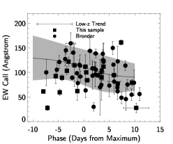
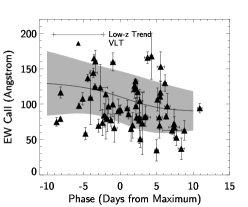
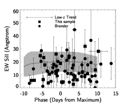
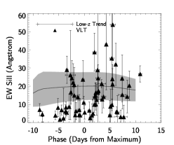
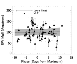
Figure 5: Each figure shows the low-z trend of the EW of either Ca ii H&K, Si ii or Mg ii as a solid black line with the $1\sigma$ region in grey. The high-z sample is shown as the points plotted over the top as squares and circles (Gemini) and triangles (VLT)

5 Results

5.1 Comparison between High-z Data and Low-z Trends

The high-z sample is divided into the Gemini sample (objects presented in this paper, plus those published in H05 and B08) and VLT samples in order to identify any systematic differences between the samples: none are seen in this analysis. Figure 5 shows the comparison for the three features in this analysis for both samples. The figures show the low-redshift trends seen in Figure 4 with the high-z points measured from the Gemini and VLT samples overplotted.

The high-z measurements for the Si ii feature appear to be smaller than the low-z trend. In order to look for systematic shifts, we make trends of the high-z data. The trends are calculated in a similar way to the low-z ones, except that the points are weighted according to the size of the error on the measurement, rather than applying a Gaussian weight based on phase. A rolling mean is applied with a bin-size of $\pm 3$ days. The mean for each phase bin is constrained so that there must be more than 10 equivalent width measurements within $\pm 3$ days in order for the value to stand. Consequentially, the trends are not evaluated at some early and later phases.

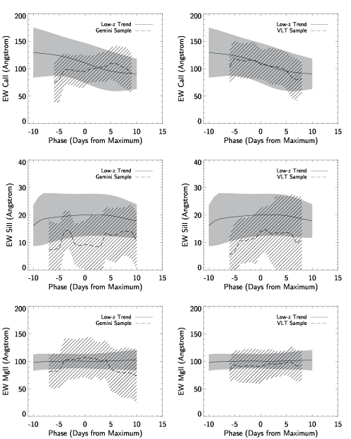
Figure 6: Each figure show the low-z trend of the EW of either Ca ii H&K, Si ii or Mg ii as a solid black line with the $1\sigma$ region in grey. The high-z trends are overplotted in blue (Gemini) and green (VLT) with the shaded region representing the $1\sigma$ RMS scatter

Figure 6 shows that for the Ca ii H&K and Mg ii features, the low- and high-z trends are approximately consistent. The Si ii feature shows a high-z trend which is consistently below the low-z one, as expected from the low-EW points seen in Figure 5. This will be discussed later. This is contrary to the observations of B08 which saw no difference between the high- and low-z populations in the Si ii feature. The difference between the high- and low-z populations that may have been observed for the Mg ii feature in B08 is not seen in this analysis which uses a larger high-z sample and a different method for generating low-z trends.

5.2 Correlations Between Spectroscopic and Photometric Properties

One of the reasons why there might be differences between the low- and high-z samples is because the spectral properties will be sensitive to the explosion physics of the supernovae. There is increasing evidence that there are two populations of supernova (e.g. Sullivan et al. (2006)) and that the prompt supernovae tend to be brighter and bluer. This will produce a drift in the mean photometric properties of SNe Ia as a function of redshift if the mix of prompt and delayed supernovae changes with redshift (Howell et al. 2007). $M_{B}$, the absolute B-band magnitude, is known to correlate with lightcurve width in the sense that more luminous SNe have higher stretch. We also know from B08 that EW Si ii is correlated with $M_{B}$, so brighter supernovae appear to contain less Si ii. These facts taken together imply that the mean spectral properties between the high- and low-z samples will be different in the sense that the high-z sample, where we expect a greater proportion of the prompt-type objects, should have a lower EW Si ii. This is indeed the effect seen in Figure 5. In the following we quantify the size of this effect and determine whether it explains the observed differences seen in Figure 5. First we quantify the correlations between spectral and photometric properties, stretch and colour, using a Spearman’s Rank correlation method.

We combine the Gemini and VLT samples into one high-z sample as the correlations are likely to be small effects. The high-z spectra in this study are also noisy and so there are large errors on the EW measurements. As the correlation coefficient calculation does not deweight objects based on the size of their error bars, we have grouped all the high-z objects together and ranked the objects according to the size of their error and used only the lowest 75% for this part of this analysis.The cuts for Ca ii H&K, Si ii and Mg ii correspond to error values of 18.1 Å, 9.7 Å and 19.3 Å respectively. The correlations are evaluated for all the high-z objects with errors less than the 75-percentile cut. The correlation coefficients are presented in Table 4.

Table 4: Correlation coefficients between the measured EWs and the light curve stretch and colour for the low-z, high-z and combined samples. The number of standard deviations from a null hypothesis is given in the final column.

Feature	Variable	Sample	$\rho$	$\sigma$ from null
Ca ii H&K	Stretch	Low-z	0.21	-0.66
		High-z	0.10	-1.0
		All	0.09	-0.91
	Colour	Low-z	0.44	-1.38
		High-z	0.12	-1.20
		All	0.21	-2.15
Si ii	Stretch	Low-z	-0.76	3.58
		High-z	-0.24	2.50
		All	-0.33	3.78
	Colour	Low-z	0.19	-0.89
		High-z	0.08	-0.80
		All	0.19	-2.12
Mg ii	Stretch	Low-z	-0.31	1.47
		High-z	0.09	-0.93
		All	0.03	-0.38
	Colour	Low-z	0.47	-2.22
		High-z	0.09	-0.85
		All	0.17	-1.87

The correlation analysis shows that the strongest correlations exist between stretch and EW Si ii, and this is seen in all samples at the 2.5–3.5$\sigma$ level. There are also weak correlations between the EW Si ii and colour for the combined sample, and for the low-z sample between EW Mg ii and colour. There also appears to be a slight correlation between the EW Ca ii H&K and colour. There appears to be no correlation between EW Ca ii H&K and stretch. We now examine the two most promising relations: EW Si ii and stretch; and EW Mg ii and colour.

5.2.1 EW Si ii and Stretch

The stretch-EW Si ii measurements are plotted in Figure 7 for the low-z (diamond) and high-z (square and triangle) points. Here the high-z Gemini and VLT samples are plotted separately in order to identify any possibly systematic offsets between the samples: none are seen. The best-fit was found using LINFITEX, part of MPFIT, which takes account of errors on both the variables. The low- and high-z relationships shown by the black lines are are:

$$s = (1.22\pm 0.03)+(-0.015\pm 0.002)\times EW_{SiII}\textnormal{\quad low-z}$$ (5)

$$s = (1.21\pm 0.01)+(-0.017\pm 0.001)\times EW_{SiII}\textnormal{\quad high-z}$$ (6)

The reduced $\chi^{2}$ for the fits are $\chi^{2}_{r}=2.2$ (low-z) and $\chi^{2}_{r}=2.7$ (high-z). The fits are consistent to within 1$\sigma$, although the errors on the gradient and intercept are correlated. We would expect the fits to be the same if the high- and low-z populations behave in the same way; however this does not mean that they must have the same distribution at high and low redshift.

It has already been established in B08 that there is a relationship between EW Si ii and $M_{B}$, the absolute magnitudes of the individual supernovae: the brighter the supernova, the smaller EW Si ii. This has been extended here to use lightcurve stretch instead of magnitude, as is shown in Figure 7, as $M_{B}$ is known to correlate with stretch. This relationship can potentially explain the difference seen between the low-z and high-z objects in Figures 5 and 6 above. Figure 8 shows that the stretch distribution is shifted to higher stretch for the higher redshift samples compared to the low-z one. The relationships seen in Figure 7 show that more higher stretch objects would mean more low-EW Si ii measurements.

Figure 7: Top: Stretch against EW Si ii for the low-z data. Bottom: Stretch against EW Si ii for the high-z Gemini (blue squares) and VLT (red triangles) data. In both plots, the black line represents the best-fit straight line to the data. The fits are given in Equations (5) and (6)

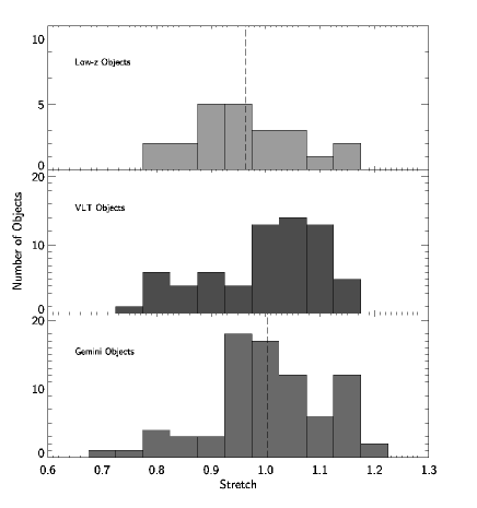
Figure 8: Histograms of the stretch distribution for the low-z (green), VLT (red) and Gemini (blue) samples. The dotted line marks the mean stretch for each sample. The low-z sample has a lower mean stretch than the two high-z samples.

To test whether the difference in mean stretch between the high- and low-z samples can be attributed as the cause of all the systematic shift in EW Si ii as seen in Figure 5, a predicted high-z mean EW was calculated based on the mean high-z stretch and the low-z relation from Equation (5). This predicted high-z mean EW Si ii can then be compared to the measured value.

From Figure 8, the mean stretches for the high- and low-z samples are $\overline{s}_{\textnormal{\footnotesize{low-z}}}=0.96$, $\overline{s}_{\textnormal{\footnotesize{Gem}}}=1.00$ and $\overline{s}_{\textnormal{\footnotesize{VLT}}}=1.00$, with standard deviations $\sigma_{\textnormal{\footnotesize{low-z}}}=0.10$, $\sigma_{\textnormal{\footnotesize{Gem}}}=0.11$ and $\sigma_{\textnormal{\footnotesize{VLT}}}=0.10$. Using the high-redshift standard deviation to produce upper and lower bounds and ignoring the errors on the fit in Equation (5), the predicted mean high-z EW Si ii values are 14.67 Å with a standard deviation of 7.34 Å (Gemini), and 14.67 Å with a standard deviation of 6.67 Å (VLT). Taking the weighted mean and standard deviations of the observed high-z trends in Figure 6 yields observed mean EW Si ii of 11.23 Å with a standard deviation of 4.58 Å (Gemini) and 11.05 with a standard deviation of 6.64 Å (VLT). Although the errors on the quantities are large, the predicted and observed high-z EW Si ii are in good agreement with each other.

Thus it appears that the difference in observed EW Si ii between the low- and high-z samples can be explained by the difference in the stretch distributions of the two samples, i.e. the differences are due to changing demographics rather than a new, unexplained form of evolution.

5.2.2 EW Mg ii and Colour

The relationships between colour and EW Mg ii in the low- and high-z data are plotted in Figure 9. Figure 9 highlights the differences in properties between the high- and low-z samples. The range of EW Mg ii values in the high-z data is much broader than for the low-z sample, but the reason is unclear. This could be because the low-z sample is too small to be representative of the SNe Ia population as a whole. The high-z sample is suffering from selection bias as a rough colour-cut is applied during high-z target selection and we do not see the range of supernova colours observed in the low-z sample.

Figure 9: Top: Colour against EW Mg ii for the low-z data. Bottom: Colour against EW Mg ii for the high-z Gemini (square) and VLT (triangle) data.

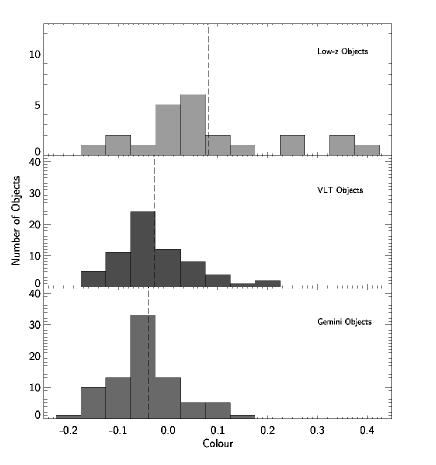
Figure 10: Histograms of the colour distribution for the low-z (green), VLT (red) and Gemini (blue) samples. The dotted line marks the mean stretch for each sample. The low-z sample has a redder mean than the two high-z samples.

Figure 10 shows that the colour distributions for all three samples are very different. The low-z sample contains a number of redder objects which aren’t seen in the high-z data. These are not underluminous, redder supernovae, but objects classed as core-normal.The Gemini distribution shows a strongly-peaked distribution around $c=0$ whereas the VLT distribution is more spread out. The mean colours for the samples are $\overline{c}_{\textnormal{\footnotesize{low-z}}}=+0.08$, $\overline{c}_{\textnormal{\footnotesize{Gemini}}}=-0.03$ and $\overline{c}_{\textnormal{\footnotesize{VLT}}}=-0.04$.

It is not possible to state anything conclusive about any relationship between colour and EW Mg ii as the data is very noisy at high-z and the sample at low-z is very small. This would be interesting to investigate further with better data as the relation could potentially reveal more about the supernova progenitor and be another test for an evolving population, but it is not possible at this time.

5.3 Applications of SNe Ia Spectra in Cosmological Studies

One of the aims of this study is to investigate potential uses for supernova spectra in the calibration of the objects for cosmological studies. This could be either as an alternative to the current method of photometric stretch and colour, or as a third calibrator, with the goal of reducing the scatter around the best-fit line on the Hubble diagram and hence improve the accuracy of cosmological parameter estimation. The large, spectroscopic dataset, with accompanying photometry lends itself well to this type of study.

5.3.1 Cosmology Fitter

In order to measure a scatter in the Hubble diagram, we must first fit the cosmology. In this section we detail the cosmological fitter used for this purpose. Throughout, we assume a flat universe with $w=-1$.

The supernova cosmology is fitted using a MINUIT-based, lighter-weight version of SIMPLE COSFITTER as opposed to a full Bayesian analysis used in Astier et al. (2006). We refit the data rather than using the cosmology found in Astier et al. (2006) because the samples used in the studies are different. A best-fit method is faster and sufficiently precise for this study.

SIMPLE COSFITTER takes the supernova apparent B-band magnitudes at maximum, $m_{B}$; the redshift, $z$; the supernova lightcurve stretch, $s$; and supernova lightcurve colour $c$ and performs a least-squared fit to find the best-fitting values of $\Omega_{M}$, $\alpha$, $\beta$ and $\mathcal{M}$ by minimising the $\chi^{2}$ where

$$\chi^{2} = \sum_{\textnormal{objects}}\frac{(\mu-5\log(d_{L}(z,\theta)/10\textnormal{\,pc}))^{2}}{\sigma^{2}(\mu)+\sigma^{2}_{int}}$$ (7)

and

$$\mu = m_{B}-\mathcal{M}+\alpha(s-1)-\beta c$$ (8)

$\theta$ stands for the cosmological parameters that define the fitted model, which in this case is simply $\Omega_{M}$; $\sigma(\mu)$ is the error on the observed distance modulus; and $\sigma_{int}$ is the intrinsic dispersion in the supernova absolute magnitudes (Astier et al. 2006). A good fit is obtained by varying the parameter $\sigma_{int}$ manually until the $\chi^{2}_{r}=1$; the other parameters are varied by COSFITTER itself. By assuming a value of $H_{0}$ then the mean supernova absolute magnitude $\overline{M_{B}}$ can be calculated from the fitted value of $\mathcal{M}$.

The code can be exploited to fit alternatives to stretch and colour, e.g. equivalent width. It was also adapted to fit for a fourth variable which has a linear contribution to the distance modulus. For instance, the fit could be performed using equivalent width as a third possible calibrator:

$$\mu = m_{B}-\mathcal{M}+\alpha(s-1)-\beta c+\gamma EW$$ (9)

The code also enables evaluation of $\mathcal{M}$, $\alpha$, $\beta$ and $\gamma$ within a fixed cosmology.

5.3.2 Cosmological Parameters Derived From Photometric Data

In this section, we fit the cosmology to the data sample in order to have a baseline to compare against when testing for spectroscopic calibrators.

As stated in Section 4.2, the low-z sample used for the spectroscopy study is not sufficient for cosmology-fitting. This is because most of the objects are not in the Hubble flow and their peculiar velocities affect their redshifts and hence their distances are very poorly constrained. To account for this, we use the low-z sample from Astier et al. (2006) with photometry fitted using SiFTO, but removing the objects marked with $\ast$ in Table 3, to keep the cosmology and spectroscopy samples entirely separate. We also make stretch and colour cuts on the sample to remove any possible outliers which may not be fully described by the width-brightness or colour relations. The cuts are $0.75\leq s\leq 1.25$ and $-0.25\leq c\leq 0.25$ which leaves a sample of 32 low-z objects, 75 Gemini objects and 66 VLT objects. This is similar to the cuts that would be applied for a full cosmology analysis.

For the first fit no stretch or colour correction was applied to the data. This is designated Fit A in Table 5. The fit shows that the intrinsic dispersion ($\sigma_{int}$) must be set to be quite high (0.255 mag) in order to obtain a $\chi^{2}_{r}\approx 1$. The value of $\Omega_{M}=0.462$ is higher than current measurements which employ stretch and colour correction (e.g. Astier et al. (2006)), but this is to be expected because at higher redshift the supernovae tend to be brighter and bluer which causes the fit to favour a higher matter fraction.

In Fit B, stretch and colour corrections are applied and the resulting best-fit value of $\Omega_{M}$ is much lower. The value is within 2 standard deviations of that published in Astier et al. (2006). The latest full analysis of SNLS data finds, $\Omega_{M}=0.268\pm 0.020$ (Sullivan et al. (in prep.)), and so the value calculated in Fit B is within 3 standard deviations. The value of $\alpha$ is very similar to the one achieved from the full analysis, and $\beta$ is very different from the value published in Astier et al. (2006), but in close agreement with the latest value from the SNLS analysis ($\beta=2.9$). This is due to the fact that the treatment of the $\beta$ parameter in the fitting methods has changed since Astier et al. (2006). Fit B shows a reduced RMS compared to Fit A which shows that the calibration applied using stretch and colour corrections are important. Applying these corrections also reduces the intrinsic scatter required for a good fit. It is a result similar to this which is the goal of this part of the study.

Table 5: Cosmology fits table. The fit from Astier et al. (2006) is included for reference. Fits C, D and E were made without the low-z sample and fixing the cosmology to the values from Fit B. Fit F was made without the use of the low-z sample, but the cosmology was not fixed. Parameters which were fixed are marked with a *. The quoted values of $\sigma_{int}$ are those used to obtain the best fits.

Fit

Extra Calibrator

$\sigma_{int}$

RMS

$\Omega_{M}$

$\alpha$

$\beta$

$\gamma$

$\mathcal{M}$

(mag)

(mag)

(mag)

Astier

–

–

–

0.263$\pm$

0.053

1.52$\pm$

0.14

1.57$\pm$

0.15

–

23.85$\pm$

0.03

A

–

0.255

0.260

0.462$\pm$

0.065

–

–

–

24.091$\pm$

0.045

B

–

0.12

0.181

0.197$\pm$

0.031

1.28$\pm$

0.14

3.21$\pm$

0.19

–

23.999$\pm$

0.025

C

Ca ii H&K

0.10

0.176

0.197*

1.28*

3.21*

0.001$\pm$

0.001

24.050$\pm$

0.028

D

Si ii

0.10

0.183

0.197*

1.28*

3.21*

0.006$\pm$

0.002

24.084$\pm$

0.030

E

Mg ii

0.10

0.177

0.197*

1.28*

3.21*

0.000$\pm$

0.001

24.044$\pm$

0.039

F

Si ii

0.10

0.193

0.214$\pm$

0.053

1.50$\pm$

0.18

3.49$\pm$

0.24

0.007$\pm$

0.002

24.123$\pm$

0.054

Figure 11: Hubble diagram for Fit B (solid line) which uses stretch and colour corrections, compared to the cosmology fit from Astier et al. (2006, dashed). The data used are the low-z cosmology sample from Astier et al. (2006), and all the VLT and Gemini objects from the samples defined in Section 2. Stretch and colour cuts are applied. In both plots, the black points are calculated using the distance moduli from the apparent magnitude of the supernova fitted by SiFTO and the cosmological parameters from Fit B, correcting for stretch and colour. The lines represent the distance moduli calculated from Equation (8). The bottom plot shows the residuals from Fit B (see Section 5.3.3 for definition) compared to the Astier cosmology.

5.3.3 Hubble Residual Correlations

Now the cosmology has been fitted to the data, residuals from the fit can be plotted against spectral features and possible alternative calibrators found. The Hubble residuals, $R$, as shown in Figure 11, are defined as

$$R = m_{B}-m_{\textnormal{\footnotesize{cosmo}}}(z,\Omega_{M})$$ (10)

where $m_{B}$ is the observed B-band apparent peak magnitude and $m_{\textnormal{\footnotesize{cosmo}}}$ is derived from the cosmological parameters. The assumed cosmology is that measured using Fit A i.e. $\Omega_{M}=0.462$ in a flat universe. The correlations with the photometric quantities stretch and colour are also presented as a guide as, naturally, strong correlations are expected for these variables. As in Section 5.2, we use only the high-z EW measurements from the least noisy 75% of the sample.

For the low-z sample, the method of calculating the observed distance modulus is slightly different as not all the objects are in the Hubble flow. For five very nearby objects (see Table 16) which are not in the Hubble flow we use distance moduli measured from their host galaxies either using Cepheid variable stars (Saha et al. 2006) or galaxy surface brightness fluctuations (Ajhar et al. 2001). These values minus the value of $\overline{M_{B}}$ determined from the best-fit value of $\mathcal{M}$ from Fit A and assuming $H_{0}=70$kms^-1Mpc^-1, are used as $m_{\textnormal{\footnotesize{cosmo}}}$. For 5 other objects, they are situated in host galaxies with $z\geq 0.02$ and can be assumed to be in the Hubble flow and so the same method as the high-z sample to calculate $m_{\textnormal{\footnotesize{cosmo}}}$ is used. Plots of the low-z and high-z data are shown in Figure 12. The correlations are calculated and tabulated in the same way as Table 4 and presented in Table 6.

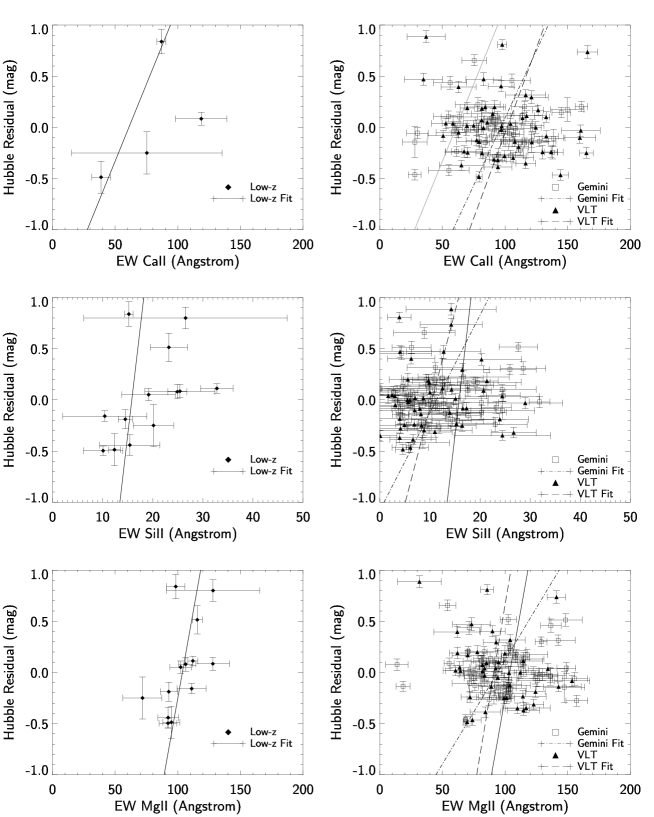
Figure 12: Hubble Residual - EW Plots for the low-z (left column) and the high-z (right column) objects. The best-fits to the lines are also shown. Solid line – low-z; dot-dashed – Gemini; dashed – VLT.

Table 6: Correlations between photometric and spectral properties and the Hubble residuals. There are not enough low-z objects with EW Ca ii H&K measurements to measure a correlation.

Variable	Sample	$\rho$	$\sigma$ from null
Stretch	Low-z	-0.45	1.62
	Gemini	-0.45	4.04
	VLT	-0.51	4.10
Colour	Low-z	0.79	-2.73
	Gemini	0.51	-4.48
	VLT	0.58	-4.67
EW Ca ii H&K	Low-z	–	–
	Gemini	0.09	-0.60
	VLT	-0.13	0.97
EW Si ii	Low-z	0.72	-2.59
	Gemini	0.13	-0.94
	VLT	0.10	-0.71
EW Mg ii	Low-z	0.78	-2.80
	Gemini	0.05	-0.38
	VLT	-0.29	1.87

The strong correlations between stretch and colour and Hubble residual in Table 6 show that the current low- and high-z spectral features should not be used as direct replacements for either of the photometric properties as the relations are much weaker. The strongest correlation between one of the high-z spectral features and the residuals is for EW Mg ii for the VLT sample, but this is not seen in the Gemini data - the correlation goes in the opposite direction. However, the linear fits to the data in Figure 12 where points are weighted according to their errors show the best-fit lines all have positive gradients, implying that the negative correlation coefficient seen in the VLT data is spurious. By comparing Table 6 and Figure 12, we can see that even applying a cut to remove the most noisy points from the high-z data, the correlation coefficient does not necessarily represent the best way to look for a relation between two quantities as it is affected by outliers.

Instead of looking to replace stretch or colour with one of the EW measurements, it might be more instructive to look for a correlation which exists between the EW and the Hubble residual after the application of stretch and colour correction. To do this, we fix the cosmology and values of $\alpha$ and $\beta$ to $\Omega_{M}=0.197$, $\alpha=1.28$ and $\beta=3.21$ as in Fit B, and use the adapted version of COSFITTER to fit Equation (9).

To see just how great an improvement can be made, the instrinsic dispersion was allowed to vary and Equation (9) fitted allowing $\mathcal{M}$, $\sigma_{int}$ and $\gamma$ as the free parameters. The cosmology must be fixed as the objects in the low-z cosmology sample do not have accompanying spectra and so could not be used to anchor the Hubble diagram for these fits. The results of this process are given by Fits C, D and E in Table 5.

The results in Table 5 show that by adding in a third calibrator, the intrinsic dispersion necessary for a good fit can be decreased, as expected. The Ca ii H&K and Mg ii features show values of $\gamma$ consistent with 0 and so they are ruled out as possible calibrators. However, for the Si ii feature $\gamma$ is three standard deviations from zero and produces a value of $\mathcal{M}$ consistent with the one in Fit B. The RMS is comparable to the one obtained in Fit B as well.

In order to test whether this result is meaningful, the constraints on $\alpha$, $\beta$ and $\Omega_{M}$ were relaxed so they were free parameters. Even without a low-z sample to anchor the Hubble diagram at low redshift, the fit using EW Si ii as a third calibrator still gave reasonable values for the parameters, denoted as Fit F in Table 5. However, the RMS scatter was increased slightly to 0.193 mag.

From this is is clear that Si ii could have a role to play in SNe Ia calibration for cosmology. However, with the large errors on the high-z EW measurements, the RMS scatter around the best-fit cosmology do not improve and it is not possible to draw any firm conclusions as to the value of $\gamma$. Instead, in Section 5.4, we demonstrate that the relationship between EW Si ii and stretch in the low-z sample can be exploited to reduce the residuals on the Hubble diagram by reducing the scatter on $M_{B}$ measurements.

5.4 EW Si ii as a Cosmological Calibrator

Drawing on the fact that we have seen that EW Si ii and photometric stretch are correlated, and that there is a strong correlation between the Hubble residuals and the low-z EW Si ii, we will explore the possible use of EW Si ii as a calibrator for the cosmology in place of stretch for the low-z sample. Here the errors on the EW are smaller so it is possible to be more definite about the potential of the calibrator.

Figure 13: The two sub-samples of the low-z data are shown. Those with closed circles do not have known distance moduli and are used to define the spectral-stretch relations (black line). Those with open circles will be used to test the relation and are not included in the fit.

We divide the objects in the low-z spectroscopy sample which have photometry into two independent sub-sets in order to have a sample to define the relation and a separate one to test its use. The first sample (i) contains the objects with no reliable absolute distance measures, i.e. those without Cepheid or surface brightness fluctuation distances and not in the Hubble flow (those marked with a ^† only in Table 3); and the second sample (ii) containing the rest (those marked as ^†‡). The two samples are illustrated in Figure 13 as open circles for the objects with distance measurements and closed circles for those objects without. Using sample (i), the relation between stretch and EW Si ii is refitted to derive an expression for “spectral stretch”, $s_{\textnormal{\footnotesize{spec}}}$, using LINFITEX. The best-fit is given by

$$s_{\textnormal{\footnotesize{spec}}} = (-0.021\pm 0.005)EW_{\textnormal{\footnotesize{SiII}}}+(1.29\pm 0.07)$$ (11)

where $\chi^{2}_{r}=1.55$. This fit is different from the ones in Equations (5) and (6) as fewer objects are used. The remaining 10 low-z objects were corrected for stretch and also spectral stretch according to the relation

$$M_{B} = m_{B}-\mu+\alpha(s-1)$$

where $s$ can either be the normal photometric stretch or spectral stretch as fitted in Equation (11). We then plot $M_{B}$ against $\mu$ for illustration purposes, and measure the weighted-mean, $\overline{M_{B}}$, and the RMS scatter about the mean. This is shown in Figure 14. The values of $\overline{M_{B}}$ and the RMS are shown on each plot and summarised in Table 7. For the purposes of this exercise we take the values of $\Omega_{M}$ and $\alpha$ from Fit B. The right-hand column of Figure 14 shows the effect of also adding a correction for supernova colour.

Figure 14: Comparing spectral stretch correction to photometric stretch correction with and without colour correction. The value of $\overline{M_{B}}$ given on the plot is the weighted mean of the points after the stretch correction. Without colour correction (left column) the RMS before any stretch correction is 0.45 mag and the mean absolute magnitude $\overline{M_{B}}=-18.94$. With colour correction but no stretch correction (right column), $\overline{M_{B}}=-19.19$ mag and the RMS is 0.24 mag

Table 7: A summary of the vaules of $\overline{M_{B}}$ and the RMS scatter about the mean for the fits in Figure 14.

Corrections Applied	$\overline{M_{B}}$	RMS
	(mag)	(mag)
None	-18.94	0.45
Spectral stretch	-19.11	0.38
Photometric stretch	-19.00	0.44
Colour	-19.19	0.24
Colour + Spectral stretch	-19.29	0.33
Colour + Photometric stretch	-19.25	0.20

Table 7 shows that the lowest RMS is obtained when using photometric stretch and colour together, but when no colour correction is made, spectral stretch correction produces a lower RMS than photometric stretch.

It is not possible to apply this correction to the high-z supernovae and see any improvement in the data due to the large errors on EW Si ii, but in the future with a sample of well-measured equivalent widths it is possible that spectral stretch could replace photometric stretch. This would mean that once the supernova was identified fewer photometry points would be needed to fit the light curve, only the B-band magnitude at maximum and the redshift would be needed: supernova colour could be measured from synthetic photometry of a spectrum obtained around maximum light. However, the stretch-EW Si ii relation needs better calibration first using, for example, a large sample of low-z supernovae either with known host galaxy distances or within the Hubble flow. As seen from the $\gamma$ parameter analysis in the noisy high-z data, as shown in Table 5, if corrections for photometric stretch, colour and spectral stretch/EW Si ii can all be combined then there is the potential that calibration could be improved.

6 Discussion

6.1 Tests for Evolution

The comparison between the high-z and low-z trends seen in Figure 6 shows that for the Ca ii H&K and Mg ii features, the high-z sample is consistent with the low-z trends, but the scatter on the data is quite large. For the Si ii feature, a large number of low equivalent width measurements are seen in the high-z data and the high-z trend is consistently below the low-z one. This can be explained as a change in the demographics. In Section 5.2.1 we see that light curve stretch is correlated with EW Si ii. At higher redshift, due to the “A+B” model we expect more of the prompt component which are brighter and bluer as more ⁵⁶Ni is thought to be produced during the explosion. This would produce less IME which is reflected in the lower EW Si ii.

To the level of current precision, the variation in mean EW Si ii between high and low redshift can be understood in terms of the combination of a change of demographics within a two-component SN model and an observed correlation between photometric stretch and EW Si ii. Therefore, we see no evidence for an additional bias that is not already accounted for by the standard photometric stretch and colour corrections. However, in future experiments which may go to even higher redshift to look for $w=w(z)$ (models where dark energy is not a cosmological constant) will need a higher level of precision. Future cosmological studies observing to $z=1.7$ will need a precision of 2% in the standardisation of supernova magnitudes if they are to keep systematic errors smaller than statistical errors, and it not yet clear whether the current methods of calibration will be suitable for this (Howell et al. 2007). We also know that the width-brightness relation may not be valid for supernovae with large stretch such as SN 2001ay-like objects.

It will only be possible to make a strong statement regarding the evolution of SNe Ia when there is a large, unbiased sample of low-z spectra. In Figure 8 we have only 3 low-z objects in the $s=1$ bin, compared to 14 in the VLT sample and 17 in the Gemini sample. Future surveys such as Palomar Transient Factory (Law et al. 2009) and SkyMapper (Keller et al. 2007) will largely address this problem.

6.2 Implications for Cosmology

The origin of the width-luminosity relation is well-understood to first order: a variation in the amount of ⁵⁶Ni alters the amount of gamma-rays emitted due to radioactive decay to ⁵⁶Co and ⁵⁶Fe which are absorbed and thermally reemitted by the expanding ejecta (Colgate & McKee 1969; Arnett 1979). The more ⁵⁶Ni produced, the wider the light curve (Arnett 1982). This also means the production of less IME, which is reflected in Figure 7 (see also Figure 2 in Sullivan et al. 2009). What causes the varying amount of ⁵⁶Ni is not understood although it may be due in part to the way that burning of carbon and oxygen occurs in the supernova, or the metallicity of the progenitor. The relation between stretch and EW Si ii from Figure 7 is exploited in Section 5.4 for the low-z dataset to reduce the scatter of the objects on the Hubble plot by correcting $\overline{M_{B}}$ using spectral stretch.

The origins of supernova colour are more complex than stretch and not as well-understood. At high redshift, colours may be affected by the environment surrounding the supernova simply due to the fact that it is not possible to separate the supernova light from the surrounding interstellar and circumstellar medium (see Conley et al. 2007, for a discussion of the effect of dust and the colour parameter on cosmology). In addition those effects, from studies in the local universe, there is known to be an intrinsic difference in supernova colours as well (Phillips 1993). In Table 6 we see that supernova colour has a stronger correlation with Hubble residual than stretch, implying that it is more important for calibration purposes.

Another application for spectral stretch is that it may allow more supernovae to be added to the low-z sample for cosmology. Currently, most SNe Ia have either good photometric coverage or good spectroscopic coverage, but not both. For instance, in the spectroscopic sample used for this study, only 5 objects overlap with the Astier et al. (2006) cosmology sample. By taking the objects that have good spectroscopic coverage, instead of using photometrically-derived properties to calibrate them, spectral stretch could be used. This would also require a B-band magnitude at maximum, or interpolated from other data, and a known distance modulus or redshift. There is not yet a spectral replacement for colour, but the EW Mg ii-colour relation seen in the low-z sample could be exploited for this purpose when the relationship is better quantified.

For future studies out to $z=1.7$, Howell et al. (2007) have shown that supernova calibration needs to be better than 2% in magnitude in order to keep systematic errors below the level of statistical errors. By introducing a third calibrator based on EW Si ii into the cosmology in Section 5.3.3 we find a non-zero value for the constant $\gamma$ whilst achieving a similar RMS scatter around the best-fit cosmology as when using standard photometric stretch and colour corrections. The estimate of $\Omega_{M}$ is also closer to the current value from the full Bayesian analysis of SNLS data. In the future with higher signal-to-noise spectra, the EW Si ii may provide a further method of cosmological calibration. At the moment, the best fit is not approaching the 2% level. This can be done with more observations with high signal-to-noise spectra and good photometric follow-up of discoveries.

6.3 Improvements

6.3.1 Galaxy Subtraction Method

The methods presented in Section 3.3 detail the way host galaxy contamination is removed from the spectra. This is made somewhat more difficult for the Gemini objects which were not observed at parallactic angle and hence the spectra suffer from slit-losses. The objects from the VLT sample were observed using an ADC and so this is less of a problem. Extraction of spectra from the host galaxy and the supernovae separately was not usually possible due to the small angular size of the galaxy on the sky. In order to subtract off host galaxy light, we must make an assumption about the nature of the background light, and we assume that it is a flat background in the slit. This assumption is reasonable in most cases, but it can fail when the supernovae are situated in the very centre of the host, or on the outskirts.

Another limitation is the number of galaxy template spectra available for the subtraction. In order to make a better subtraction, ideally we would reobserve the host galaxies after the supernova light has faded with an identical set-up. However, there will be slight variations in the seeing and airmass so the correction would still not be perfect. Another method would be to use the CFHT imaging directly to aid subtraction. Photometry-Assisted Spectral Extraction (PHASE; Baumont et al. 2008) has been developed and used on SNLS-VLT spectra to extract the supernova spectrum with an extraction window determined from the position of the target in the imaging data (Balland et al. 2009). A $\chi^{2}$-minimisation is used to evaluate the contribution of galaxy and supernova in each pixel to produce a spectrum composed of only supernova light. This method produces clean spectra for approximately 70% of observations, but when the supernova is close to the centre of the host, or the fractional contamination of the the spectrum is high, the method cannot separate the two components. These are two of the occasions when the multicolour host galaxy subtraction method also fails so PHASE could be used as an alternative to the method used in this study, but not as a replacement.

6.3.2 Low-z Trends

In comparison to the large number of high-z objects included in this analysis, there are only 14 objects used to make the low-z trends for the Ca ii H&K feature, and 25 for the Si ii and Mg ii features. The sample is biased towards supernovae in bright, elliptical hosts which will tend to host redder supernovae with lower stretch (the delayed component from the two-component model). This can be seen in Figure 8. The sample is also drawn from many sources where the photometric coverage is different. To do a study of this kind in the future to an increased level of precision we would require a large homogeneous sample of low-z spectra and photometry.

The trends shown in Figure 4 reflect the diversity seen in the low-z objects, an advantage of using the EW measurements directly; however, there is a much larger scatter on the high-z data. Some of this scatter will be due to a lower signal-to-noise ratio in the high-z data, but some might be intrinsic to the supernova populations that we do not observe in the low-z sample due to its limited size. The lack of a well-calibrated set of supernova spectra which cover the blue Ca ii H&K feature limits this part of the study particularly. There might be additional subtypes in the supernovae population, or transitional objects, which have not yet been identified. It is not yet clear whether there is a continual class of objects from underluminous SN 1991bg-like supernovae (Filippenko et al. 1992) to overluminous SN 1991T-like objects (Filippenko et al. 1992), or whether the progenitors are different (for example Benetti et al. 2005; Branch et al. 2006). Indeed, unusual objects objects falling outside these classes are now observed.

One of the most interesting results to come out of the low-z trend of the Mg ii feature is the fact that this feature seems to be constant with time and with very little scatter between objects. The feature is not made up of solely Mg ii, but also contains Fe ii and Fe iii which are thought to be sensitive to temperature variations in the supernova and drive the relation between $\mathcal{R}_{642/443}$ and colour described in Bailey et al. (2009). Furthermore the recombination from Fe iii to Fe ii changes the opacity of the ejecta and causes the secondary maximum in the supernova lightcurves (Kasen 2006). We see weak correlations between EW Mg ii and colour in Figure 9, but there is a large variation in the relations between the low- and high-z data. As there is a larger range of colours observed in the low-z sample compared to the high-z sample, we would expect the any diversity to be seen in the low-z trend. A larger data-set at low-z would enable this to be investigated further.

7 Conclusions

The aims of this study were to observe spectroscopically potential Type Ia supernovae and confirm their type and redshift in order for them to be used for cosmology; to study the spectra of the objects themselves to verify their use as cosmological standard candles; and to investigate new ways the spectral information can be used to calibrate the objects for cosmology.

The first aim is easily satisfied. Here we present observations of 95 targets, 68 of which were confirmed as SNe Ia or probable SNe Ia events. 8 events were confirmed as being core-collapse in nature, leaving 19 observations as probably not Ia in nature or of unknown type. The spectra are presented in Appendix B. The spectroscopic observations of such a large dataset, especially when combined with other SNLS observations, provide an opportunity to study supernovae covering billions of years of cosmic look-back time. SNLS provides not only spectroscopic coverage, but complete light curves in four bands to fit the photometric properties such as apparent magnitude, stretch and colour; and deep images of the host galaxy in five bands. In total, spectral analysis was possible for 144 objects drawn from SNLS survey work at the Gemini and VLT telescopes, covering a redshift range of $0.184\leq z\leq 1.002$.

The second aim was investigated in Section 5.1 where high-z equivalent width measurements of the Ca ii H&K, Si ii and Mg ii spectral features are compared to trends seen in a low-z sample. We find that for the Ca ii H&K feature, the scatter on the measurements at low- and high-z is large, but the features appear to be consistent with each other. The Mg ii feature has a much lower scatter at low redshift than with high-z measurements and the statistical comparison between the two sample yields $\chi^{2}_{r}>1$; however, there does not appear to be a systematic shift in the mean value of EW Mg ii between the two samples. The Si ii feature has a lower trend at high redshift compared to low redshift. This is explained by the fact that EW Si ii is seen to be anticorrelated with photometric stretch. At high redshift we see more of the prompt component from the “A+B” model which are brighter and have a broader light curve due to greater ⁵⁶Ni production. These supernovae have larger stretches and hence smaller EW Si ii. We also observe different correlations between EW Mg ii and photometric colour for the low-z and high-z samples. This difference is probably due to a difference in sample selection and the colour-cut introduced in the high-z target selection in particular. The origin of any possible relationship between colour and EW Mg ii is not understood, but may be connected to the balance between Fe ii/Fe iii which are also present in the feature. It does not appear to systematically affect the comparison of EW trends despite the high-z sample being bluer than the low-z sample. We find nothing within the dataset to introduce doubt as to the use of SNe Ia as standardisable candles for cosmology.

The final aim, to exploit spectral properties to aid cosmological calibration is studied in Section 5.3. We find that the spectral features do not correlate with Hubble diagram residuals as strongly as photometric stretch or colour, but significant relationships are seen between the residuals and EW Si ii and EW Mg ii. This is to be expected as we see relations between EW Si ii and EW Mg ii, and stretch and colour, respectively. The high-z data are too noisy to be used to produce a spectroscopically-calibrated Hubble diagram. However, we demonstrate that such a calibration may be possible by defining a spectral stretch from a sub-set of the low-z sample based on the observed relationship between EW Si ii and photometric stretch. This is then applied to other low-z supernovae with known distance moduli or which are within the Hubble flow and we demonstrate that this reduces the scatter on the measurement of the absolute magnitude. The spectral stretch correction reduces the RMS on the measurement of $\overline{M_{B}}$ to comparable, in fact slightly smaller value than that obtained by photometric stretch correction, although this is demonstrated for a small sample of objects.

Appendix A Data Tables

Table 8: Table of observations. ¹ Measured using GEMSEEING, ² Measured using IMEXAM, ³ R150 observation, ⁴ Second night of data only used ⁵ First night of data only used

SN	RA	Dec	UT Date	Exposure Time	Mode	$\lambda_{cent}$	Seeing
(SNLS name)	(J2000)	(J2000)		(s)		(nm)	(′′)
05D4bo	22:16:44.630	-17:20:12.37	2005-07-14	2700	N&S	720	0.43
06D1bt	02:24:59:57	-04:01:05.43	2006-08-31	5400	N&S	720	0.45
06D1bz	02:25:07.62	-04:42:06.58	2006-08-22	5400	N&S	720	0.52
06D1ck	02:26:25.37	-04:40:43.80	2006-08-31	3600	N&S	720	0.40
			2006-09-01	1800	N&S	720	1.03
06D1dt	02:27:15.20	-04:35:44.88	2006-09-23	3600	C	680	0.51
06D1gg	02:26:28.56	-04:44:54.29	2006-09-23	2400	C	680	0.66
06D1gu	02:24:33.91	-04:17:37.80	2006-11-18	5400	N&S	720	0.37
06D1hl	02:26:42.95	-04:18:22.34	2006-12-11	5400	N&S	720	0.36
06D1jp	02:25:48.07	-04:17:56.02	2006-12-22	7200	N&S	720	0.61
06D2iz	10:00:34.76	02:19:20.17	2006-12-21	5400	N&S	720	0.64
06D2ja	10:00:33.51	02:28:01.01	2006-12-21	3600	N&S	720	0.46
06D2ji	09:59:51.03	01:51:50.14	2006-12-19	7200	N&S	720	0.66
			2006-12-20	1800	N&S	720	0.38
06D2js	10:02:15.70	02:35:06.62	2006-12-25	7200	N&S	720	1.10
06D2ju	10:01:34.65	02:26:42.72	2006-12-24	5400	N&S	720	0.83
06D3ed	14:18:47.82	52:45:23:28	2006-05-27	2400	N&S	720	0.82
06D3el	14:17:01.06	52:13:56.84	2006-05-27	5400	C	680	0.72
06D3et	14:22:04.76	52:20:18.30	2006-05-31	5400	N&S	720	0.56
06D3fp	14:20:18.62	52:53:49.62	2006-06-18	2600	C	680	0.55
06D3fr	14:19:20.24	52:31:50.11	2006-06-29	3600	C	680	1.07
06D3fv	14:21:03.31	53:00:52.77	2006-06-25	1800	N&S	720	0.73
			2006-06-29	5400	N&S	720	0.65
06D3gg	14:20:17.36	53:10:42.27	2007-07-20	3600	N&S	720	0.51
06D3gh	14:18:31.38	52:26:34.69	2006-06-30	5400	N&S	720	0.41
06D3gn	14:17:44.61	52:21:40:42	2006-07-06	2700	C	680	0.40
06D3gx	14:17:03.36	52:56:21.82	2007-07-27	3600	N&S	720	0.52
06D3hd	14:20:42.76	52:14:20.27	2006-07-18	3600	C	680	0.72
06D4dh	22:14:19.70	-17:35:06:23	2006-07-30	5400	C	680	0.51
06D4dr	22:16:46.00	-17:20:45.49	2006-08-19	4800	N&S	720	0.44
06D4fc	22:13:52.30	-17:19:30.31	2006-09-23	5400	N&S	720	0.39
06D4fy	22:14:06.22	-17:34:19.34	2006-09-16	5400	N&S	720	0.39
06D4gn	22:15:14.81	-17:23:01.36	2006-09-22	7200	N&S	720	0.42
06D4hc	22:15:40.52	-18:09:08.71	2006-10-13	5400	N&S	720	0.96
07D1cx	02:24:58.48	-04:01:54.23	2007-11-10	3600	N&S	720	0.44
				3600		715
07D1ds	02:25:24.44	-04:18:49.29	2007-11-10	3600	N&S	720	0.41
				3600		720
07D1dv	02:26:51.27	-04:47:18.29	2007-11-10	1800	N&S	720	1.06
			2007-11-11	1800			0.51
				3600		715
07D1ea	02:25:14:77	-04:55:39.80	2007-11-13	3600	N&S	720	0.45
				3600		715
07D2bu	09:59:27.590	02:33:03.48	2007-03-15	5400	N&S	720	0.93
			2007-03-16	1800			0.63
			2007-03-17	3600			0.77
07D2cy	10:01:49.486	02:40:59.09	2007-03-22	3600	N&S	720	0.82
			2007-03-22	5400		715	0.51
07D2kc	10:01:07.19	02:02:28.65	2007-12-20	900	C	680	0.67
				1800		675
07D2ke	10:01:04.73	01:59:31.81	2007-12-20	900	C	680	0.80
				900		675
07D2kh	10:00:28.94	02:13:39.65	2008-01-04	3600	N&S	720	0.63
				1800		715
			2008-01-06	1800			0.32
07D2ki	10:00:26.69	01:56:48.87	2008-01-05	3600	N&S	720	0.54
				1800		715
			2008-01-08	3600			0.54
07D2kl	09:59:16.95	02:31:28.13	2008-01-4	3600	N&S	720	0.48
				3600		715

Table 9: continued

07D3ae	14:17:33.70	52:31:27.17	2007-01-25	2400	C	680	0.57
07D3af	14:19:05.01	53:06:08.98	2007-01-27	2400	C	680	1.12
07D3ai	14:19:06.711	52:40:11.69	2007-02-14	3600	C	680	0.49
07D3am	14:22:36.55	52:20:26.26	2007-01-23	3600	C	680	0.70
07D3ap	14:18:10.26	52:23:07.38	2007-01-23	3600	N&S	720	0.54
07D3bb	14:18:10.31	52:18:26.38	2007-01-25	7200	N&S	720	0.46
07D3bo	14:20:58.408	52:20:37.22	2007-02-14	5400	N&S	720	0.54
			2007-02-15	1800
07D3bp	14:21:01.32	52:13:37.19	2007-01-27	7200	B&S	720	0.75
07D3bt	14:21:25.719	52:58:13.67	2007-02-22	9000	N&S	720	0.55
07D3cn	14:16:17.255	52:32:22.60	2007-03-24	3600	N&S	720	0.50
			2007-03-25	5400		715	0.41
07D3cr	14:18:12.821	52:19:04.57	2007-03-20	7200	N&S	720	0.41
07D3cu	14:20:56.531	52:15:13.36	2007-03-24	2400	C	680	0.49
				2400		675
07D3da	14:20:06.236	52:16:16.64	2007-03-21	3600	N&S	720	0.36
				3600		715
07D3dj	14:22:40.795	53:02:14.69	2007-04-12	3600	C	680	0.44
07D3do	14:20:35.683	52:44:48.58	2007-04-10	3600	N&S	720	0.54
				3600		715
07D3ea	14:21:16.116	52:40:07.88	2007-04-12	3600	C	680	0.47
			2007-04-14	1200			0.66
07D3ey	14: 19:18.944	53:04:35.92	2007-05-14	3600	N&S	720	0.47
				3600		710
07D3fi	14:21:24.800	53:10:40.10	2007-04-23	3600	N&S	720	0.77
				3600		710
07D3gm	14:18:32.321	52:43:29.62	2007-05-19	3600	N&S	720	0.47
				3600		710
07D3hl	14:16:25.147	53:08:33.66	2007-06-09	3600	N&S	720	0.72
				3600		715
07D3hu	14:21:14.560	52:47:53.41	2007-06-11	3600	N&S	720	0.37
				1800		715
07D3hv	14:21:05.942	52:53:36.62	2007-06-11	3600	C	680	0.43
07D3hw	14:21:48.410	52:30:33.64	2007-06-08	3600	N&S	720	0.53
				3600		715
07D3hz	14:20:29.569	52:23:56.79	2007-06-10	3600	C	680	0.54
07D3ib	14:17:10.791	53:04:46.91	2007-06-16	3600	N&S	720	0.74
				1800		715
			2007-06-18	1800			0.89
07D3it	14:18:08.730	52:25:04.06	2007-07-16	3600	N&S	720	0.50
				3600		715
07D4fl	22:16:13.16	-18:11:46.00	2007-11-13	1800	N&S	720	0.47
				3600		715
08D1aa	02:27:37.13	-04:03:02.64	2008-01-27	1800	N&S	720	0.69
				1800		715
			2008-02-13	1800		720	0.98
08D2aa	10:01:52.77	02:15:57.74	2008-01-15	1800	N&S	720	0.76
			2008-01-17	1800			0.95
				1800		715
08D2ad	10:00:59.19	01:45:27.31	2008-01-09	1800	N&S	720	0.60
			2008-01-10	3600
08D2au	10:02:01.84	02:15:03.76	2008-01-17	1800	N&S	720	0.60
				1800		715
08D2bj	09:58:51.48	02:07:07.38	2008-01-10	3600	N&S	720	0.42
				3600		715	0.47
			2008-01-12	1800		715
08D2ch	10:01:39.61	02:06:57.56	2008-02-12	1800	N&S	720	0.68
				1800		715
08D2cl	09:59:28.55	02:29:49.02	2008-02-12	3600	N&S	720	0.94
				1800		715
08D2dr	10:01:54.13	02:04:01.96	2008-02-28	1200	C	680	0.66
				1200		675
08D2dz	09:58:53.07	01:44:19.21	2008-03-05	3600	N&S	720	0.54
				3600		715
08D2eo	10:02:03.85	02:33:44.74	2008-03-07	1200	C	680	0.51
				1200		675

Table 10: continued

08D2fj	10:00:57:55	02:02:30.68	2008-03-09	1200	C	680	0.61
				1200		675
08D2gw	10:01:05.95	02:31:19.93	2008-03-08	3600	N&S	720	0.63
				1800		715
08D2hw	10:00:06.70	02:33:08.66	2008-03-11	1800	N&S	720	0.69
				3600		715
08D2id	10:02:01.98	02:13:13.38	2008-04-02	1800	N&S	720	0.60
				3600		715
08D2iq	09:58:56.05	02:34:26.99	2008-04-08	1800	N&S	720	0.45
				3600		715
08D2kj	09:59:13.37	02:25:04.45	2008-04-08	3600	N&S	720	0.43
				3600		715
08D3au	14:19:43.14	53:06:31.22	2008-02-15	1800	N&S	720	0.61
			2008-02-17	3600		715	0.51
08D3bh	14:17:06.50	53:01:37.38	2008-02-15	1800	N&S	720	0.69
				1800		715
08D3dc	14:20:44.79	52:46:48.15	2008-03-08	3600	N&S	720	0.51
			2008-03-10	3600		715	0.55
08D3dx	14:17:47.82	52:23:02.76	2008-03-08	3600	N&S	720	0.58
				3600		715
08D3fp	14:16:28.53	53:06:10.23	2008-04-08	3600	N&S	720	0.64
				3600		715
08D3fu	14:22:35.86	53:00:36.98	2008-04-02	1800	N&S	720	0.52
				1800		715
08D3gb	14:21:53.41	52:11:47.89	2008-04-03	1200	C	680	0.67
				1200		675
08D3gf	14:18:32.27	53:04:57.26	2008-04-12	1200	C	680	0.88
				1200		675
08D3gu	14:21:24.10	53:05:35.12	2008-05-08	1800	N&S	720	0.68
				3600		715
08D3hh	14:19:51.20	52:38:00.25	2008-05-12	1800	N&S	720	0.49
				3600		715

Table 11: Classifications and redshifts. Objects types are defined in Section 2.3

Target	Type	Redshift	Redshift Error	CI	Redshift Source
05D4bo	SN	…	…	2	…
06D1bt	SNIa	0.81	0.01	5	target
06D1bz	SNIa	0.833	0.001	4	host
06D1ck	SNIa?	0.90	0.02	3	target
06D1dt	SN	0.298	0.001	0	target
06D1gg	SN	…	…	1	…
06D1gu	SN	0.87	0.01	2	host
06D1hl	SN?	…	…	2	…
06D1jp	SN	…	…	2	…
06D2iz	SNIa?	0.85	0.01	3	target
06D2ja	SNIa	0.726	0.001	4	host
06D2ji	SNIa?	0.90	0.01	3	host
06D2js	SNIa	0.60	0.01	5	target
06D2ju	SNIa?	0.927	0.001	3	host
06D3ed	SNIa	0.404	0.001	5	host
06D3el	SNIa	0.519	0.001	5	host
06D3et	SNIa	0.5755	0.0002	4	host
06D3fp	SNIa	0.268	0.001	5	host
06D3fr	SNII	0.275	0.001	0	host
06D3fv	SN	…	…	2	…
06D3gg	SNII	0.2665	0.0003	0	host
06D3gh	SNIa	0.720	0.005	4	host
06D3gn	SNIa	0.2501	0.0002	5	host
06D3gx	SNIa	0.76	0.02	5	target
06D3hd	SN	0.2409	0.0002	2	host
06D4dh	SNIa	0.3027	0.0004	5	host
06D4dr	SNIa	0.76	0.01	5	target
06D4fc	SNIa?	0.677	0.001	3	host
06D4fy	SNIa	0.88	0.02	4	target
06D4gn	SN	…	…	2	…
06D4hc	SNII?	0.38	0.01	1	target
07D1cx	SNIa	0.74	0.01	5	target
07D1ds	SNIa	0.706	0.001	4	host
07D1dv	SNIa	0.887	0.001	4	host
07D1ea	SNIa	0.775	0.001	5	host
07D2bu	SN	0.733	0.001	2	host
07D2kc	SNIa	0.354	0.001	4	host
07D2ke	SNII	0.114	0.001	0	host
07D2kh	SNIa	0.731	0.001	4	host
07D2ki	SN?	0.673	0.001	2	host
07D2kl	SN?	1.023	0.001	2	host
07D2cy	SNIa	0.886	0.001	4	host
07D3ae	SNIa	0.237	0.001	5	host
07D3af	SNIa	0.356	0.001	5	host
07D3ai	SNII	0.198	0.001	0	host
07D3am	SNII	0.214	0.001	0	host
07D3ap	SNIa	0.451	0.001	5	host
07D3bb	SN?	…	…	2	…
07D3bo	SNIa?	0.92	0.02	3	target
07D3bp	SN?	0.769	0.001	2	host
07D3bt	SNIa?	0.91	0.01	3	target
07D3cn	SNIa	0.898	0.001	4	host
07D3cr	SNIa	0.746	0.001	4	host
07D3cu	SNIa	0.512	0.001	5	host
07D3da	SNIa	0.837	0.001	4	host
07D3dj	SNIa	0.444	0.001	5	host
07D3do	SNIa?	1.02	0.01	3	target
07D3ea	SNIa	0.471	0.001	5	host
07D3ey	SNIa	0.740	0.001	4	host
07D3fi	SN	…	…	2	…
07D3gm	SNIa	0.83	0.02	5	target
07D3hl	SNIa	0.67	0.01	5	target

Table 12: continued

07D3hu	SNIa	0.572	0.001	4	host
07D3hv	SNIa	0.351	0.001	5	host
07D3hw	SNIa	0.748	0.001	5	host
07D3hz	SNIa	0.506	0.001	5	host
07D3ib	SNIa	0.681	0.001	4	host
07D3it	SNIa	0.835	0.001	4	host
07D4fl	SNIa	0.503	0.001	5	host
08D1aa	SNIa?	0.54	0.01	3	target
08D2aa	SNIa	0.538	0.001	5	host
08D2ad	SNIa	0.554	0.001	5	host
08D2au	SN?	0.563	0.001	2	host
08D2bj	SNIa	0.84	0.01	4	target
08D2ch	SNIa?	0.474	0.001	3	host
08D2cl	SNIa?	0.831	0.001	3	host
08D2dr	SNIa	0.355	0.001	4	host
08D2dz	SNIa	0.65	0.01	4	target
08D2eo	SNII	0.125	0.001	0	host
08D2fj	SN?	0.507	0.001	1	host
08D2gw	SNIa	0.715	0.001	5	host
08D2hw	SNIa	0.746	0.001	4	host
08D2id	SNIa	0.833	0.001	4	host
08D2iq	SNIa	0.709	0.001	5	host
08D2kj	SNIa	0.702	0.001	5	host
08D3au	SNII	…	…	0	…
08D3bh	SNIa	0.52	0.01	4	target
08D3dc	SNIa	0.799	0.001	5	host
08D3dx	SNIa?	0.928	0.001	3	host
08D3fp	SN?	…	…	2	…
08D3fu	SN?	0.426	0.01	2	target
08D3gb	SNIa	0.17	0.01	5	target
08D3gf	SNIa	0.352	0.01	5	host
08D3gu	SNIa	0.767	0.001	5	host
08D3hh	SNIa	0.452	0.001	5	host

Table 13: EW results for objects presented in this paper. Objects marked * are removed from further analysis.

Object	Ca ii		Si ii		Mg ii
	(Å)		(Å)		(Å)
06D3ed	–		6.13$\pm$	6.16	95.37$\pm$	15.52
06D3el	61.45$\pm$	4.05	5.68$\pm$	2.54	101.55$\pm$	2.20
06D3et	89.26$\pm$	5.87	17.57$\pm$	3.09	55.34$\pm$	4.05
06D3fp	–		18.78$\pm$	3.21	108.85$\pm$	0.89
06D3gh	103.48$\pm$	8.15	3.78$\pm$	4.02	155.73$\pm$	10.23
06D3gn	–		27.65$\pm$	4.91	102.63$\pm$	6.63
06D3gx	94.55$\pm$	14.06	11.82$\pm$	4.37	87.19$\pm$	17.48
06D4dh	27.98$\pm$	5.04	5.79$\pm$	0.53	68.54$\pm$	0.68
06D4dr	106.78$\pm$	8.31	23.25$\pm$	3.03	99.13$\pm$	6.25
06D1bz	122.01$\pm$	9.01	10.56$\pm$	5.56	114.96$\pm$	12.12
06D1bt	89.71$\pm$	6.89	2.78$\pm$	4.82	13.76$\pm$	8.99
06D4fy*	103.96$\pm$	9.72	17.24$\pm$	5.99	-2.83$\pm$	7.76
06D2ja	111.78$\pm$	24.19	4.50$\pm$	5.80	125.62$\pm$	16.54
06D2js	92.66$\pm$	15.41	24.67$\pm$	3.38	148.98$\pm$	7.53
07D3ae	–		25.97$\pm$	5.22	128.72$\pm$	4.77
07D3da	59.61$\pm$	6.49	6.33$\pm$	3.46	122.60$\pm$	10.56
07D2cy	62.22$\pm$	19.31	11.19$\pm$	3.50	136.26$\pm$	12.91
07D3cn	79.27$\pm$	5.90	13.78$\pm$	3.38	184.74$\pm$	28.68
07D3ea	100.15$\pm$	3.50	4.18$\pm$	1.63	100.93$\pm$	2.15
07D3hw	84.12$\pm$	3.35	4.60$\pm$	1.15	94.49$\pm$	3.14
07D3hl	77.24$\pm$	4.57	31.9$\pm$	2.06	129.93$\pm$	3.53
07D3hv	160.93$\pm$	4.96	10.88$\pm$	1.10	70.7$\pm$	1.05
07D3hu	111.96$\pm$	2.64	9.03$\pm$	1.25	96.4$\pm$	1.87
07D3hz	94.18$\pm$	4.96	10.96$\pm$	1.60	113.97$\pm$	2.14
07D3ib	114.62$\pm$	43.12	17.9$\pm$	21.22	156.82$\pm$	43.91
07D3it	49.31$\pm$	14.42	28.04$\pm$	9.76	147.35$\pm$	16.35

Table 14: EW results for the Bronder sample. Objects marked * are removed from further analysis

Object	Ca ii		Si ii		Mg ii
	(Å)		(Å)		(Å)
03D1ax	89.39$\pm$	4.35	11.89$\pm$	1.96	83.30$\pm$	3.32
03D1bk	105.53$\pm$	15.93	20.36$\pm$	4.92	102.4$\pm$	10.78
03D1ew	138.65$\pm$	9.13	24.53$\pm$	6.35	71.81$\pm$	13.92
03D1fq	78.36$\pm$	17.97	16.71$\pm$	9.08	46.51$\pm$	28.21
03D4cn	81.45$\pm$	25.18	12.48$\pm$	8.16	82.89$\pm$	25.22
03D4cy	149.75$\pm$	13.28	8.77$\pm$	10.05	192.29$\pm$	60.66
03D4cz	79.09$\pm$	26.11	4.61$\pm$	8.30	114.89$\pm$	16.16
03D4fd	91.63$\pm$	10.63	20.27$\pm$	3.49	72.20$\pm$	8.86
03D4gl	1.15$\pm$	26.67	14.57$\pm$	8.21	82.03$\pm$	10.49
04D1hd*	138.83$\pm$	47.54	9.4$\pm$	10.61	1.62$\pm$	14.68
04D1hy	140.26$\pm$	21.38	15.57$\pm$	5.10	104.05$\pm$	12.32
04D1ow	137.96$\pm$	8.54	23.02$\pm$	6.43	91.12$\pm$	13.65
04D2ae	159.04$\pm$	21.44	5.0$\pm$	13.16	102.02$\pm$	24.69
04D3dd	124.99$\pm$	34.38	44.63$\pm$	28.33	–
04D3fq	93.32$\pm$	27.30	29.09$\pm$	16.44	113.69$\pm$	30.91
04D3kr	115.8$\pm$	3.07	17.65$\pm$	2.43	104.62$\pm$	4.12
04D3lu	69.35$\pm$	8.48	8.47$\pm$	4.92	127.63$\pm$	14.53
04D3ml	98.52$\pm$	3.5	12.75$\pm$	3.68	136.11$\pm$	6.12
04D3nq	–		9.32$\pm$	26.37	113.18$\pm$	22.69
04D3ny	108.34$\pm$	16.28	21.19$\pm$	13.69	80.$\pm$	29.84
04D3oe	30.14$\pm$	8.61	11.10$\pm$	3.11	74.93$\pm$	7.59
04D4dm	121.67$\pm$	37.87	7.91$\pm$	14.98	108.92$\pm$	39.95
04D4gg	–		3.49$\pm$	6.33	99.97$\pm$	15.97
04D4hu	61.65$\pm$	16.73	9.73$\pm$	5.65	91.93$\pm$	11.00
04D4ic	69.98$\pm$	56.30	15.22$\pm$	22.33	125.52$\pm$	48.55
04D4ii	121.3$\pm$	13.19	1.22$\pm$	10.87	117.13$\pm$	30.69
04D4im*	108.27$\pm$	14.24	-0.23$\pm$	2.99	157.3$\pm$	8.69
04D2mj	104.52$\pm$	10.11	9.88$\pm$	4.30	54.16$\pm$	6.55
05D1az	75.43$\pm$	9.87	8.9$\pm$	6.11	102.81$\pm$	14.20
05D1by	–		–		89.15$\pm$	9.26
05D1cc	48.66$\pm$	11.90	17.57$\pm$	5.77	81.48$\pm$	14.97
05D1ee	54.87$\pm$	11.85	0.09$\pm$	4.69	104.43$\pm$	12.22
05D1em	122.48$\pm$	30.87	22.39$\pm$	22.27	127.02$\pm$	57.28
05D2ab	–		11.81$\pm$	10.28	79.32$\pm$	12.16
05D2ah	–		–		91.60$\pm$	18.60
05D2ck	63.55$\pm$	14.59	24.40$\pm$	6.82	148.44$\pm$	13.16
05D2ja	–		6.36$\pm$	3.87	136.59$\pm$	8.12
05D2nt	105.5$\pm$	14.77	4.38$\pm$	5.94	124.12$\pm$	13.89
05D2ob	101.28$\pm$	19.1	6.02$\pm$	12.83	121.92$\pm$	31.37
05D3ax	113.87$\pm$	9.76	5.07$\pm$	4.84	75.17$\pm$	8.36
05D3cf	–		18.72$\pm$	12.17	142.31$\pm$	13.63
05D3ci	73.37$\pm$	22.47	11.09$\pm$	5.65	71.22$\pm$	9.64
05D3cx	56.10$\pm$	13.18	18.24$\pm$	10.13	110.71$\pm$	20.46
05D3jq	55.17$\pm$	16.18	8.61$\pm$	5.30	18.52$\pm$	5.63
05D3kt	127.22$\pm$	13.46	13.05$\pm$	7.17	83.19$\pm$	11.43
05D3lb	115.57$\pm$	10.36	9.25$\pm$	4.47	88.22$\pm$	9.21
05D3mh	74.90$\pm$	31.00	17.50$\pm$	9.68	147.49$\pm$	23.48
05D3mq	–		36.46$\pm$	34.80	117.68$\pm$	16.37
05D3mx	45.99$\pm$	22.97	19.45$\pm$	8.79	108.38$\pm$	11.20
05D4bm	144.93$\pm$	7.48	12.60$\pm$	3.43	75.91$\pm$	4.910
05D4dt*	–		2.13$\pm$	2.64	6.38$\pm$	3.17
05D4dy	95.96$\pm$	25.01	23.12$\pm$	11.81	125.51$\pm$	23.31
05D4fo	–		28.59$\pm$	4.52	80.82$\pm$	5.90
05D4gw	143.8$\pm$	27.02	12.85$\pm$	10.66	131.23$\pm$	21.20
06D3bz	113.9$\pm$	21.40	13.48$\pm$	9.22	81.48$\pm$	24.17
06D3cn	–		6.57$\pm$	2.6	103.29$\pm$	0.93

Table 15: EW results for the VLT sample. Objects marked * are removed from further analysis.

Object	Ca ii		Si ii		Mg ii
	(Å)		(Å)		(Å)
03D1bf	81.38$\pm$	30.45	14.90$\pm$	15.42	133.44$\pm$	34.85
03D1co	109.09$\pm$	38.07	2.278$\pm$	16.64	125.35$\pm$	40.03
03D1dt	67.35$\pm$	14.91	15.30$\pm$	7.83	114.28$\pm$	18.58
03D1fc	164.95$\pm$	5.49	8.34$\pm$	3.00	101.37$\pm$	6.28
03D1fl	94.31$\pm$	11.13	6.64$\pm$	4.63	84.33$\pm$	12.22
03D4ag	79.31$\pm$	2.41	4.61$\pm$	1.43	69.74$\pm$	3.06
03D4at	97.01$\pm$	18.06	5.67$\pm$	9.12	90.27$\pm$	28.34
03D4au	37.01$\pm$	15.31	14.27$\pm$	9.00	31.70$\pm$	17.43
03D4dy	106.50$\pm$	16.34	8.85$\pm$	9.61	97.03$\pm$	20.14
04D1dc	113.95$\pm$	2.49	20.70$\pm$	1.58	85.26$\pm$	2.40
04D1ff	167.75$\pm$	32.56	43.04$\pm$	25.06	–
04D1hx	116.53$\pm$	16.05	21.05$\pm$	10.80	104.12$\pm$	11.85
04D1iv	72.72$\pm$	44.10	–		–
04D1kj	107.76$\pm$	8.91	8.22$\pm$	4.99	88.98$\pm$	10.20
04D1ks	159.73$\pm$	12.80	6.95$\pm$	8.40	138.59$\pm$	23.63
04D1ow	129.94$\pm$	11.71	32.01$\pm$	11.64	–
04D1pd	76.94$\pm$	32.72	28.95$\pm$	32.36	–
04D1pg	96.83$\pm$	10.35	6.28$\pm$	4.71	89.95$\pm$	10.21
04D1pp	97.28$\pm$	12.21	15.13$\pm$	6.52	82.12$\pm$	15.50
04D1qd	90.23$\pm$	16.87	23.68$\pm$	10.45	–
04D1rh	85.81$\pm$	6.60	2.47$\pm$	3.25	63.84$\pm$	7.66
04D1sa	–		16.58$\pm$	6.43	153.46$\pm$	14.23
04D1si	84.13$\pm$	16.46	22.00$\pm$	10.35	147.02$\pm$	23.31
04D2ac	165.80$\pm$	8.14	14.27$\pm$	6.21	141.06$\pm$	7.35
04D2al	123.58$\pm$	32.75	26.08$\pm$	24.54	–
04D2an	144.31$\pm$	6.52	6.08$\pm$	3.64	73.99$\pm$	6.89
04D2bt	81.54$\pm$	3.54	21.38$\pm$	2.23	99.86$\pm$	3.11
04D2cf	62.91$\pm$	5.47	3.09$\pm$	3.71	94.26$\pm$	16.80
04D2fp	126.43$\pm$	4.39	9.90$\pm$	4.26	70.24$\pm$	12.53
04D2fs	132.86$\pm$	2.88	14.32$\pm$	1.85	94.73$\pm$	3.98
04D2gc	58.41$\pm$	8.54	1.69$\pm$	3.66	92.56$\pm$	10.47
04D2gp	104.44$\pm$	16.43	24.44$\pm$	7.34	134.22$\pm$	15.70
04D2mc*	–		-2.73$\pm$	4.52	309.42$\pm$	13.62
04D4an	62.89$\pm$	13.99	20.31$\pm$	8.01	61.90$\pm$	18.72
04D4bq	110.81$\pm$	8.08	23.95$\pm$	5.74	124.34$\pm$	7.62
04D4fx	116.50$\pm$	7.85	0.10$\pm$	3.30	109.84$\pm$	9.82
04D4ib	65.19$\pm$	17.47	3.98$\pm$	6.26	114.75$\pm$	12.89
04D4jr	97.73$\pm$	3.62	3.92$\pm$	2.35	85.73$\pm$	5.19
04D4ju	69.66$\pm$	9.09	8.71$\pm$	7.05	64.38$\pm$	11.79
05D1cb	34.92$\pm$	15.12	4.06$\pm$	8.00	53.98$\pm$	19.76
05D1ck	73.91$\pm$	18.36	24.48$\pm$	9.60	116.83$\pm$	19.26
05D1dn	132.98$\pm$	9.63	8.00$\pm$	5.59	210.53$\pm$	11.24
05D2ac	81.34$\pm$	5.11	10.02$\pm$	3.16	82.08$\pm$	5.34
05D2ay	152.92$\pm$	21.13	53.87$\pm$	19.80	–
05D2bt	70.17$\pm$	18.04	4.91$\pm$	9.31	121.36$\pm$	26.28
05D2bv	91.60$\pm$	7.29	5.61$\pm$	3.71	77.89$\pm$	7.76
05D2bw	121.34$\pm$	13.08	38.71$\pm$	10.43	–
05D2ci	72.39$\pm$	20.53	24.30$\pm$	12.90	132.56$\pm$	22.12
05D2dt	79.33$\pm$	18.10	4.10$\pm$	10.61	142.75$\pm$	17.93
05D2dw	136.80$\pm$	5.35	6.89$\pm$	2.75	72.02$\pm$	7.04
05D2dy	81.61$\pm$	4.93	16.45$\pm$	2.79	99.04$\pm$	5.74
05D2eb	124.60$\pm$	4.28	5.51$\pm$	1.98	112.12$\pm$	4.90
05D2ec	82.90$\pm$	14.20	12.75$\pm$	7.43	73.30$\pm$	15.01
05D2fq	50.61$\pm$	12.19	17.32$\pm$	6.87	–
05D2he	117.27$\pm$	15.70	12.54$\pm$	8.51	114.48$\pm$	15.64
05D2ie	74.94$\pm$	6.19	7.05$\pm$	3.34	60.53$\pm$	9.98
05D4af	94.30$\pm$	6.61	26.73$\pm$	4.50	130.77$\pm$	21.27
05D4be	69.84$\pm$	5.65	9.73$\pm$	3.17	62.03$\pm$	6.33
05D4bi	66.36$\pm$	19.90	3.99$\pm$	9.21	–
05D4bj	99.63$\pm$	17.11	4.15$\pm$	8.02	47.54$\pm$	25.38
05D4cq	91.23$\pm$	6.62	11.01$\pm$	3.41	122.89$\pm$	8.08
05D4cs	77.39$\pm$	8.59	13.97$\pm$	6.65	103.87$\pm$	16.34
05D4cw	82.81$\pm$	4.03	6.02$\pm$	2.57	103.19$\pm$	6.08
05D4dw	81.49$\pm$	29.46	35.37$\pm$	32.32	–
05D4ej	52.77$\pm$	11.41	3.03$\pm$	6.44	83.65$\pm$	11.16
05D4ek	121.09$\pm$	13.43	16.47$\pm$	5.41	92.95$\pm$	10.24
05D4ev	160.49$\pm$	15.43	29.04$\pm$	7.47	83.67$\pm$	16.07

Table 16: Photometric properties of the low-z sample fitted using SiFTO

SN	Redshift	Stretch		Colour		B-band		Independent Distance
						(mag)
SN 1989B	0.004	0.903$\pm$	0.027	0.374$\pm$	0.029	12.25$\pm$	0.04	30.50 $\pm$ 0.09a
SN 1990N	0.004	1.092$\pm$	0.010	0.051$\pm$	0.013	12.69$\pm$	0.02	32.20 $\pm$ 0.09a
SN 1994D	0.003	0.812$\pm$	0.004	-0.104$\pm$	0.006	11.75$\pm$	0.02	31.08 $\pm$ 0.20b
SN 1996X	0.008	0.854$\pm$	0.017	-0.023$\pm$	0.016	12.99$\pm$	0.04	–
SN 1998aq	0.004	0.955$\pm$	0.009	-0.146$\pm$	0.009	12.31$\pm$	0.01	31.87 $\pm$ 0.15a
SN 1998bu	0.004	0.954$\pm$	0.016	0.262$\pm$	0.011	12.11$\pm$	0.02	30.34 $\pm$ 0.11a
SN 1999ee	0.011	1.065$\pm$	0.006	0.261$\pm$	0.006	14.85$\pm$	0.01	–
SN 2000E	0.004	1.060$\pm$	0.012	0.128$\pm$	0.035	12.85$\pm$	0.15	–
SN 2002bo	0.005	0.942$\pm$	0.011	0.379$\pm$	0.014	13.95$\pm$	0.02	–
SN 2002er	0.009	0.876$\pm$	0.009	0.124$\pm$	0.019	14.25$\pm$	0.06	–
SN 2003du	0.007	1.006$\pm$	0.007	-0.112$\pm$	0.008	13.46$\pm$	0.01	–
SN 2004eo	0.015	0.869$\pm$	0.005	0.048$\pm$	0.013	15.07$\pm$	0.05	–
SN 2004S	0.010	0.976$\pm$	0.034	0.011$\pm$	0.025	14.14$\pm$	0.05	–
SN 1997do	0.010	0.944$\pm$	0.029	0.002$\pm$	0.027	14.27$\pm$	0.05	–
SN 1998V	0.017	1.001$\pm$	0.039	-0.027$\pm$	0.025	15.07$\pm$	0.08	–
SN 1998dh	0.008	0.907$\pm$	0.017	0.029$\pm$	0.025	13.85$\pm$	0.04	–
SN 1998ec	0.020	0.975$\pm$	0.070	0.115$\pm$	0.058	16.16$\pm$	0.12	–
SN 1998eg	0.024	0.919$\pm$	0.065	-0.010$\pm$	0.022	16.11$\pm$	0.05	–
SN 1999cc	0.032	0.784$\pm$	0.016	0.005$\pm$	0.010	16.78$\pm$	0.02	–
SN 1999gd	0.019	0.920$\pm$	0.056	0.365$\pm$	0.024	16.94$\pm$	0.04	–
SN 1999gp	0.026	1.167$\pm$	0.015	0.031$\pm$	0.012	16.04$\pm$	0.03	–
SN 2000fa	0.022	1.027$\pm$	0.031	0.043$\pm$	0.027	15.85$\pm$	0.05	–
SN 2001V	0.016	1.128$\pm$	0.012	0.050$\pm$	0.015	14.62$\pm$	0.02	–

¹ Relative to CMB, ² At date of maximum.

References: ^a Saha et al. (2006) ^b Ajhar et al. (2001)

Table 17: EW measurements for the low-z spectra.

Object	Phase	Ca ii	Si ii	Mg ii
	(Days)	(Å)	(Å)	(Å)
SN 1989B	0	–	26.56	98.58
SN 1989B	6	–	39.82	128.16
SN 1989B	11	–	–	172.61
SN 1990N	-8	–	6.92	92.35
SN 1990N	2	–	15.44	80.78
SN 1994D	-11	193.27	10.09	59.06
SN 1994D	-9	–	15.13	68.78
SN 1994D	-8	–	20.16	57.26
SN 1994D	-5	100.77	20.10	65.99
SN 1994D	-4	96.37	18.09	74.21
SN 1994D	-2	99.63	23.05	79.46
SN 1994D	2	63.20	23.45	71.85
SN 1994D	4	75.34	21.47	65.94
SN 1994D	10	–	20.39	90.39
SN 1994D	11	65.92	16.71	108.98
SN 1996X	-2	41.29	17.18	86.65
SN 1996X	0	81.01	17.77	92.88
SN 1996X	1	82.05	17.75	91.66
SN 1996X	7	80.56	13.71	93.10
SN 1998aq	-9	29.61	10.29	92.22
SN 1998aq	-8	58.20	10.27	95.58
SN 1998aq	1	38.40	10.18	79.06
SN 1998aq	2	38.79	12.37	81.56
SN 1998aq	3	37.22	12.01	94.22
SN 1998aq	4	38.15	12.78	96.98
SN 1998aq	5	40.50	12.70	94.88
SN 1998aq	6	40.15	12.61	96.50
SN 1998aq	7	39.76	12.88	95.41
SN 1998bu	-4	91.48	15.24	99.23
SN 1998bu	-3	89.16	15.24	99.23
SN 1998bu	-2	87.53	14.30	98.41
SN 1998bu	8	81.97	15.27	90.43
SN 1998bu	9	83.49	16.36	91.26
SN 1998bu	10	86.99	14.78	96.61
SN 1998bu	11	82.38	13.68	112.96
SN 1999ee	-11	95.76	1.14	106.85
SN 1999ee	-9	98.16	1.75	93.78
SN 1999ee	-4	103.10	7.29	104.13
SN 1999ee	-2	108.93	7.92	102.26
SN 1999ee	0	109.82	8.91	105.23
SN 1999ee	5	129.76	18.67	112.07
SN 1999ee	7	–	20.11	114.87
SN 1999ee	9	132.32	13.38	114.11
SN 2000E	-9	148.74	9.88	105.79
SN 2000E	-5	–	9.97	82.18
SN 2000E	5	142.57	12.86	91.46
SN 2002bo	-11	195.34	20.38	107.06
SN 2002bo	-6	152.29	17.78	105.13
SN 2002bo	-5	191.09	23.85	109.45
SN 2002bo	-4	137.57	22.08	104.52
SN 2002bo	-3	137.96	22.85	104.29
SN 2002bo	-2	142.47	33.86	114.94
SN 2002bo	-1	145.12	23.34	108.19
SN 2002bo	4	118.94	36.97	117.07
SN 2002er	-11	170.87	23.61	107.01
SN 2002er	-9	–	27.09	102.27
SN 2002er	-8	168.78	22.12	98.25
SN 2002er	-7	179.28	39.70	99.45
SN 2002er	-6	161.45	20.32	102.01
SN 2002er	-5	162.72	20.72	103.20
SN 2002er	-4	171.20	23.61	105.90
SN 2002er	-3	152.98	19.58	91.61
SN 2002er	-2	152.98	19.58	91.61

Table 18: continued

SN 2002er	-1	149.57	22.05	97.47
SN 2002er	0	–	21.51	115.32
SN 2002er	2	–	23.78	97.44
SN 2002er	4	111.98	25.90	99.99
SN 2002er	5	–	35.25	128.83
SN 2002er	6	108.88	24.68	88.57
SN 2002er	10	108.03	8.29	110.61
SN 2003du	-11	145.34	17.62	82.77
SN 2003du	-8	176.57	14.33	92.39
SN 2003du	-7	155.24	12.39	93.97
SN 2003du	-6	134.42	10.66	82.10
SN 2003du	-4	133.97	12.75	83.85
SN 2003du	-2	132.71	12.15	89.28
SN 2003du	-1	138.70	12.40	90.29
SN 2003du	0	136.87	13.52	93.04
SN 2003du	1	141.85	14.25	93.59
SN 2003du	3	134.86	14.39	80.77
SN 2003du	4	119.98	14.63	79.39
SN 2003du	7	89.99	16.42	85.42
SN 2003du	8	89.31	15.90	82.90
SN 2003du	9	86.63	17.18	84.06
SN 2003du	10	85.06	16.99	88.40
SN 2004dt	-10	81.19	43.41	118.9
SN 2004dt	-9	89.76	40.28	119.82
SN 2004dt	-7	91.64	34.27	109.54
SN 2004dt	-6	97.04	30.46	115.12
SN 2004dt	-4	97.79	27.33	113.16
SN 2004dt	-3	96.84	32.15	130.73
SN 2004dt	-2	98.46	24.45	120.35
SN 2004dt	-1	116.19	20.96	104.04
SN 2004dt	2	120.69	25.87	99.30
SN 2004dt	3	131.45	24.94	115.57
SN 2004eo	-6	136.35	24.30	107.61
SN 2004eo	-3	118.77	32.41	128.00
SN 2004eo	2	96.18	25.44	104.67
SN 2004eo	7	92.51	15.36	130.34
SN 2004S	1	148.99	10.46	110.43
SN 2004S	7	144.40	13.59	121.01
SN 1997do	-11	–	14.33	105.19
SN 1997do	-10	–	12.12	97.86
SN 1997do	-7	–	20.44	113.20
SN 1997do	-6	–	15.18	103.68
SN 1997do	8.5	–	11.52	101.07
SN 1997do	10.5	–	11.94	123.93
SN 1998V	0.5	–	14.54	92.82
SN 1998V	1.5	–	16.38	103.11
SN 1998V	2.5	–	13.64	90.24
SN 1998dh	-9	–	24.87	102.04
SN 1998dh	-8	–	26.35	105.01
SN 1998dh	-7	–	24.21	105.78
SN 1998dh	-5	–	27.31	110.46
SN 1998dh	-3	–	30.62	107.46
SN 1998dh	0	–	27.46	109.28
SN 1998ec	-2.5	–	23.23	115.56
SN 1998ec	-1.5	–	18.02	109.87
SN 1998eg	0	–	22.23	98.36
SN 1998eg	5	–	24.91	106.30
SN 1999cc	-3	–	32.39	107.29
SN 1999cc	-1	–	32.82	112.07
SN 1999cc	0.5	–	26.97	116.27
SN 1999cc	2	–	34.46	108.90
SN 1999ej	-0.5	–	28.54	91.06
SN 1999ej	2.5	–	27.16	91.83
SN 1999ej	4.5	–	22.25	90.77
SN 1999ej	9	–	16.85	123.35

Table 19: continued

SN 1999gd	2.5	–	36.35	117.13
SN 1999gd	9.5	–	26.53	104.11
SN 1999gp	-4.5	–	6.28	111.09
SN 1999gp	-1.5	–	5.55	107.13
SN 1999gp	0.5	–	10.44	89.89
SN 1999gp	3	–	9.64	109.73
SN 1999gp	5	–	22.98	125.49
SN 1999gp	7	–	24.69	114.61
SN 2000fa	-10	–	12.55	102.34
SN 2000fa	1.5	–	25.13	120.30
SN 2000fa	2.5	–	17.96	100.17
SN 2000fa	4.5	–	19.19	105.09
SN 2000fa	9.5	–	25.16	99.18
SN 2001V	-11	–	10.01	82.89
SN 2001V	-10	–	7.81	79.05
SN 2001V	-9.5	–	7.98	81.46
SN 2001V	-7.5	–	12.15	96.19
SN 2001V	-6.5	–	12.07	98.80
SN 2001V	-5.5	–	10.11	94.55
SN 2001V	-3.5	–	9.10	89.31
SN 2001V	9.5	–	15.82	92.23
SN 2001V	10.5	–	19.66	93.89

Appendix B High-z Spectra

Here we present all the SNLS supernova candidates observed at Gemini between May 2006 – May 2008. The spectra show the raw data in light blue with a smoothed version in dark blue. The smoothing is done using a Savitzky-Golay smoothing filter (Savitzky & Golay 1964). The spectra are grouped according to their classifications. In the data plots, if any separate host galaxy extraction was possible it is plotted in green. Any narrow lines from host emission/absorption are marked. The results of galaxy template subtraction from the method presented in Section 3.3 are plotted in red.

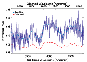
(a) 06D1bt $z=0.81$

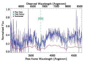
(b) 06D1bz $z=0.833$

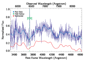
(c) 06D2ja $z=0.726$

(d) 06D2js $z=0.60$

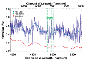
(e) 06D3ed $z=0.404$

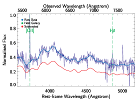
(f) 06D3el $z=0.519$

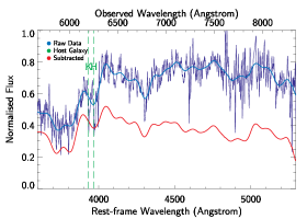
(g) 06D3et $z=0.5755$

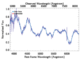
(h) 06D3fp $z=0.268$

Figure 15: Type Ia Supernovae (CI = 4 or 5)

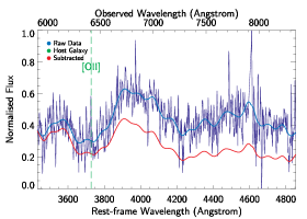
(a) 06D3gh $z=0.720$

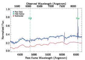
(b) 06D3gn $z=0.2501$

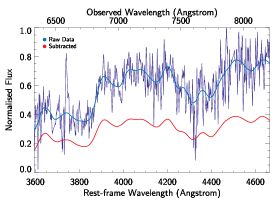
(c) 06D3gx $z=0.76$

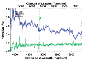
(d) 06D4dh $z=0.3027$

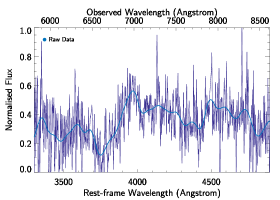
(e) 06D4dr $z=0.76$

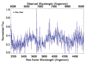
(f) 06D4fy $z=0.88$

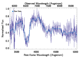
(g) 07D1cx $z=0.74$

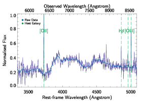
(h) 07D1ds $z=0.706$

Figure 16: Type Ia Supernovae (CI = 4 or 5)

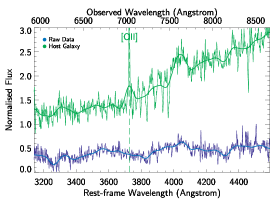
(a) 07D1dv $z=0.887$

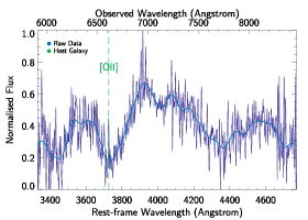
(b) 07D1ea $z=0.775$

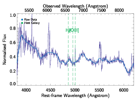
(c) 07D2kc $z=0.354$

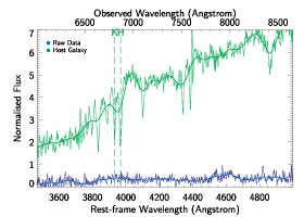
(d) 07D2kh $z=0.731$

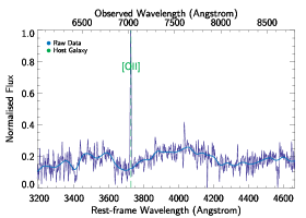
(e) 07D2cy $z=0.886$

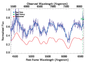
(f) 07D3ae $z=0.237$

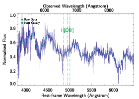
(g) 07D3af $z=0.237$

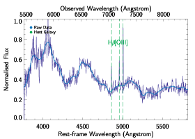
(h) 07D3ap $z=0.451$

Figure 17: Type Ia Supernovae (CI = 4 or 5)

(a) 07D3cn $z0.898$

(b) 07D3cr $z-0.746$

(c) 07D3cu $z=0.512$

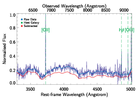
(d) 07D3da $z=0.837$

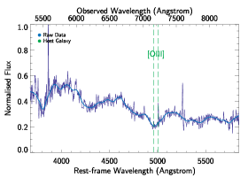
(e) 07D3dj $z=0.444$

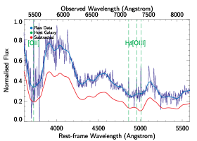
(f) 07D3ea $z=0.471$

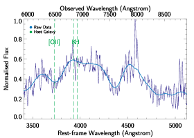
(g) 07D3ey $z=0.740$

(h) 07D3gm $z=0.83$

Figure 18: Type Ia Supernovae (CI = 4 or 5)

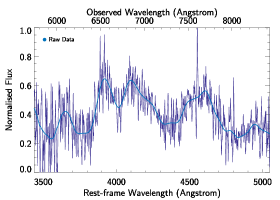
(a) 07D3hl $z=0.67$

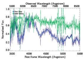
(b) 07D3hu $z=0.572$

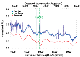
(c) 07D3hv $z=0.351$

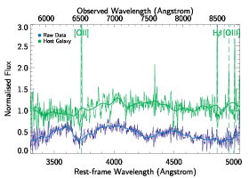
(d) 07D3hw $z=0.748$

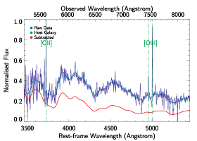
(e) 07D3hz $z=0.506$

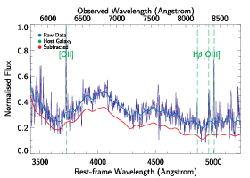
(f) 07D3ib $z=0.681$

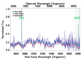
(g) 07D3it $z=0.835$

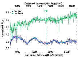
(h) 07D4fl $z=0.503$

Figure 19: Type Ia Supernovae (CI = 4 or 5)

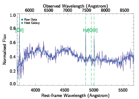
(a) 08D2aa $z=0.538$

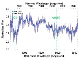
(b) 08D2ad $z=0.554$

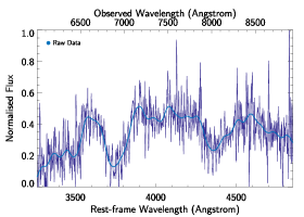
(c) 08D2bj $z=0.84$

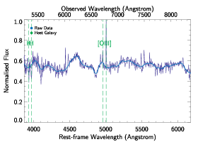
(d) 08D2dr $z=0.355$

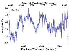
(e) 08D2dz $z=0.65$

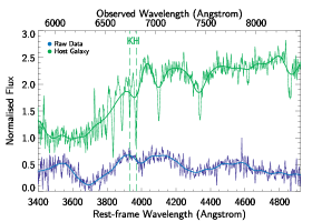
(f) 08D2gw $z=0.715$

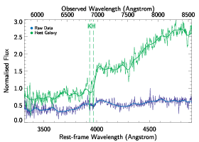
(g) 08D2hw $z=0.746$

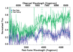
(h) 08D2id $z=0.833$

Figure 20: Type Ia Supernovae (CI = 4 or 5)

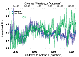
(a) 08D2iq $z=0.709$

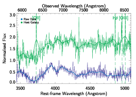
(b) 08D2kj $z=0.702$

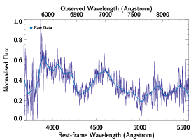
(c) 08D3bh $z=0.52$

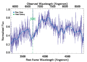
(d) 08D3dc $z=0.799$

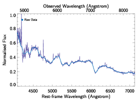
(e) 08D3gb $z=0.17$

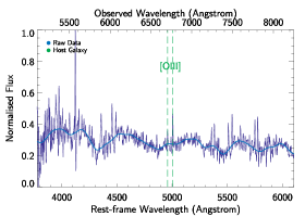
(f) 08D3gf $z=0.352$

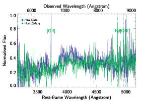
(g) 08D3gu $z=0.767$

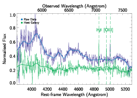
(h) 08D3hh $z=0.452$

Figure 21: Type Ia Supernovae (CI = 4 or 5)

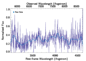
(a) 06D1ck $z=0.90$

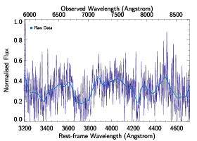
(b) 06D2iz $z=0.85$

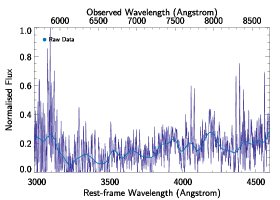
(c) 06D2ji $z=0.90$

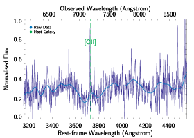
(d) 06D2ju $z=0.927$

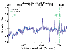
(e) 06D4fc $z=0.677$

(f) 07D3bo $z=0.92$

(g) 07D3bt $z=0.91$

(h) 07D3do $z=1.02$

Figure 22: Probable Type Ia Supernovae (CI = 3)

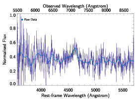
(a) 08D1aa $z=0.54$

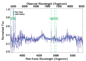
(b) 08D2ch $z=0.474$

(c) 08D2cl $z=0.831$

(d) 08D3dx $z=0.928$

Figure 23: Probable Type Ia Supernovae (CI = 3)

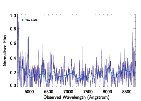
(a) 05D4bo $z$ unknown

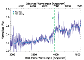
(b) 06D1gu $z=0.87$

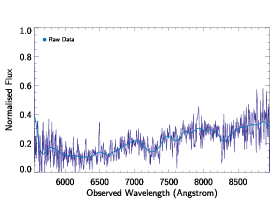
(c) 06D1hl $z$ unknown

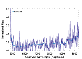
(d) 06D1jp $z$ unknown

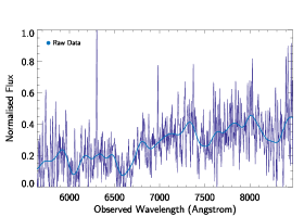
(e) 06D3fv $z$ unknown

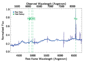
(f) 06D3hd $z=0.2409$

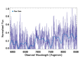
(g) 06D4gn $z$ unknown

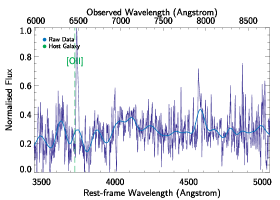
(h) 07D2bu $z=0.733$

Figure 24: Unknown (CI=2)

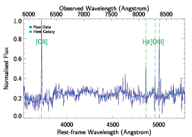
(a) 07D2ki $z=0.673$

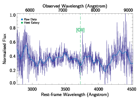
(b) 07D2kl $z=1.023$

(c) 07D3bb $z$ unknown

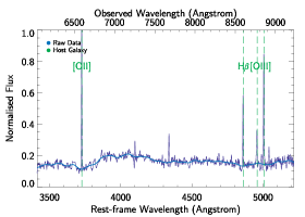
(d) 07D3bp $z=0.769$

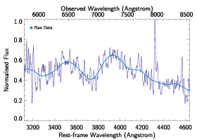
(e) 07D3fi $z$ unknown

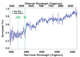
(f) 08D2au $z=0.563$

(g) 08D3fp $z$ unknown

(h) 08D3fu $z=0.426$

Figure 25: Unknown (CI=2)

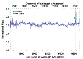
(a) 06D1dt $z=0.298$

(b) 06D1gg $z$ unknown

(c) 06D4hc $z=0.38$

(d) 07D2ke $z=0.114$

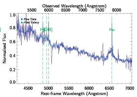
(e) 07D3ai $z=0.198$

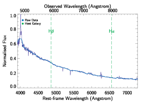
(f) 07D3am $z=0.214$

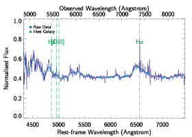
(g) 08D2eo $z=0.125$

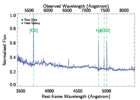
(h) 08D2fj $z=0.507$

Figure 26: Probably or Definitely Not Type Ia Supernovae (CI=1 or 0)

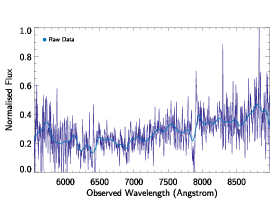
(a) 08D3au $z$ unknown

Figure 27: Probably or Definitely Not Type Ia Supernovae (CI=1 or 0)

References

- Ajhar et al. (2001) Ajhar E. A., Tonry J. L., Blakeslee J. P., Riess A. G., Schmidt B. P., 2001, ApJ, 559, 584
- Altavilla et al. (2007) Altavilla, G., Stehle, M., Ruiz-Lapuente, P., Mazzali, P., Pignata, G., Balastegui, A., Benetti, S., Blanc, G., Canal, R., Elias-Rosa, N., Goobar, A., Harutyunyan, A., Pastorello, A., Patat, F., Rich, J., Salvo, M., Schmidt, B. P., Stanishev, V., Taubenberger, S., Turatto, M., Hillebrandt, W., 2007, A&A, 475, 585
- Anupama, Sahu & Jose (2005) Anupama G. C., Sahu D. K., Jose J., 2005, A&A, 429, 667
- Appenzeller et al. (1998) Appenzeller I., Fricke K., Fürtig W., Gässler W., Häfner R., Harke R., Hess H.-J., Hummel W., Jürgens P., Kudritzki R.-P., Mantel K.-H., Meisl W., Muschielok B., Nicklas H., Rupprecht G., Seifert W., Stahl O., Szeifert T., Tarantik K., 1998, ESO Messenger, 94, 1
- Arnett (1979) Arnett W. D., 1979, ApJ, 230, L37
- Arnett (1982) Arnett W. D., 1982, ApJ, 253, 785
- Astier et al. (2006) Astier P., Guy J., Regnault N., Pain R., Aubourg E., Balam D., Basa S., Carlberg R. G., Fabbro S., Fouchez D., Hook I. M., Howell D. A., Lafoux H., Neill J. D., Palanque-Delabrouille N., Perrett K., Pritchet C. J., Rich J., Sullivan M., Taillet R., Aldering G., Antilogus P., Arsenijevic V., Balland C., Baumont S., Bronder J., Courtois H., Ellis R. S., Filiol M., Gonçalves A. C., Goobar A., Guide D., Hardin D., Lusset V., Lidman C., McMahon R., Mouchet M., Mourao A., Perlmutter S., Ripoche P., Tao C., Walton N., 2006, A&A, 447, 31
- Bailey et al. (2009) Bailey S., Aldering G., Antilogus P., Aragon C., Baltay C., Bongard S., Buton C., Childress M., Chotard N., Copin Y., Gangler E., Loken S., Nugent P., Pain R., Pecontal E., Pereira R., Perlmutter S., Rabinowitz D., Rigaudier G., Runge K., Scalzo R., Smadja G., Swift H., Tao C., Thomas R. C., Wu C., Factory T. N. S., 2009, A&A, 500, L17
- Balland et al. (2009) Balland C., Baumont S., Basa S., Mouchet M., Howell D. A., Astier P., Carlberg R. G., Conley A., Fouchez D., Guy J., Hardin D., Hook I. M., Pain R., Perrett K., Pritchet C. J., Regnault N., Rich J., Sullivan M., Antilogus P., Arsenijevic V., Du J. L., Fabbro S., Lidman C., Mourão A., Palanque-Delabrouille N., Pécontal E., Ruhlmann-Kleider V., 2009, A&A, 507, 85
- Barbon et al. (1990) Barbon R., Benetti S., Rosino L., Cappellaro E., Turatto M., 1990, A&A, 237, 79
- Baumont et al. (2008) Baumont S., Balland C., Astier P., Guy J., Hardin D., Howell D. A., Lidman C., Mouchet M., Pain R., Regnault N., 2008, A&A, 491, 567
- Benetti et al. (2005) Benetti S., Cappellaro E., Mazzali P. A., Turatto M., Altavilla G., Bufano F., Elias-Rosa N., Kotak R., Pignata G., Salvo M., Stanishev V., 2005, ApJ, 623, 1011
- Benetti et al. (2004) Benetti S., Meikle P., Stehle M., Altavilla G., Desidera S., Folatelli G., Goobar A., Mattila S., Mendez J., Navasardyan H., Pastorello A., Patat F., Riello M., Ruiz-Lapuente P., Tsvetkov D., Turatto M., Mazzali P., Hillebrandt W., 2004, MNRAS, 348, 261
- Blondin et al. (2006) Blondin S., Dessart L., Leibundgut B., Branch D., Höflich P., Tonry J. L., Matheson T., Foley R. J., Chornock R., Filippenko A. V., Sollerman J., Spyromilio J., Kirshner R. P., Wood-Vasey W. M., Clocchiatti A., Aguilera C., Barris B., Becker A. C., Challis P., Covarrubias R., Davis T. M., Garnavich P., Hicken M., Jha S., Krisciunas K., Li W., Miceli A., Miknaitis G., Pignata G., Prieto J. L., Rest A., Riess A. G., Salvo M. E., Schmidt B. P., Smith R. C., Stubbs C. W., Suntzeff N. B., 2006, AJ, 131, 1648
- Branch et al. (2006) Branch D., Dang L. C., Hall N., Ketchum W., Melakayil M., Parrent J., Troxel M. A., Casebeer D., Jeffery D. J., Baron E., 2006, PASP, 118, 560
- Branch et al. (2003) Branch D., Garnavich P., Matheson T., Baron E., Thomas R. C., Hatano K., Challis P., Jha S., Kirshner R. P., 2003, AJ, 126, 1489
- Bronder et al. (2008) Bronder T. J., Hook I. M., Astier P., Balam D., Balland C., Basa S., Carlberg R. G., Conley A., Fouchez D., Guy J., Howell D. A., Neill J. D., Pain R., Perrett K., Pritchet C. J., Regnault N., Sullivan M., Baumont S., Fabbro S., Filliol M., Perlmutter S., Ripoche P., 2008, A&A, 477, 717
- Calzetti et al. (1994) Calzetti D., Kinney A. L., Storchi-Bergmann T., 1994, ApJ, 429, 582
- Cardelli et al. (1989) Cardelli J. A., Clayton G. C., Mathis J. S., 1989, ApJ, 345, 245
- Colgate & McKee (1969) Colgate S. A., McKee C., 1969, ApJ, 157, 623
- Conley et al. (2007) Conley A., Carlberg R. G., Guy J., Howell D. A., Jha S., Riess A. G., Sullivan M., 2007, ApJ, 664, L13
- Conley et al. (2006) Conley A., Howell D. A., Howes A., Sullivan M., Astier P., Balam D., Basa S., Carlberg R. G., Fouchez D., Guy J., Hook I., Neill J. D., Pain R., Perrett K., Pritchet C. J., Regnault N., Rich J., Taillet R., Aubourg E., Bronder J., Ellis R. S., Fabbro S., Filiol M., Borgne D. L., Palanque-Delabrouille N., Perlmutter S., Ripoche P., 2006, AJ, 132, 1707
- Conley et al. (2008) Conley A., Sullivan M., Hsiao E. Y., Guy J., Astier P., Balam D., Balland C., Basa S., Carlberg R. G., Fouchez D., Hardin D., Howell D. A., Hook I. M., Pain R., Perrett K., Pritchet C. J., Regnault N., 2008, ApJ, 681, 482
- Ellis et al. (2008) Ellis R. S., Sullivan M., Nugent P. E., Howell D. A., Gal-Yam A., Astier P., Balam D., Balland C., Basa S., Carlberg R. G., Conley A., Fouchez D., Guy J., Hardin D., Hook I., Pain R., Perrett K., Pritchet C. J., Regnault N., 2008, ApJ, 674, 51
- Filippenko (1982) Filippenko A. V., 1982, Astronomical Society of the Pacific, 94, 715
- Filippenko et al. (1992) Filippenko A. V., Richmond M. W., Branch D., Gaskell M., Herbst W., Ford C. H., Treffers R. R., Matheson T., Ho L. C., Dey A., Sargent W. L. W., Small T. A., van Breugel W. J. M., 1992, AJ, 104, 1543
- Filippenko et al. (1992) Filippenko A. V., Richmond M. W., Matheson T., Shields J. C., Burbidge E. M., Cohen R. D., Dickinson M., Malkan M. A., Nelson B., Pietz J., Schlegel D., Schmeer P., Spinrad H., Steidel C. C., Tran H. D., Wren W., 1992, ApJ, 384, L15
- Fioc & Rocca-Volmerange (1997) Fioc M., Rocca-Volmerange B., 1997, A&A, 326, 950
- Fioc & Rocca-Volmerange (1999) Fioc M., Rocca-Volmerange B., 1999, eprint arXiv, astroph/9912179
- Folatelli (2004) Folatelli G., 2004, PhD Thesis
- Foley et al. (2008) Foley R. J., Filippenko A. V., Aguilera C., Becker A. C., Blondin S., Challis P., Clocchiatti A., Covarrubias R., Davis T. M., Garnavich P. M., Jha S. W., Kirshner R. P., Krisciunas K., Leibundgut B., Li W., Matheson T., Miceli A., Miknaitis G., Pignata G., Rest A., Riess A. G., Schmidt B. P., Smith R. C., Sollerman J., Spyromilio J., Stubbs C. W., Suntzeff N. B., Tonry J. L., Wood-Vasey W. M., Zenteno A., 2008, ApJ, 684, 68
- Garavini et al. (2004) Garavini G., Folatelli G., Goobar A., Nobili S., Aldering G., Amadon A., Amanullah R., Astier P., Balland C., Blanc G., Burns M. S., Conley A., Dahlén T., Deustua S. E., Ellis R., Fabbro S., Fan X., Frye B., Gates E. L., Gibbons R., Goldhaber G., Goldman B., Groom D. E., Haissinski J., Hardin D., Hook I. M., Howell D. A., Kasen D., Kent S., Kim A. G., Knop R. A., Lee B. C., Lidman C., Mendez J., Miller G. J., Moniez M., Mourão A., Newberg H., Nugent P. E., Pain R., Perdereau O., Perlmutter S., Prasad V., Quimby R., Raux J., Regnault N., Rich J., Richards G. T., Ruiz-Lapuente P., Sainton G., Schaefer B. E., Schahmaneche K., Smith E., Spadafora A. L., Stanishev V., Walton N. A., Wang L., Wood-Vasey W. M., 2004, AJ, 128, 387
- Garavini et al. (2007) Garavini G., Folatelli G., Nobili S., Aldering G., Amanullah R., Antilogus P., Astier P., Blanc G., Bronder T., Burns M. S., Conley A., Deustua S. E., Doi M., Fabbro S., Fadeyev V., Gibbons R., Goldhaber G., Goobar A., Groom D. E., Hook I., Howell D. A., Kashikawa N., Kim A. G., Kowalski M., Kuznetsova N., Lee B. C., Lidman C., Mendez J., Morokuma T., Motohara K., Nugent P. E., Pain R., Perlmutter S., Quimby R., Raux J., Regnault N., Ruiz-Lapuente P., Sainton G., Schahmaneche K., Smith E., Spadafora A. L., Stanishev V., Thomas R. C., Walton N. A., Wang L., Wood-Vasey W. M., Yasuda N., 2007, A&A, 470, 411
- Glazebrook & Bland-Hawthorn (2001) Glazebrook K., Bland-Hawthorn J., 2001, PASP, 113, 197
- Guy et al. (2007) Guy J., Astier P., Baumont S., Hardin D., Pain R., Regnault N., Basa S., Carlberg R. G., Conley A., Fabbro S., Fouchez D., Hook I. M., Howell D. A., Perrett K., Pritchet C. J., Rich J., Sullivan M., Antilogus P., Aubourg E., Bazin G., Bronder J., Filiol M., Palanque-Delabrouille N., Ripoche P., Ruhlmann-Kleider V., 2007, A&A, 466, 11
- Guy et al. (2005) Guy J., Astier P., Nobili S., Regnault N., Pain R., 2005, A&A, 443, 781
- Hamuy et al. (2002) Hamuy M., Maza J., Pinto P. A., Phillips M. M., Suntzeff N. B., Blum R. D., Olsen K. A. G., Pinfield D. J., Ivanov V. D., Augusteijn T., Brillant S., Chadid M., Cuby J.-G., Doublier V., Hainaut O. R., Floc’h E. L., Lidman C., Petr-Gotzens M. G., Pompei E., Vanzi L., 2002, AJ, 124, 417
- Höflich et al. (1998) Höflich P., Wheeler J. C., Thielemann F. K., 1998, ApJ, 495, 617
- Hook et al. (2005) Hook I. M., Howell D. A., Aldering G., Amanullah R., Burns M. S., Conley A., Deustua S. E., Ellis R., Fabbro S., Fadeyev V., Folatelli G., Garavini G., Gibbons R., Goldhaber G., Goobar A., Groom D. E., Kim A. G., Knop R. A., Kowalski M., Lidman C., Nobili S., Nugent P. E., Pain R., Pennypacker C. R., Perlmutter S., Ruiz-Lapuente P., Sainton G., Schaefer B. E., Smith E., Spadafora A. L., Stanishev V., Thomas R. C., Walton N. A., Wang L., Wood-Vasey W. M., 2005, AJ, 130, 2788
- Hook et al. (2004) Hook I. M., Jørgensen I., Allington-Smith J. R., Davies R. L., Metcalfe N., Murowinski R. G., Crampton D., 2004, PASP, 116, 425
- Howell & Nugent (2004) Howell A., Nugent P., 2004, in Cosmic Explosions in Three Dimensions, Broad Lightcurve SNe Ia: Asymmetry or Something Else? p. 151
- Howell et al. (2007) Howell D. A., Sullivan M., Conley A., Carlberg R., 2007, ApJ, 667, L37
- Howell et al. (2006) Howell D. A., Sullivan M., Nugent P. E., Ellis R. S., Conley A. J., Borgne D. L., Carlberg R. G., Guy J., Balam D., Basa S., Fouchez D., Hook I. M., Hsiao E. Y., Neill J. D., Pain R., Perrett K. M., Pritchet C. J., 2006, Nature, 443, 308
- Howell et al. (2005) Howell D. A., Sullivan M., Perrett K., Bronder T. J., Hook I. M., Astier P., Aubourg E., Balam D., Basa S., Carlberg R. G., Fabbro S., Fouchez D., Guy J., Lafoux H., Neill J. D., Pain R., Palanque-Delabrouille N., Pritchet C. J., Regnault N., Rich J., Taillet R., Knop R., McMahon R. G., Perlmutter S., Walton N. A., 2005, ApJ, 634, 1190
- Jha et al. (1998) Jha S., Garnavich P. M., Challis P. M., Kirshner R. P., Riess A. G., Filippenko A. V., Li W., Modjaz M., Treffers R. R., Grebel E. K., Seitzer P., Jacoby G. H., Benson P. J., Rizvi A., Marschall L. A., 1998, American Astronomical Society, 193, 1409
- Jha et al. (2007) Jha S., Riess A. G., Kirshner R. P., 2007, ApJ, 659, 122
- Kasen (2006) Kasen D., 2006, ApJ, 649, 939
- Keller et al. (2007) Keller, S. C., Schmidt, B. P., Bessell, M. S., Conroy, P. G., Francis, P., Granlund, A., Kowald, E., Oates, A. P., Martin-Jones, T., Preston, T., Tisserand, P., Vaccarella, A., Waterson, M. F., 2007, Publications of the Astronomical Society of Australia, 24, 1
- Kotak et al. (2005) Kotak R., Meikle W. P. S., Pignata G., Stehle M., Smartt S. J., Benetti S., Hillebrandt W., Lennon D. J., Mazzali P. A., Patat F., Turatto M., 2005, A&A, 436, 1021
- Krisciunas et al. (2007) Krisciunas K., Garnavich P. M., Stanishev V., Suntzeff N. B., Prieto J. L., Espinoza J., Gonzalez D., Salvo M. E., de la Rosa N. E., Smartt S. J., Maund J. R., Kudritzki R.-P., 2007, AJ, 133, 58
- Law et al. (2009) Law N. M., Kulkarni S. R., Dekany R. G., Ofek E. O., Quimby R. M., Nugent P. E., Surace J., Grillmair C. C., Bloom J. S., Kasliwal M. M., Bildsten L., Brown T., Cenko S. B., Ciardi D., Croner E., Djorgovski S. G., van Eyken J. C., Filippenko A. V., Fox D. B., Gal-Yam A., Hale D., Hamam N., Helou G., Henning J. R., Howell D. A., Jacobsen J., Laher R., Mattingly S., McKenna D., Pickles A., Poznanski D., Rahmer G., Rau A., Rosing W., Shara M., Smith R., Starr D., Sullivan M., Velur V., Walters R. S., Zolkower J., 2009, PASP, 121, 1395
- Leibundgut et al. (1991) Leibundgut B., Kirshner R. P., Filippenko A. V., Shields J. C., Foltz C. B., Phillips M. M., Sonneborn G., 1991, ApJ, 371, L23
- Lentz et al. (2000) Lentz E. J., Baron E., Branch D., Hauschildt P. H., Nugent P. E., 2000, ApJ, 530, 966
- Mannucci et al. (2006) Mannucci F., della Valle M., Panagia N., 2006, MNRAS, 370, 773
- Mannucci et al. (2005) Mannucci F., della Valle M., Panagia N., Cappellaro E., Cresci G., Maiolino R., Petrosian A., Turatto M., 2005, A&A, 433, 807
- Markwardt (2008) Markwardt C. B., 2008, in Astronomical Data Analysis Software and Systems XVIII, Non-Linear Least Squares Fitting in IDL with MPFIT, p251
- Matheson et al. (2008) Matheson T., Kirshner R. P., Challis P., Jha S., Garnavich P. M., Berlind P., Calkins M. L., Blondin S., Balog Z., Bragg A. E., Caldwell N., Concannon K. D., Falco E. E., Graves G. J. M., Huchra J. P., Kuraszkiewicz J., Mader J. A., Mahdavi A., Phelps M., Rines K., Song I., Wilkes B. J., 2008, AJ, 135, 1598
- Mazzali et al. (1993) Mazzali P. A., Lucy L. B., Danziger I. J., Gouiffes C., Cappellaro E., Turatto M., 1993, A&A, 269, 423
- Nugent et al. (2002) Nugent P., Kim A., Perlmutter S., 2002, PASP, 114, 803
- Pastorello et al. (2007) Pastorello A., Mazzali P. A., Pignata G., Benetti S., Cappellaro E., Filippenko A. V., Li W., Meikle W. P. S., Arkharov A. A., Blanc G., Bufano F., Derekas A., Dolci M., Elias-Rosa N., Foley R. J., Ganeshalingam M., Harutyunyan A., Kiss L. L., Kotak R., Larionov V. M., Lucey J. R., Napoleone N., Navasardyan H., Patat F., Rich J., Ryder S. D., Salvo M., Schmidt B. P., Stanishev V., Székely P., Taubenberger S., Temporin S., Turatto M., Hillebrandt W., 2007, MNRAS, 377, 1531
- Patat et al. (1996) Patat F., Benetti S., Cappellaro E., Danziger I. J., della Valle M., Mazzali P. A., Turatto M., 1996, MNRAS, 278, 111
- Perlmutter et al. (1999) Perlmutter S., Aldering G., Goldhaber G., Knop R. A., Nugent P., Castro P. G., Deustua S., Fabbro S., Goobar A., Groom D. E., Hook I. M., Kim A. G., Kim M. Y., Lee J. C., Nunes N. J., Pain R., Pennypacker C. R., Quimby R., Lidman C., Ellis R. S., Irwin M., McMahon R. G., Ruiz-Lapuente P., Walton N., Schaefer B., Boyle B. J., Filippenko A. V., Matheson T., Fruchter A. S., Panagia N., Newberg H. J. M., Couch W. J., Supernova Cosmology Project., 1999, ApJ, 517, 565
- Perlmutter et al. (1997) Perlmutter S., Gabi S., Goldhaber G., Goobar A., Groom D. E., Hook I. M., Kim A. G., Kim M. Y., Lee J. C., Pain R., Pennypacker C. R., Small I. A., Ellis R. S., McMahon R. G., Boyle B. J., Bunclark P. S., Carter D., Irwin M. J., Glazebrook K., Newberg H. J. M., Filippenko A. V., Matheson T., Dopita M., Couch W. J., The Supernova Cosmology Project, 1997, ApJ, 483, 565
- Phillips (1993) Phillips M. M., 1993, ApJ, 413, L105
- Riess et al. (1998) Riess A. G., Filippenko A. V., Challis P., Clocchiatti A., Diercks A., Garnavich P. M., Gilliland R. L., Hogan C. J., Jha S., Kirshner R. P., Leibundgut B., Phillips M. M., Reiss D., Schmidt B. P., Schommer R. A., Smith R. C., Spyromilio J., Stubbs C., Suntzeff N. B., Tonry J., 1998, AJ, 116, 1009
- Riess et al. (1996) Riess A. G., Press W. H., Kirshner R. P., 1996, AJ, 473, 88
- Riess et al. (2007) Riess A. G., Strolger L.-G., Casertano S., Ferguson H. C., Mobasher B., Gold B., Challis P. J., Filippenko A. V., Jha S., Li W., Tonry J., Foley R., Kirshner R. P., Dickinson M., MacDonald E., Eisenstein D., Livio M., Younger J., Xu C., Dahlen T., Stern D., 2007, ApJ, 659, 98
- Saha et al. (2006) Saha A., Thim F., Tammann G. A., Reindl B., Sandage A., 2006, ApJS, 165, 108
- Salvo et al. (2001) Salvo M. E., Cappellaro E., Mazzali P. A., Benetti S., Danziger I. J., Patat F., Turatto M., 2001, MNRAS, 321, 254
- Savitzky & Golay (1964) Savitzky A., Golay M. J. E., 1964, Analytical Chemistry, 36, 1627
- Scannapieco & Bildsten (2005) Scannapieco E., Bildsten L., 2005, ApJ, 629, L85
- Schlegel et al. (1998) Schlegel D. J., Finkbeiner D. P., Davis M., 1998, ApJ, 500, 525
- Stanishev et al. (2007) Stanishev V., Goobar A., Benetti S., Kotak R., Pignata G., Navasardyan H., Mazzali P., Amanullah R., Garavini G., Nobili S., Qiu Y., Elias-Rosa N., Ruiz-Lapuente P., Mendez J., Meikle P., Patat F., Pastorello A., Altavilla G., Gustafsson M., Harutyunyan A., Iijima T., Jakobsson P., Kichizhieva M. V., Lundqvist P., Mattila S., Melinder J., Pavlenko E. P., Pavlyuk N. N., Sollerman J., Tsvetkov D. Y., Turatto M., Hillebrandt W., 2007, A&A, 469, 645
- Sullivan et al. (2006) Sullivan M., Borgne D. L., Pritchet C. J., Hodsman A., Neill J. D., Howell D. A., Carlberg R. G., Astier P., Aubourg E., Balam D., Basa S., Conley A., Fabbro S., Fouchez D., Guy J., Hook I., Pain R., Palanque-Delabrouille N., Perrett K., Regnault N., Rich J., Taillet R., Baumont S., Bronder J., Ellis R. S., Filiol M., Lusset V., Perlmutter S., Ripoche P., Tao C., 2006, ApJ, 648, 868
- Sullivan et al. (2009) Sullivan M., Ellis R. S., Howell D. A., Riess A., Nugent P. E., Gal-Yam A., 2009, ApJL, 693, L76
- Valentini et al. (2003) Valentini G., Carlo E. D., Massi F., Dolci M., Arkharov A. A., Larionov V. M., Pastorello A., Paola A. D., Benetti S., Cappellaro E., Turatto M., Pedichini F., D’Alessio F., o Garatti A. C., Causi G. L., Speziali R., Danziger I. J., Tornambé A., 2003, ApJ, 595, 779
- Wang et al. (2003) Wang L., Goldhaber G., Aldering G., Perlmutter S., 2003, ApJ, 590, 944
- Wood-Vasey et al. (2007) Wood-Vasey W. M., Miknaitis G., Stubbs C. W., Jha S., Riess A. G., Garnavich P. M., Kirshner R. P., Aguilera C., Becker A. C., Blackman J. W., Blondin S., Challis P., Clocchiatti A., Conley A., Covarrubias R., Davis T. M., Filippenko A. V., Foley R. J., Garg A., Hicken M., Krisciunas K., Leibundgut B., Li W., Matheson T., Miceli A., Narayan G., Pignata G., Prieto J. L., Rest A., Salvo M. E., Schmidt B. P., Smith R. C., Sollerman J., Spyromilio J., Tonry J. L., Suntzeff N. B., Zenteno A., 2007, ApJ, 666, 694