Forward modelling to determine the observational signatures of white-light imaging and interplanetary scintillation for the propagation of an interplanetary shock in the ecliptic plane

Abstract

Recent coordinated observations of interplanetary scintillation (IPS) from the EISCAT, MERLIN, and STELab, and stereoscopic white-light imaging from the two heliospheric imagers (HIs) onboard the twin STEREO spacecraft are significant to continuously track the propagation and evolution of solar eruptions throughout interplanetary space. In order to obtain a better understanding of the observational signatures in these two remote-sensing techniques, the magnetohydrodynamics of the macro-scale interplanetary disturbance and the radio-wave scattering of the micro-scale electron-density fluctuation are coupled and investigated using a newly-constructed multi-scale numerical model. This model is then applied to a case of an interplanetary shock propagation within the ecliptic plane. The shock could be nearly invisible to an HI, once entering the Thomson-scattering sphere of the HI. The asymmetry in the optical images between the western and eastern HIs suggests the shock propagation off the Sun-Earth line. Meanwhile, an IPS signal, strongly dependent on the local electron density, is insensitive to the density cavity far downstream of the shock front. When this cavity (or the shock nose) is cut through by an IPS ray-path, a single speed component at the flank (or the nose) of the shock can be recorded; when an IPS ray-path penetrates the sheath between the shock nose and this cavity, two speed components at the sheath and flank can be detected. Moreover, once a shock front touches an IPS ray-path, the derived position and speed at the irregularity source of this IPS signal, together with an assumption of a radial and constant propagation of the shock, can be used to estimate the later appearance of the shock front in the elongation of the HI field of view. The results of synthetic measurements from forward modelling are helpful in inferring the in-situ properties of coronal mass ejection from real observational data via an inverse approach.

1 Introduction

1.1 Interplanetary Space

Interplanetary space can be considered as a transmission channel connecting the Sun and the Earth, permeated with the ubiquitous magnetized solar wind flow from the Sun. The solar wind is inherently bimodal with fast solar wind from coronal holes and slow solar wind above coronal streamers (McComas et al., 2000). As a consequence of the root of the spiral interplanetary magnetic field (IMF) on the rotating Sun, the interface between the fast and slow solar winds at the same latitude gradually develops into a co-rotating interaction region (CIR) with increasing heliocentric distance. The ambient radial plasma flow in the co-rotating inhomogeneous background structure is frequently interrupted by coronal mass ejections (CMEs). A CME could undergo significant, nonlinear, and irreversible evolution during its interplanetary propagation, interacting with the ambient structured medium and other CMEs. An individual CME could have its outer magnetic shell stripped away to form a diffusive boundary layer by magnetic reconnection (Wei et al., 2006), be significantly pushed at its rear boundary by a CIR (Dal Lago et al., 2006), and even be entrained by a CIR (Rouillard et al., 2009). The coupling of multiple CMEs in the Sun-Earth system could result in a complex ejecta (Burlaga et al., 2002) or a shock-penetrated magnetic cloud (MC) (Lepping et al., 1997). Particularly, the compression effect accompanying CMEs colliding can intensify the southward magnetic field and is subsequently responsible for major geomagnetic storms (Burlaga et al., 1987). In terms of space weather, interplanetary space should be emphasized as a pivotal node in the development of the solar-terrestrial causal process.

1.2 Remote-Sensing Techniques

The interplanetary space environment has been sampled frequently by observing interplanetary scintillation (IPS) of radio waves, beginning with the pioneering work of Hewish et al. (1964). IPS is essentially the intensity scintillation received at a terrestrial radio antenna as a result of a drifting interference pattern across the IPS ray-path, formed by density fluctuations in the solar wind. The intensity variance on the time-scale of 0.1 $\sim$ 10 seconds for the micro-scale density irregularities, with a characteristic scale of tens to a few hundreds of kilometers, can be sequentially recorded by two telescopes if the baseline between two telescopes is basically parallel to the drifting speed of density irregularities (Bisi, 2006). Long baselines can resolve multiple solar wind streams crossing the IPS ray-path, which contribute to the integral intensity towards the Earth from the different radio-scattering layers along the IPS ray-path. The stream interface could be a shear and sliding layer between a fast stream at the high latitude and a slow stream at the ecliptic plane, or a compression layer within the CIR, as the IPS observations reveal the velocity gradient and normal scintillation level for the sliding layer, and an intermediate velocity and enhanced scintillation level for the compression layer (Bisi et al., 2010). The presence of a CME amid the background of bimodal solar-wind streams (Dorrian et al., 2008) can be identified from the IPS signal as (1) a noticeable negative lobe in the cross-correlation function (CCF), (2) a rapid variation of the solar wind speed, the CCF shape, and the scintillation level on the time-scale of hours or less. The poleward deflection of the ambient solar wind ahead of a CME on 13 May 2005 (Breen et al., 2008) and the micro-structure of two CMEs merging on 16 May 2007 (Dorrian et al., 2008) were reported by the IPS observations, using the European Incoherent SCATter radar (EISCAT) in northern Scandinavia, the Multi-Element Radio-Linked Interferometer Network (MERLIN) radio telescopes in United Kingdom, and the Solar-Terrestrial Environment Laboratory (STELab) in Japan. The capability of the traditional and economical IPS technique to probe the inner heliosphere has been significantly improved by the current advances of long baselines of over 2000 km, the single observing frequency of around 1.4 GHz, and dual-frequency observations of IPS (Fallows et al., 2006).

Modern heliospheric imaging and the traditional IPS techniques can routinely cover the whole interplanetary space to fill in the relative observation data gap between the comprehensively monitored Sun and Earth. On the one hand, stereoscopic optical observations using Heliospheric Imagers (HIs) (Howard et al., 2008; Eyles et al., 2009) have been successfully realized as a major milestone since the launch of the twin Solar Terrestrial Relations Observatory (STEREO) spacecraft in 2006 (Kaiser, 2008). Occupying solar orbits approximately at 1 AU, the STEREO A leads the Earth in the west and the STEREO B lags the Earth in the east. Both STEREO A and B are separated from the Earth by $22.5^{\circ}$ per year. Onboard either STEREO spacecraft, each HI instrument comprises two cameras of HI-1 and HI-2, whose optical axes lie in the ecliptic plane. Seen from a spacecraft, an angular distance between the Sun and a target is defined by an elongation. The elongation coverage is $4^{\circ}\sim 24^{\circ}$ for the HI-1 and $18.7^{\circ}\sim 88.7^{\circ}$ for the HI-2; the field of view (FOV) is $20^{\circ}\times 20^{\circ}$ for the HI-1 and $70^{\circ}\times 70^{\circ}$ for the HI-2; the time cadence is 40 minutes for the HI-1 and 2 hours for the HI-2 (Howard et al., 2008; Eyles et al., 2009). For HI imaging, the transient brightness of electron-scattered sunlight is blended with the stable brightness of dust-scattered sunlight, star light, and planet light. Subtracted from the background brightness, a white-light image could be discernible for the sunlight-illuminated interplanetary transients. One or two vantage views from HI imaging can not only recognize the background brightness of a CIR (Rouillard et al., 2008; Sheeley et al., 2008), but also track the speed, trajectory, and shape of interplanetary transients (Davies et al., 2009; Webb et al., 2009). An Earth-directed MC and its possible interaction with another MC or an incident shock could be expected to be directly imaged in interplanetary space. The visibility of potentially geoeffective complicated structures such as MC-shock interaction (Xiong et al., 2006a, b) and MC-MC collision (Xiong et al., 2007, 2009; Lugaz et al., 2009) in the FOV of an HI can give an early warning of a space weather event before its ultimate arrival at 1 AU and hence at the Earth. On the other hand, STElab IPS data can be employed to generate a tomographic reconstruction of the three-dimensional large-scale solar wind density (Jackson et al., 2003), as applied to the constraints of IPS data from the EISCAT and MERLIN (Breen et al., 2008), and the comparisons with density images from the Solar Mass Ejection Imager (SMEI) (Bisi et al., 2008). When an IPS ray-path lies within the FOV of an HI, the joint observations record simultaneous multi-scale manifestations for interplanetary dynamics, as demonstrated in the study of the merging between two converging CMEs on 16 May 2007 (Dorrian et al., 2008). In addition, as the optical imaging from a single HI only records the horizontal and vertical motions of a CME, the extra depth information could be complemented by the line of sight (LOS) at a different perspective from another HI or from IPS. Thus, the coordinated remote-sensing observations using both HI and IPS cover a wide range of heliocentric distances and almost all heliographic latitudes at any time, and record the consistent multi-scale responses in white-light and radio wave scintillation to the interplanetary passage of a CME.

1.3 Observations and Models

The interpretation of HI and IPS observational data relies significantly on theoretical modelling, since the models provide an insight into the underlying physical processes from its observable manifestation in the electromagnetic spectrum. For the integral signal along an IPS ray-path, the ambiguity of its LOS distribution is usually limited and removed by the addition of solar corona observations via the iterative fitting of a kinematic solar wind model (Klinglesmith, 1997). This kinematic model assumes a purely radial solar wind flow with each stream travelling at a constant velocity, and projects the IPS ray-path onto a solar source surface using a ballistic mapping along the spiral IMF at an appropriate speed. By this method, the modes of solar wind occupying different regions of the IPS ray-path can be inferred from the distribution of dark (coronal hole) and bright (streamer) regions of the corona onto which the projected ray-path falls (Klinglesmith, 1997; Bisi, 2006). Similarly, the derived distribution along the IPS ray-path constrained by the solar surface map can be further mapped outwards along the same ballistic trajectory to the positions of Ulysess at high latitude, and Wind/ACE at Earth orbit, allowing a direct comparison with the corresponding in-situ observation data (Bisi et al., 2010). The intersecting points of ballistic trajectories mapped at different speeds provide a qualitative indication of the location of the compression region within a CIR (Bisi et al., 2010). Multiple observational data at different solar distances, longitudes, and latitudes, are assumed to be causally linked via ballistic mapping in this kinematic solar wind model, so the IPS data could be fitted with the extra freedom limited by other observational data (Klinglesmith, 1997). For HI, the geometric influence of the Thomson-scattering sphere significantly affects the appearance of a CME in the FOV (Vourlidas and Howard, 2006; Howard and Tappin, 2009). During the interplanetary propagation of a CME, the relative position between the CME and the Thomson sphere changes continuously and different parts of the CME would be imaged by the HI at different times. For simultaneous stereoscopic imaging, the Thomson-scattering responses of the HI-A and HI-B could be quite asymmetrical. Moreover, the coexistence and possible interaction between the co-rotating background plasma in a CIR and the outwardly moving CME, can further complicate the interpretation of white-light images. Because of the intractable nature of analytical methods, the numerical model can assist by providing global context and hints of what can and cannot be observed in HI images (Odstrcil and Pizzo, 2009). Meanwhile, the time-dependent solution from forward modelling with a numerical heliospheric model can give the profile along any IPS ray-path. Thus, the local IPS data are assimilated into the global numerical model in a self-consistent way. Further, if an IPS model for the micro-scale scattering process is logically coupled with a heliospheric model for the macro-scale magnetohydrodynamic (MHD) context, the synthetic observation signatures of both HI and IPS can be derived from the multi-scale model and be linked to the interplanetary dynamics. Motivated by the integration of observational data as irrefutable evidence, and theoretical modelling as a convincing interpretation, we have undertaken a preliminary study in this paper of an incident shock propagation within the ecliptic plane using a newly-constructed multi-scale model. The propagation and evolution of an interplanetary CME can be better monitored and understood by the joint efforts of an inverse approach from the remote-sensing observations and a forward modelling from the numerical simulations.

In this paper, the synthetic observation signatures of white-light imaging and IPS are forwardly modelled for the propagation of an interplanetary shock within the ecliptic plane. We present the multi-scale numerical model in Section 2, describe the individual observations from the HIs in Section 3 and IPS in Section 4, analyze the correspondence and coordination of the simultaneous white-light data and IPS data for the same spatial position of interplanetary space in Section 5, and summarize this paper and discuss the potential of using the coordinated HI and IPS observations to identify a possible longitudinal deflection of a CME/Shock in Section 6.

2 A Multi-Scale Numerical Model

The observation signatures of white-light brightness and radio-wave scintillation are physically described by our newly constructed numerical model, an integration of a numerical MHD model for the macro-scale driver and an IPS model for the micro-scale response. This multi-scale model is implemented in the following steps to causally couple the multiple physical processes at dramatically different temporal and spatial scales.

The global MHD model for interplanetary space, governed by a set of ideal MHD equations (c.f. Hu, 1998), is numerically solved by a mathematical shock-capturing algorithm of Piecewise Parabolic Method with a Lagrangian remap (PPMLR) (Colella and Woodward, 1984; Hu et al., 2007). The ecliptic plane from 0.1 to 1 AU is discretized into a mesh of 200 $\times$ 360 grids with its radial spacing 0.0045 AU and longitudinal spacing $1^{\circ}$. The background solar wind is prescribed by the inner boundary conditions at 0.1 AU: number density of $8.2\times 10^{-4}$ m^-3, magnetic field of 250 nT, solar rotation speed of $2.9\times 10^{-6}$ rad s^-1, a temperature of $4.65\times 10^{5}$ K, and a bulk-flow speed of 375 km s^-1. In this model, the background solar wind is uniform along the longitudinal direction. Then, the initial equilibrium of interplanetary space is disturbed by a fast MHD shock from solar eruption, characterized by the shock nose at longitude of $45^{\circ}$, the shock front width of $30^{\circ}$, the initial shock speed $1150$ km s^-1, the total pressure ratio of 18 across the front discontinuity, the disturbance duration of 2 hours. The introduction of this shock into the simulation domain is numerically realized by the modification of the inner boundary conditions at 0.1 AU (Xiong et al., 2006a, b). Thus, the propagation and evolution of a shock wave through interplanetary space is quantitatively described in a macro-scale by the MHD model.

The synthetic white-light imaging is generated from MHD simulation data by the well-established Thomson-scattering theory (Vourlidas and Howard, 2006; Howard and Tappin, 2009). The location of the maximum scattered sunlight lies on the Thomson-scattering sphere which is centred half-way between the Sun and the observer with its diameter equal to the Sun-observer distance. The geometry factor of the Thomson-scattering sphere should be included to correctly interpret the heliospheric imaging (Vourlidas and Howard, 2006; Howard and Tappin, 2009). Both the total electron number and its position relative to the Thomson-scattering sphere significantly affect the brightness in interplanetary space. As pointed out by Howard and Tappin (2009), (1) though the Thomson scattering itself is minimized on the Thomson surface, the scattered sunlight is maximized on the Thomson surface; (2) the scattered sunlight is maximized simply because it is at the point along any LOS that is closest to the Sun, where the incident sunlight and density are greatest; (3) the scattered intensity becomes more spread out with distance from the Thomson surface. So the importance of the Thomson surface in the Vourlidas and Howard (2006) method is somewhat de-emphasized in the Howard and Tappin (2009) method. However, in this paper, only Vourlidas and Howard (2006) method is adopted for simplicity. The more sophisticated method of Howard and Tappin (2009) will be considered in our model in the future. For an interplanetary electron scattering photospheric light, the geometry sketch is illustrated by Vourlidas and Howard (2006, Figure 1), the Thomson-scattering algorithm is available as an IDL procedure “eltheory.pro” in the solar-soft library under the SOHO/LASCO directory. Hence, the propagation of interplanetary disturbances in our model directly provides their manifestation in the synthetic white-light images.

The IPS model for the local intensity modulation of radio waves makes use of a Born approximation to the general weak-scattering theory (Tatarski et al., 1993; Fallows, 2001). The spatial fluctuation of the local density irregularities at a micro-scale of about 200 km is conveyed by the ambient solar wind flow, and consequently introduces a scintillation pattern in the ($x$, $y$) plane perpendicular to the IPS ray-path along the $z$ direction. Here ($x$, $y$, $z$) is a cartesian coordinate system centred on the Earth. The amount of scintillation introduced by density irregularities in the solar wind varies according to the square of density fluctuations $\delta N_{e}^{2}$ (Salpeter, 1967). As the variation of $\delta N_{e}$ with heliocentric distance is not well determined from observations, it is a common practice in IPS studies to assume that $\delta N_{e}$ varies as $N_{e}$, as suggested by Houminer and Hewish (1972). The intensity $P_{\Delta I}$ in a total spectrum of the spatial wave vector $(k_{x},k_{y})$ is merely a linear superposition of all contributions from every thin scattering layer along the IPS ray-path connecting the Earth to a remote radio source, as described by $P_{\Delta I}(k_{x},k_{y})=\int P^{\prime}_{\Delta I}(k_{x},k_{y},z)dz$ (Klinglesmith, 1997). For each scattering layer with its thickness $dz$ at distance $z$, a linear relation between the radio intensity scintillation $P^{\prime}_{\Delta I}(k_{x},k_{y},z)$ and the spectrum of electron density irregularities, $P_{N_{e}}$, is given by the following set of mathematical expressions with the notations of the electron number density $N_{e}$, the classic electron radius $r_{e}=2.82\times 10^{-5}$ m, the observing wavelength $\lambda$, the spatial wave number $k$, the Fresnel radius $r_{f}$, the spectral exponent $\alpha$, the dissipation-associated inner scale of the sharp drop of spectral power $k_{c}$, the wave vector parallel (perpendicular) to the magnetic field $k_{\parallel}$ ($k_{\perp}$), and the axial ratio of anisotropy degree $AR$ at a heliocentric distance $r$ with its reference of $AR_{0}=8$ at $r_{0}=5$ solar radii (Coles and Harmon, 1989; Klinglesmith, 1997; Massey, 1998):

$$P^{\prime}_{\Delta I}(k_{x},k_{y},z) = 8\pi(r_{e}\lambda)^{2}\sin^{2}(\frac{|k|^{2}\lambda z}{4\pi})P_{N_{e}}(k_{x},k_{y},k_{z}=0,z)dz$$ (1)

$$r_{f} = \sqrt{\lambda z}$$ (2)

$$P_{N_{e}}(k_{x},k_{y},k_{z},z) \varpropto P_{N_{e}}(k_{\parallel},k_{\perp})\varpropto N_{e}^{2}\frac{e^{-(|k|/k_{c})^{2}}}{(k^{2}_{\parallel}+k^{2}_{\perp}/AR^{2})^{\alpha/2}}$$ (3)

$$AR = (AR_{0}-1)\cdot(r_{0}/r)^{1.3}+1$$ (4)

The cylindrically-symmetric coordinate system ($k_{\parallel},k_{\perp}$) with its axis along the local magnetic field is transferred from the coordinate system ($x,y,z$) defined with respect to the IPS ray-path. In equation (1), the term $\sin^{2}(\frac{|k|^{2}\lambda z}{4\pi})$ is a high pass Fresnel filter with its Fresnel radius $r_{f}=\sqrt{\lambda z}$. Such a radius $r_{f}$ determines the maximum scale of the irregularities, at which the amplitude fluctuation can be received at the Earth. When the spatial spectrum of intensity $P_{\Delta I}(k_{x},k_{y})$ carried by an anti-sunward speed $\mathbf{V}$ is drifted across an IPS ray-path with its intersection angle ($90^{\circ}-\theta$), only the speed component perpendicular to the IPS ray-path $|\mathbf{V}_{\mbox{\tiny drift}}|=|\mathbf{V}|\cdot\cos\theta$ is detectable by a terrestrial radio antenna. The geometry factor $\cos\theta$ varies along the entire IPS ray-path. Moreover, the nearly identical diffraction pattern of radio signatures can be sequentially received by two fixed terrestrial antennas separated by a baseline $\mathbf{b}$. If the baseline $\mathbf{b}$ on the Earth is approximately parallel to the drifting direction $\mathbf{V}_{\mbox{\tiny drift}}$ of micro-scale density irregularities in interplanetary space, the scintillation patterns at the two telescopes will be correlated with some time lag $\tau$. At any scattering layer $z$, the spatial correlation function between two antennas $R^{\prime}_{12}(\mathbf{b},\tau,z)=R^{\prime}_{12}(\mathbf{S}=\mathbf{b}-\mathbf{V}_{\mbox{\tiny drift}}\cdot\tau,z)$ can be converted from the spatial spectrum $P^{\prime}_{\Delta I}(k_{x},k_{y},z)$ via a Fourier transform. Specifically, the spatial-to-temporal conversion is merely a cut in the spatial correlation function along the direction of $\mathbf{b}-\mathbf{V}_{\mbox{\tiny drift}}\cdot\tau$. When the baseline $\mathbf{b}$ is zero, the Cross-Correlation Function (CCF) between two antennas is degenerated to the Auto-Correlation Function (ACF) for either antenna. For a single scattering layer, the CCF is simply derived by shifting the ACF at a time lag $|\mathbf{b}|/|\mathbf{V}_{\mbox{\tiny drift}}|$. Inversely, the drifting speed $\mathbf{V}_{\mbox{\tiny drift}}$ can be inferred from the time lag $\tau$, which is the principle of IPS estimation for solar wind outflow. The drift speed in the CCF of IPS signals is the manifestation of the flow speed of the local density irregularities. As the amplitude of Alfvén turbulence is much smaller in interplanetary space compared with the inner solar corona, IPS speed is likely to be close to the bulk plasma flow speed, at least in the slow solar wind (Klinglesmith, 1997). In the fast solar wind close to the Sun, IPS speeds may overestimate solar wind speeds (Klinglesmith, 1997). However, as a remote-sensing technique, an IPS signature involves the contributions from all of the scattering layers along its IPS ray-path. The ability to resolve the distribution of solar wind velocities from the cross-correlation of IPS measurements at two sites depends upon the differences in time-lags between the maxima in cross-correlation produced by different streams, and thus on the baseline length $\mathbf{b}$ and the Fresnel radius $r_{f}$ (Equation 2). In general, longer baselines improve the ability to resolve streams of different velocities (Breen et al., 2008; Bisi et al., 2010), provided that the time interval is long enough to derive well-defined scintillation spectra, when the observing geometry is suitable for cross-correlation analysis. In our IPS model, the observing wavelength (frequency) is 21 cm (1420 MHz) and the baseline $\mathbf{b}$ is 2000 km. For the radio wave at 1420 MHz, the maximum scale of the irregularity from a scattering layer at a distance of $z=$ 1 AU is 177 km. As the local IPS signature is influenced by the global parameters of bulk-flow speed, electron density, and magnetic-field orientation, synthetic IPS data can be hierarchically generated from MHD simulation data.

3 White-Light Imaging

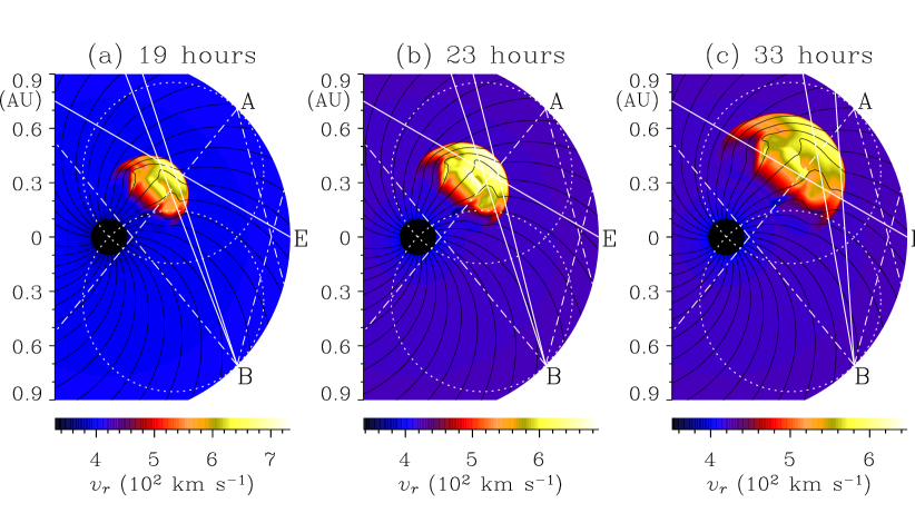
Figure 2: Radial flow speed distribution $v_{r}$ in the ecliptic plane for the propagation of an interplanetary shock at (a) 19, (b) 23, and (c) 33 hours, following its initiation.

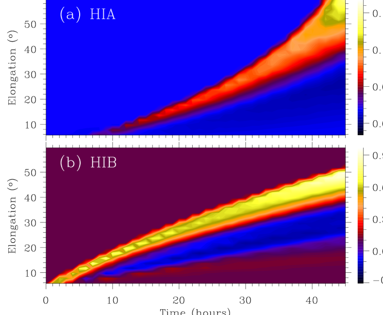
Figure 3: Relative-brightness enhancement $(I-I_{0})/I_{0}$ generated by the time-series assembling of an elongation slice within the ecliptic plane, according to synthetic data from the (a) HI-A and (b) HI-B. Here, $I_{0}$ refers to the background brightness.

The propagation of an interplanetary shock can be continuously tracked at a macro-scale by white-light imaging of the inner heliosphere. Synthetic brightness images of interplanetary disturbances can be generated from a numerical MHD model using the Thomson-scattering principle. In our model, an incident shock initially launched $45^{\circ}$ west of the Sun-Earth line, is characterized by a longitudinal width of $30^{\circ}$ along its front and a speed of 1150 km s^-1 at its nose. The time-series evolution of the shock is shown in Figure 1 for density $n$ and Figure 2 for radial speed $v_{r}$. A noticeable trailing cavity with low density is formed and expands as the shock front propagates out from the Sun. Between this so-called density cavity and the shock front lies the sheath region. Across the shock front towards the sheath, the spiral IMF lines are significantly distorted and compressed, and the bulk flow speed $v_{r}$, number density $n$, plasma temperature are abruptly enhanced. Hence the sheath downstream of a shock front is a readily observable target in interplanetary space. White-light images are simultaneously simulated for the twin HIs at points “A” and “B” in Figure 1. With the longitude of $45^{\circ}$ beside the Earth at 1 AU, any HI has the FOV from $6^{\circ}$ to $60^{\circ}$ in the elongation. From the combined views of HI-A and HI-B, the Sun-Earth line is completely covered, and interplanetary space is routinely monitored. However, the sensitivity of HI for a remote plasma parcel depends on not only its innate electron number, but also its heliographic position. Such a geometry dependence for white-light imaging arises from the Thomson-scattering process, the working principle of the HI instrument. The Thomson-scattering effect is strongest at the sphere marked by a dotted white circle in Figure 1, when the incoming direction of an incident photospheric photon is perpendicular to the outgoing scattered light towards the receiver. For the shock studied in this paper, the Thomson-scattering effect is very weak for the white light received at HI-A, as the shock propagates along the diameter of Thomson sphere of HI-A. Moreover, only the western flank of the shock front is within the HI-A’s FOV, and the distance between this shock flank and Thomson sphere is large due to the finite front width. In addition, because the LOS from HI-A penetrates both the sheath with high density and the trailing cavity with low density, the integral signal of remote sensing can only give an average effect. Therefore, the brightness of this shock in HI-A’s FOV is very faint, as shown in Figure 3. The two-dimensional time-elongation image is assembled from a series of one-dimensional slices taken at different snapshots within the ecliptic plane. This time-elongation format, widely used in the analysis of real observational data, has been shown to be very effective at revealing the evolution of solar ejecta from white-light imaging (Davis et al., 2009). Moreover, as the background brightness $I_{0}$ abruptly decreases away from the Sun, the relative-brightness enhancement $(I-I_{0})/I_{0}$ is adopted to highlight the brightness deviation from the initial steady state. The relative brightness in the HI-A’s FOV is far less than 0.1 until the shock front approaches and crosses the Thomson sphere near 1 AU. Hence the shock, heading towards the HI-A, is essentially invisible within the HI-A’s FOV. As a dramatic contrast, a bright diagonal streak is conspicuous in HI-B data with its relative brightness up to 0.9. This bright streak is immediately followed by a dark streak with a sharp boundary between them. The bright and dark features in Figure 3b correspond to the relative positions of the sheath and cavity in the HI-B FOV in Figure 1. The sheath and cavity are separately imaged via different LOSs from HI-B. The shock nose and the eastern flank are continuously detected by one varying narrow LOS band from the HI-B, whose elongation is $24^{\circ}\sim 27^{\circ}$ at 19 hours, $28^{\circ}\sim 32^{\circ}$ at 23 hours, and $35^{\circ}\sim 41^{\circ}$ at 33 hours. The asymmetry between the white-light images of the HI-A and HI-B results from the initial deviation of shock propagation from the Sun-Earth line.

With some assumptions or modelling, the spatial position of a local high-density structure could be inversely inferred from its contribution of the Thomson-scattering emission to a brightness feature in the white-light images. Once the Thomson-scattering source is pinpointed, the total electron number inside the source region can be accurately calculated from the brightness corrected by the geometry factor of the Thomson-scattering sphere. Without an additional observation limitation, the intersection point between the Thomson sphere and a LOS may be simply assumed to be the source for the corresponding bright pixel in the white-light image. This rough assumption of an interplanetary scattering source lying on the Thomson sphere suffers from a significant underestimation of total electron number. The underestimation degree has been studied for the radial propagation of a single electron at various longitudes (Vourlidas and Howard, 2006, Figure 5). Directly generating the behavior of a single propagating electron to a CME, Vourlidas and Howard (2006) found from their qualitative model that the mass underestimation (1) exceeds a factor of 2 for a limb CME at elongations larger than $60^{\circ}$, (2) also exceeds a factor of 2 for a halo CME at elongations smaller than $20^{\circ}$, and (3) is never off by more than 20% for a CME, propagating along intermediate longitudes ($\sim 40^{\circ}$), even at extreme elongations. As a contrast to the results from heliospheric imaging, the mass underestimation from the coronagraph for heliocentric distances of less than 30 solar radii is less than 50%, even when a simpler assumption is made that the electron source is solely at the so-named plane of sky perpendicular to the Sun-observer line (Vourlidas et al., 2000). Moreover, the real three-dimensional density distribution is more complex for an interplanetary propagating CME against the background of the ambient bimodal solar wind, which is difficult to retrieve from white-light imaging. A more realistic investigation has to resort to numerical simulations, particularly for the explanation of a practical observation event. Though the outline of an interplanetary CME in the white-light image can be easily identified by the excess brightness of CME images subtracted from a pre-event background image, the conversion from such an excess brightness to the actual mass is not straightforward. Simultaneous imaging from two vantage points of the twin STEREO spacecraft can significantly improve the capability of identifying the spatial location of electron source for an Earth-directed halo CME. However, when a front-side CME propagates off the Sun-Earth line and fully enters the Thomson sphere of one HI, only the other HI can discern the CME-driven shock front, as demonstrated in Figures 1 and 3 of this paper. Therefore, in order to reduce the ambiguity of interpretation for the observation data of STEREO HI-A and HI-B, some additional observation techniques are necessary to provide some further observational constraints.

4 Interplanetary Scintillation Signal

Measurements of radio scintillation can provide a way of probing the physical processes at a micro-scale of $\sim$ 200 km, such as the electron density, bulk flow speed, magnetic-field direction, and level of Alfvénic turbulence. Because an IPS signal is roughly proportional to the square of electron density (equation 3) and an HI signal depends linearly on the electron density, the IPS signal is even more sensitive to high density regions of solar wind. When the tiny source of a strong IPS signal is located in the bright domain of HI imaging, the IPS signal is then confirmed to be the micro-scale manifestation of a macro-scale interplanetary transient. Thus, the HI and IPS data can be correlated and complement each other.

In this model, the synthetic IPS data are generated from the distribution of the MHD data along the IPS ray-path of elongation $30^{\circ}$. For the aforementioned incident shock, its front, sheath, and cavity subsequently cross the IPS ray-path at 19, 23, and 33 hours respectively (Figures 1 and 2). The response of radio scintillation to the shock passage is shown in Figure 5 and compared with the background state in Figure 4 to highlight the differences between them. For the ACF at 19 hours (Figure 5c), the negative dip occurs as a result of oscillation of the ACF beside its central peak. By contrast to the ACF for the background solar wind in Figure 4c, the angle between the IPS ray-path and the local IMF line is found to be changed from $0^{\circ}$ to almost $90^{\circ}$. The rotation of IMF lines in the scattering source of an IPS signal generally means the passage of a CME across the IPS ray-path (Dorrian et al., 2008), consistent with the global magnetic-field configuration from the MHD model (Figure 1a). In addition, the relatively small amplitude of the negative dip is ascribed to a small axial ratio in the micro-scale interplanetary irregularities (equation 4), as the anisotropic distribution of density irregularities with respect to the magnetic-field line is dramatically reduced between the corona and interplanetary space (Armstrong et al., 1990; Grall et al., 1997). Further, the multiple streams across the IPS ray-path could be recorded as corresponding multiple peaks in the CCF. Given an IPS baseline parallel to the solar wind flow direction and long enough to separate multiple peaks in the CCF, the time lag for each peak in the CCF can be read to infer the flow speed of its corresponding stream. As an instant response to the arrival of the shock front, the negative bay in the CCF is obviously intensified, and the time lag of the CCF is reduced from 5.1 seconds (Figure 4d) to 2.9 seconds (Figure 5d). With an IPS baseline of 2000 km, the bulk flow speed perpendicular to the IPS ray-path $v_{t}$ can be calculated. Across the shock front, the flow speed $v_{t}$ is abruptly increased from 392 to 690 km s^-1. The shock strongly disturbs the interplanetary medium as it passes by. At 23 hours, double peaks appear in the CCF. Their amplitudes are 0.24 at $-3.3$ seconds and 0.14 at $-3.8$ seconds in Figure 5h, far less than the previous amplitude of a single peak of 0.37 in Figure 5d. Two distinct flows with $v_{t}=$ 606 km s^-1 and 526 km s^-1 (Figure 5h) coexist along the IPS ray-path, which correspond to the sheath and flank of this shock (Figure 1b, 2b, 5e, and 5f). Though the shock flank occupies a smaller section along the IPS ray-path, it has a higher density. In other words, the smaller number of scattering layers is largely offset by the stronger scintillation level in each scattering layer. The total scintillation signal from the flank is comparable to that of the sheath. As the shock moves on, the sheath is replaced by the cavity along the IPS ray-path (Figure 1c and 2c). However, the cavity with very low density contributes little to the IPS signal, and is hence ignored. Only the flank with $v_{t}=385$ km s^-1 could be captured by the CCF at the time lag of 5.2 seconds (Figure 5l). The feedback of IPS measurement (Figure 5) to the HI imaging (Figure 3) could discern from which depth of HI LOS the major brightness comes.

5 Coordinated Observations of Heliospheric Imaging and Interplanetary Scintillation

The continuous increase of elongation for a bright pattern in an HI image is the manifestation of a shock front driven by an outwardly propagating CME from the Sun. The movement of the bright front is at the fast shock speed $v_{\mbox{\tiny shock}}$. A fast shock is formed as a result of intersecting of characteristic lines of fast magnetosonic wave $v_{r}+c_{f}$ upstream and downstream of the wave front. The fast shock, behaving as a sharp discontinuity, is faster than the bulk flow speed $v_{r}$, and slower than the fast magnetosonic wave $v_{r}+c_{f}$ just downstream of its front (Jeffrey and Taniuti, 1964). For a case of the incident shock in this paper, these characteristic speeds just downstream of shock front are shown in Figure 7b. The furthest point within the shock nose from the Sun, defined as a shock aphelion, is continuously tracked and presented in Figure 7a. The slope of the shock aphelion in Figure 7a is the shock speed $v_{\mbox{\tiny shock}}$ in Figure 7b. Bounded by the bulk flow speed $v_{r}$ and fast magnetosonic speed $v_{r}+c_{f}$, the shock speed $v_{\mbox{\tiny shock}}$ is gradually decreased from 1150 km s^-1 at 0.1 AU to 670 km s^-1 at 1 AU during the transiting time of 45 hours. As demonstrated in Figure 7b, the bulk flow speed $v_{r}$ is far greater than the fast wave speed $c_{f}$ because of the supersonic solar-wind flow and the radially-decreased IMF strength. Thus, the bulk flow speed $v_{r}$ just downstream of a shock front is a reasonable approximation to the true shock speed in interplanetary space, as demonstrated in this numerical case with the underestimation being less than 10%. Within observational accuracy, there would generally be a speed match between a global bright front in a white-light image and a local density irregularity in an IPS signal, if the IPS ray-path lies within the FOV of the white-light imaging. For instance, on 16 May 2007, two converging CMEs were merged to form a discernible front in the STEREO HI-A observations, whose speeds in the plane of sky were 325 km s^-1 and 550 km s^-1 from the HI image, and $420\pm 10$ km s^-1 and $520\pm 20$ km s^-1 from IPS (Dorrian et al., 2008). The speed agreement supports the coincidence of white-light data and IPS data for the same solar eruption event.

With a simultaneous observation of IPS as an additional limit, the three-dimensional anti-sunward movement of a shock front could be quantitatively linked to its manifestation as an outwardly-moving bright front in a two-dimensional white-light image. Continuous white-light imaging presented in a time-elongation format (Figure 7c) can give the receiver-associated angular speed $\Omega$ of the bright pattern. However, the angular speed $\Omega$ for each plasma parcel along the ray-path of each LOS is quite different. As a result, the plasma parcels imaged earlier by one LOS would be cut later by a series of adjoining LOS rays. The profile of angular speed $\Omega$ along a LOS is unknown from the practical optical imaging, as remote sensing only gives the final integral effect along each LOS. As a contrast, the profile of various parameters along every LOS is available from a numerical model. For the numerical case of this paper, the radial speed from the Sun, $v_{r}$, and the angular speed relative to the HI-B receiver, $\Omega_{\mbox{\tiny HIB}}$, of each plasma parcel with its relative brightness contribution, $n\cdot r_{\mbox{\tiny HIB}}^{2}$, are resolved along each LOS, $r_{\mbox{\tiny HIB}}$ (Figure 6). As the shock is far away from the HI-B, the maximum angular speed, $\Omega_{\mbox{\tiny HIB}}$, for the effective brightness contribution would be shifted from the shock nose (Figure 6c) to the eastern shock flank (Figure 6i). The match of a shock aphelion in interplanetary space to the outermost brightness elongation in an HI image only happens at the near-Sun distance. For this numerical case, such an elongation deviation occurs at 20 hours (Figure 7c), corresponding to the radial distance of 0.57 AU (Figure 7a). At 19 hours, with the shock front being initially cut by an IPS ray-path (Figure 1a), one specific component of the shock speed perpendicular to the IPS ray-path is approximated to be 690 km s^-1 from the IPS observations (Figure 5d). Under the assumption of radial propagation, the three-dimensional shock speed is then calculated to be 711 km s^-1 by its projection measured with the IPS signal. Because the intensity of an IPS signal roughly depends on the square of electron density (equation 3), and the background electron density drops as result of the solar wind expansion, the IPS scattering source is very close to the so-called “p” point in the literature, the closest point along the IPS ray-path to the Sun. Further, the position of the plasma parcel detected as an IPS scattering source could be calculated by the intersection between the IPS ray-path from the Earth and the FOV of the most brightness from the HI (Figure 1a). With the derived position and speed, the imminent trajectory of the plasma parcel of the IPS scattering source at 19 hours could be predicted, whose manifestations in the radial distance from the Sun and the elongation from the HI-B are shown as black dashed lines in Figure 7a and 7c, respectively. In terms of the radial distance and the elongation, this particular plasma parcel follows the shock aphelion. Moreover, in Figure 7c, the slope of the plasma parcel is obviously smaller than that of the bright pattern. The lag of the plasma parcel in the elongation of HI-B (Figure 7c) is ascribed to the relative distance from HI-B. Located at the eastern flank of the shock front, the plasma parcel detected by an IPS signal at 19 hours is further away from HI-B than other parts at the eastern flank (Figures 1a and 2a). For this plasma parcel, the longer distance from the HI-B, $r_{\mbox{\tiny HIB}}$, slows down the relative angular speed, $\Omega_{\mbox{\tiny HIB}}$, as demonstrated in Figure 6a-c. According to this numerical case, the predictable appearance in the elongation of an IPS-detected plasma parcel could serve as a lower limit for the outermost elongation of an outwardly propagating bright front in the heliospheric imaging. By the coupling of white-light imaging and IPS signal, the interplanetary process of a CME/shock can be better described and understood.

6 Summaries and conclusions

The observational signatures of white-light imaging and IPS for the propagation of an interplanetary shock through the ambient slow solar wind within the ecliptic plane is analyzed via forward modelling from a newly-constructed multi-scale numerical model. This numerical model directly linking interplanetary dynamics to observational signatures is summarized as a flow chart in Figure 8. A shock front can be sharply captured and continuously tracked within the FOV of white-light imaging, once being near the surface of the Thomson sphere of a receiver. The stereoscopic imaging from two spacecraft beside the Earth can well monitor an Earth-directed Halo CME, when the FOVs from these two vantage points are simultaneously focused towards the Sun-Earth line. As demonstrated by Davis et al. (2009) for a typical Earth-directed CME on 13 December 2008, the CME viewed as a halo CME in the coronagraph image from the Earth was symmetrically imaged by the HI-A and HI-B onboard the two STEREO spacecraft, and was predicted about its speed and direction at least 24 hours before its arrival at the ACE spacecraft near 1 AU. But, if a front-side CME propagates off the Sun-Earth line, the records of two HIs are asymmetric. Probably, the CME is invisible to one of the HIs, if fully entering its Thomson sphere. In this case, the Thomson-scattering source in interplanetary space is difficult to locate on basis of the white-light imaging from the remaining HI. However, the ambiguity in locating the three-dimensional spatial position from the two-dimensional bright front can be more or less relieved with the aid of additional IPS data, if the IPS signal and white-light imaging are coincident for the same CME event. Being cut by an IPS ray-path, the high density-region downstream of a shock front can be measured in terms of its bulk flow speed. When both LOSs of HI and IPS simultaneously target the shock nose, the local plasma parcel at the intersection point can be estimated about its spatial position and flow speed at that time. With the assumption of radial propagation, the plasma parcel can be predicted about its trajectory. As the bulk flow speed just downstream of a shock front is very near to the shock speed in interplanetary space, the trajectory of the plasma parcel is a slower limit for the marching shock front. Therefore, the appearance of the predicted plasma-parcel trajectory in the HI FOV could serve as a lower limit for the outermost elongation of an outwardly propagating bright front in the white-light imaging.

As the most conspicuous characteristic in a white-light image, an interplanetary brightness has multiple origins such as a shock front and a CIR. These origins involve the compression of local plasma at the interface between two distinct streams. The shock could be an incident shock or a CME-driven shock. The CIR is formed as a result of the compression between the fast and slow streams, when both streams flow out of the rotating solar source surface at the same heliographic latitude. As a contrast, a shock is a transient disturbance from solar eruptions, and a CIR is an ever-changing periodic structure in the background of interplanetary space. Continuously imaged in white light, both a shock (Davies et al., 2009) and a CIR (Rouillard et al., 2008) have the variance and movement in their optical brightness. Sometimes, the brightness of a CIR can be enhanced, when a preceding slow plasmoid is firstly swept and then entrained by the following fast CIR. Such a plasmoid imaged by an HI could be a plasma blob disconnected from the cusp point of a coronal helmet streamer (Rouillard et al., 2008) or a small-scale MC (Rouillard et al., 2009). Furthermore, when a CIR in the Sun-rooted spiral morphology blocks the trajectory of an energetic CME, the collision can lead to the CME becoming entrained by the CIR and the CIR being warped by the entrained CME. The interplanetary dynamics of the CME-CIR interaction would be manifested in white-light imaging as a more complex behavior of the brightness. Meanwhile, the IPS technique has its observational capability to probe the micro-scale density fluctuation inside the macro-scale brightness imaged by an HI. Hence, the coordinated remote-sensing observations of white-light and IPS are efficient to monitor the whole interplanetary space.

The joint observations of white-light and IPS can provide the consistent observational evidence for the possible longitudinal deflection of a CME/shock in interplanetary space. The radial and latitudinal movements of a CME are recorded in the two-dimensional white-light image, once the CME is within the FOV of the HI and near the Thomson sphere surface of the HI. The longitudinal movement of a CME could be inferred from the continuous white-light imaging with complementary IPS observation. The IPS signal gives the drifting speed of local density irregularity perpendicular to the IPS ray-path from the Earth. Considered as the global bulk flow speed, the local IPS drifting speed derives the three-dimensional flow speed with the assumption of radial propagation. The derived radial flow speed can serve as a lower limit in the elongation of white-light imaging for an outwardly propagating CME, as interpreted in Section 5 and demonstrated in Figure 7c. The deviation of the predicted elongation-time curve suggests the non-radial propagation of the CME. If the latitudinal deflection is excluded from the HI imaging, the non-radial propagation should come from the longitudinal direction. The longitudinal deflection can be again confirmed by the stereoscopic white-light imaging from the HI-A and HI-B instruments, as shown in Figure 1. For instance, if an Earth-directed CME is gradually deflected to the west and is finally enclosed by the HI-A’s Thomson sphere, the previously perfect symmetry between the white-light images of two HIs is gradually broken, and the HI-A image becomes darker and darker. The deflection effect clarifies the disappearance of the CME-associated bright front in the FOV of HI-A. In fact, the shock aphelion in this paper does deviate to the west, because the shock front is quasi-perpendicular in the west and quasi-parallel in the east as a result of the spiral configuration of the IMF (Hu, 1998). However, the total deflection angle during the Sun-Earth space is only $3^{\circ}$, and is too small to be discerned by the observations of HI and IPS. The ignorable longitudinal deflection in this paper is caused by the unimodal ambient stream of slow solar wind. If a CIR is incorporated into our model as one feature of the background, the CME deflection may be significant due to the CME-CIR interaction (Hu, 1998). Alternatively, if the initial eruptions of an early slow CME and a late fast CME are at an appropriate angular difference, the contrary deflections of the two CMEs could be noticeable during the interplanetary process of oblique collision (Xiong et al., 2009). These significant deflections are as a result of the CME-CIR interacting or CME-CME coupling, and should be reflected from the observational signatures of white-light and IPS. These observational signatures will be further explored as a continuation to the preliminary results presented in this paper.

7 Acknowledgments

We were supported by the Science & Technology Facilities Council (STFC), UK.

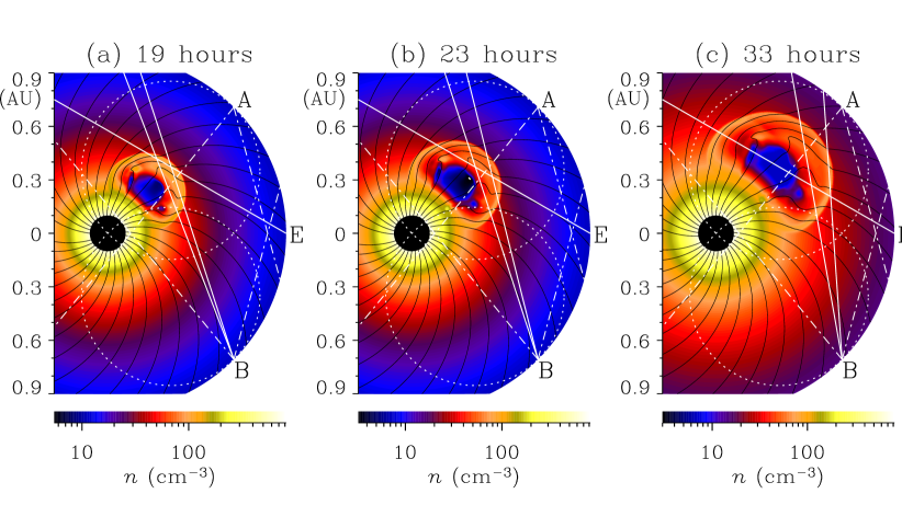
Figure 1: Density distribution $n$ in the ecliptic plane for the propagation of an interplanetary shock at (a) 19, (b) 23, and (c) 33 hours, following its initiation, with the interplanetary magnetic-field lines shown as solid black lines. The synthetic STEREO HI-A (HI-B) is at point ‘A’ (‘B’), with its Thomson-scattering sphere marked by a white dotted circle, and field of view marked by two dash-dotted lines. Note that the synthetic STEREO A and B spacecraft are located at $45^{\circ}$ in the longitude west and east from the Earth at point ‘E’, respectively. One solid line from the point ‘E’ denotes an IPS ray-path at the Earth with its elongation of $30^{\circ}$. Two solid lines from the point ‘B’ represent the elongation boundaries of relative-brightness enhancement $(I-I_{0})/I_{0}\geq 0.4$ in Figure 3.

Figure 4: The density $n$ (a) and speed $v_{\mbox{\tiny drift}}$ (b) profiles along an IPS ray-path for the background solar wind. Here, $v_{\mbox{\tiny drift}}$ refers to the speed component perpendicular to the IPS ray-path. Below are (c) the Auto-Correlation Function (ACF) and (d) the Cross-Correlation Function (CCF) from the IPS observations. The baseline between the two radio antennas is 2000 km, aligned with the solar wind outflow.

Figure 5: The density $n$ (a, e, i) and speed $v_{\mbox{\tiny drift}}$ (b, f, j) profiles along an IPS ray-path for a shock propagation. Below are (c, g, k) the Auto-Correlation Function (ACF) and (d, h, l) the Cross-Correlation Function (CCF) from the IPS observations. From the left to right, the three columns refer to three snapshots at 19, 23, and 33 hours, respectively, following the initiation of the event.

Figure 6: The profiles of the electron number $n\cdot r^{2}_{\mbox{\tiny HIB}}$ (a, d, g), radial bulk flow speed $v_{r}$ (b, e, h), and angular speed relative to the HI-B point $\Omega_{\mbox{\tiny HIB}}$ (c, f, i) along a specific ray-path $r_{\mbox{\tiny HIB}}$ at the elongation of $26^{\circ}$ at 19 hours, $30^{\circ}$ at 23 hours, and $38^{\circ}$ at 33 hours, viewed by the synthetic STEREO HI-B.

Figure 7: The time-dependent variances of (a) the radial aphelion $r$ and (b) the propagation speed $v_{\mbox{\tiny shock}}$ of a shock, as well as its manifestation in (c) the elongation of HI-B’s field of view, shown as black solid lines. In panel (b), the bulk flow speed $v_{r}$ and the fast magnetosonic speed $v_{r}+c_{f}$ just downstream of the shock front are plotted as a dashed line and a dash-dotted line respectively. As a specific plasma parcel on the shock front is firstly detected as an IPS irregularity source at 19 hours, its later appearances in the radial distance from the Sun (a dashed line in panel a) and the elongation from the HI (a dashed line in panel c) could be estimated from the IPS observation at 19 hours together with two assumptions of radial direction and constant flow speed for the shock propagation.

Figure 8: The infrastructure of a multi-scale numerical model directly linking interplanetary dynamics to corresponding observational signatures from white-light imaging and IPS. As a response to solar outputs, the macro-scale properties of electron number density $n$, bulk-flow speed $\mathbf{V}$, magnetic field $\mathbf{B}$, and temperature $T$ in interplanetary space are firstly modelled from an MHD simulation. These macro-scale profiles along any ray-path can then generate synthetic white-light image and IPS data, using Thomson-scattering and radio-scattering theories respectively.

References

- Armstrong et al. (1990) Armstrong, J. W., Coles, W. A., Rickett, B. J., Kojima, M., 1990. Observations of field-aligned density fluctuations in the inner solar wind. Astrophys. J. 358, 685–692.
- Bisi (2006) Bisi, M. M., 2006. Interplanetary scintillation studies of the large-scale structure of the solar wind. Ph.D. Thesis, Aberystwyth University, Wales, UK.
- Bisi et al. (2010) Bisi, M. M., Fallows, R. A., Breen, A. R., O’Neill, I. J., 2010. Interplanetary scintillation observations of stream interaction regions in the solar wind. Solar Phys. 261, 149–172.
- Bisi et al. (2008) Bisi, M. M., Jackson, B. V., Hick, P. P., Buffington, A., Odstrcil, D., Clover, J. M., 2008. Three-dimensional reconstructions of the early November 2004 Coordinated Data Analysis Workshop geomagnetic storms: Analyses of STELab IPS speed and SMEI density data. J. Geophys. Res. 113 (52), A00A11.
- Breen et al. (2008) Breen, A. R., Fallows, R. A., Bisi, M. M., Jones, R. A., Jackson, B. V., Kojima, M., Dorrian, G. D., Middleton, H. R., Thomasson, P., Wannberg, G., 2008. The solar eruption of 2005 May 13 and its effects: Long-baseline interplanetary scintillation observations of the Earth-directed coronal mass ejection. Astrophys. J. 683, L79–L82.
- Burlaga et al. (1987) Burlaga, L. F., Behannon, K. W., Klein, L. W., 1987. Compound streams, magnetic clouds, and major geomagnetic storms. J. Geophys. Res. 92 (A6), 5725–5734.
- Burlaga et al. (2002) Burlaga, L. F., Plunkett, S. P., Cyr, O. C. S., 2002. Successive CMEs and complex ejecta. J. Geophys. Res. 107.
- Colella and Woodward (1984) Colella, P., Woodward, P. R., 1984. The piecewise parabolic method (PPM) for gas-dynamical simulations. J. Comput. Phys. 54, 174–201.
- Coles and Harmon (1989) Coles, W. A., Harmon, J. K., 1989. Propagation observations of the solar wind near the Sun. Astrophys. J. 337, 1023–1034.
- Dal Lago et al. (2006) Dal Lago, A., Gonzalez, W. D., Balmaceda, L. A., Vieira, L. E. A., Echer, E., Guarnieri, F. L., Santos, J., da Silva, M. R., de Lucas, A., de Gonzalez, A. L. C., Schwenn, R., Schuch, N. J., 2006. The 17-22 October (1999) solar-interplanetary-geomagnetic event: Very intense geomagnetic storm associated with a pressure balance between interplanetary coronal mass ejection and a high-speed stream. J. Geophys. Res. 111, A07S14.
- Davies et al. (2009) Davies, J. A., Harrison, R. A., Rouillard, A. P., Jr., N. R. S., Perry, C. H., Bewsher, D., Davis, C. J., Eyles, C. J., Crothers, S. R., Brown, D. S., 2009. A synoptic view of solar transient evolution in the inner heliosphere using the Heliospheric Imagers on STEREO. Geophys. Res. Lett. 36, L02102.
- Davis et al. (2009) Davis, C. J., Davies, J. A., Lockwood, M., Rouillard, A. P., Eyles, C. J., Harrison, R. A., 2009. Sterescopic imaging of an earth-impacting solar coronal mass ejection: A major milestone for the STEREO mission. Geophys. Res. Lett. 36, L08102.
- Dorrian et al. (2008) Dorrian, G. D., Breen, A. R., Brown, D. S., Davies, J. A., Fallows, R. A., Rouillard, A. P., 2008. Simultaneous interplanetary scintillation and Heliospheric Imager observations of a coronal mass ejection. Geophys. Res. Lett. 35, L24104.
- Eyles et al. (2009) Eyles, C. J., Harrison, R. A., Davis, C. J., Waltham, N. R., Shaughnessy, B. M., Mapson-Menard, H. C. A., Bewsher, D., Crothers, S. R., Davies, J. A., Simnett, G. M., Howard, R. A., Moses, J. D., Newmark, J. S., Socker, D. G., Halain, J.-P., Defise, J.-M., Mazy, E., Rochus, P., 2009. The Heliospheric Imagers onboard the STEREO mission. Solar Phys. 254, 387–445.
- Fallows (2001) Fallows, R. A., 2001. Studies of the solar wind through a solar cycle. Ph.D. Thesis, Aberystwyth University, Wales, UK.
- Fallows et al. (2006) Fallows, R. A., Breen, A. R., Bisi, M. M., Jones, R. A., Wannberg, G., 2006. Dual-frequency interplanetary scintillation observations of the solar wind. Geophys. Res. Lett. 33 (11), L11106.
- Grall et al. (1997) Grall, R. R., Coles, W. A., Spangler, S. R., Sakurai, T., Harmon, J. K., 1997. Observations of field-aligned density microstructure near the sun. J. Geophys. Res. 102 (A1), 263–274.
- Hewish et al. (1964) Hewish, A., Scott, P. F., Willis, D., 1964. Interplanetary scintillation of small diameter radio sources. Nature 203, 1214.
- Houminer and Hewish (1972) Houminer, Z., Hewish, A., 1972. Long-lived sectors of enhanced density irregularities in the solar wind. Planetary and Space Science 20 (10), 1703–1716.
- Howard et al. (2008) Howard, R. A., Moses, J. D., Vourlidas, A., Newmark, J. S., Socker, D. G., Plunkett, S. P., Korendyke, C. M., Cook, J. W., Hurley, A., Davila, J. M., Thompson, W. T., St Cyr, O. C., Mentzell, E., Mehalick, K., Lemen, J. R., Wuelser, J. P., Duncan, D. W., Tarbell, T. D., Wolfson, C. J., Moore, A., Harrison, R. A., Waltham, N. R., Lang, J., Davis, C. J., Eyles, C. J., Mapson-Menard, H., Simnett, G. M., Halain, J. P., Defise, J. M., Mazy, E., Rochus, P., Mercier, R., Ravet, M. F., Delmotte, F., Auchere, F., Delaboudiniere, J. P., Bothmer, V., Deutsch, W., Wang, D., Rich, N., Cooper, S., Stephens, V., Maahs, G., Baugh, R., McMullin, D., Carter, T., 2008. Sun Earth Connection Coronal and Heliospheric Investigation (SECCHI). Space Sci. Review 136, 67–115.
- Howard and Tappin (2009) Howard, T. A., Tappin, S. J., 2009. Interplanetary coronal mass ejections observed in the heliosphere: 1. Review of theory. Space Sci. Review 147, 31–54.
- Hu (1998) Hu, Y. Q., 1998. Asymmetric propagation of flare-generated shocks in the heliospheric equatorial plane. J. Geophys. Res. 103 (A7), 14,631–14,642.
- Hu et al. (2007) Hu, Y. Q., Guo, X. C., Wang, C., 2007. On the ionospheric and reconnection potentials of the earth: Results from global MHD simulations. J. Geophys. Res. 112, A07215.
- Jackson et al. (2003) Jackson, B. V., Hick, P. P., Buffington, A., Kojima, M., Tokumaru, M., Fujiki, K., Ohmi, T., Yamashita, M., 2003. Time-dependent tomography of hemispheric features using interplanetary scintillation (IPS) remote-sensing observations. In: Velli, M., Bruno, R., Malara, F., Bucci, B. (Eds.), Solar Wind Ten. Vol. AIP Conf. of 679. p. 75.
- Jeffrey and Taniuti (1964) Jeffrey, A., Taniuti, T., 1964. Non-Linear Wave Propagation with Application to Physics and Magnetohydrodynamics. Academic Press, New York.
- Kaiser (2008) Kaiser, M. L.; Kucera, T. A. D. J. M. S. C. O. C. G. M. C. E., 2008. The STEREO mission: An introduction. Space Sci. Review 136, 5–16.
- Klinglesmith (1997) Klinglesmith, M., 1997. The polar solar wind from 2.5 to 40 solar radii: Results of intensity scintillation measurements. Ph.D. Thesis, University of California, San Diego, USA.
- Lepping et al. (1997) Lepping, R. P., Burlaga, L. F., Szabo, A., Ogilvie, K. W., Mish, W. H., Vassiliadis, D., Lazarus, A. J., Steinberg, J. T., Farrugia, C. J., Janoo, L., Mariani, F., 1997. The Wind magnetic cloud and events of October 18-20, 1995: Interplanetary properties and as triggers for geomagnetic activity. J. Geophys. Res. 102 (A7), 14,049–14,063.
- Lugaz et al. (2009) Lugaz, N., Vourlidas, A., Roussev, I. I., Morgan, H., 2009. Solar-terrestrial simulation in the STEREO era: The 24-25 January 2007 eruptions. Solar Phys. 256, 269–284.
- Massey (1998) Massey, W., 1998. Measuring intensity scintillations at the Very Long Baseline Array (VLBA) to probe the solar wind near the Sun. Master Thesis, University of California, San Diego, USA.
- McComas et al. (2000) McComas, D. J., Barraclough, B. L., Funsten, H. O., Gosling, J. T., Santiago-Munoz, E., Skoug, R. M., Goldstein, B. E., Neugebauer, M., Riley, P., Balogh, A., 2000. Solar wind observations over Ulysses’ first full polar orbit. J. Geophys. Res. 105, 10,419–10,434.
- Odstrcil and Pizzo (2009) Odstrcil, D., Pizzo, V. J., 2009. Numerical heliospheric simulations as assisting tool for interpretation of observations by STEREO Heliospheric Imagers. Solar Phys. 259, 297–309.
- Rouillard et al. (2008) Rouillard, A. P., Davies, J. A., Forsyth, R. J., Rees, A., Davis, C. J., Harrison, R. A., Lockwood, M., Bewsher, D., Crothers, S. R., Eyles, C. J., Hapgood, M., Perry, C. H., 2008. First imaging of corotating interaction regions using the STEREO spacecraft. Geophys. Res. Lett. 35, L10110.
- Rouillard et al. (2009) Rouillard, A. P., Savani, N. P., Davies, J. A., Lavraud, B., Forsyth, R. J., Morley, S. K., Opitz, A., Sheeley, N. R., Burlaga, L. F., Sauvaud, J.-A., Simunac, K. D. C., Luhmann, J. G., Galvin, A. B., Crothers, S. R., Davis, C. J., Harrison, R. A., Lockwood, M., Eyles, C. J., Bewsher, D., Brown, D. S., 2009. A multispacecraft analysis of a small-scale transient entrained by solar wind streams. Solar Phys. 256, 307–326.
- Salpeter (1967) Salpeter, E. E., 1967. Interplanetary scintillations: I. Theory. Astrophys. J. 147, 433.
- Sheeley et al. (2008) Sheeley, N. R., Herbst, A. D., Palatchi, C. A., Wang, Y.-M., Howard, R. A., Moses, J. D., Vourlidas, A., Newmark, J. S., Socker, D. G., Plunkett, S. P., Korendyke, C. M., Burlaga, L. F., Davila, J. M., Thompson, W. T., St Cyr, O. C., Harrison, R. A., Davis, C. J., Eyles, C. J., Halain, J. P., Wang, D., Rich, N. B., Battams, K., Esfandiari, E., Stenborg, G., 2008. SECCHI observations of the Sun’s garden-hose density spiral. Astrophys. J. 674, 109.
- Tatarski et al. (1993) Tatarski, V., Ishimaru, A., Zavorotny, V., 1993. Wave propagation in a random medium (Scintillation). SPIE Press, Bellingham.
- Vourlidas and Howard (2006) Vourlidas, A., Howard, R. A., 2006. The proper treatment of coronal mass ejection brightness: A new methodology and implications for observations. Astrophys. J. 642, 1216–1221.
- Vourlidas et al. (2000) Vourlidas, A., Subramanian, P., Dere, K. P., Howard, R. A., 2000. Large-angle spectrometric coronagraph measurements of the energetics of coronal mass ejections. Astrophys. J. 534, 456–467.
- Webb et al. (2009) Webb, D. F., Howard, T. A., Fry, C. D., Kuchar, T. A., Odstrcil, D., Jackson, B. V., Bisi, M. M., Harrison, R. A., Morrill, J. S., Howard, R. A., Johnston, J. C., 2009. Study of CME propagation in the inner heliosphere: SOHO LASCO, SMEI and STEREO HI observations of the January 2007 events. Solar Phys. 256, 239–267.
- Wei et al. (2006) Wei, F. S., Feng, X. S., Yang, F., Zhong, D., 2006. A new non-pressure-balanced structure in interplanetary space: Boundary layers of magnetic clouds. J. Geophys. Res. 111.
- Xiong et al. (2009) Xiong, M., Zheng, H. N., Wang, S., 2009. Magnetohydrodynamic simulation of the interaction between two interplanetary magnetic clouds and its consequent geoeffectiveness: 2. Oblique collision. J. Geophys. Res. 114, A11101.
- Xiong et al. (2006a) Xiong, M., Zheng, H. N., Wang, Y. M., Wang, S., 2006a. Magnetohydrodynamic simulation of the interaction between interplanetary strong shock and magnetic cloud and its consequent geoeffectiveness. J. Geophys. Res. 111, A08105.
- Xiong et al. (2006b) Xiong, M., Zheng, H. N., Wang, Y. M., Wang, S., 2006b. Magnetohydrodynamic simulation of the interaction between interplanetary strong shock and magnetic cloud and its consequent geoeffectiveness: 2. Oblique collision. J. Geophys. Res. 111, A11102.
- Xiong et al. (2007) Xiong, M., Zheng, H. N., Wu, S. T., Wang, Y. M., Wang, S., 2007. Magnetohydrodynamic simulation of the interaction between two interplanetary magnetic clouds and its consequent geoeffectiveness. J. Geophys. Res. 112, A11103.