Abstract

We introduce and analyze a system of two coupled partial differential equations with external noise. The equations are constructed to model transitions of monovalent metallic nanowires with non-axisymmetric intermediate or end states, but also have more general applicability. They provide a rare example of a system for which an exact solution of nonuniform stationary states can be found. We find a transition in activation behavior as the interval length on which the fields are defined is varied. We discuss several applications to physical problems.

Lan Gong1 and D. L. Stein1,2

lan.gong@nyu.edu   daniel.stein@nyu.edu

1Department of Physics, New York University, New York, NY 10003

2Courant Institute of Mathematical Sciences, New York University, New York, NY 10003

1 Introduction

A locally stable system subject to random perturbations will eventually be driven from its basin of attraction by a sufficiently large fluctuation. The case of weak noise is particularly important, and often arises in stochastic modeling of physical and non-physical systems [1, 2, 3, 4, 5, 6, 7, 8, 9, 10]. Noisy systems in which spatial variation of some intrinsic property cannot be ignored arise in numerous contexts and are therefore of particular interest [11]. Examples include micromagnetic domain reversal [12, 13], pattern nucleation [14, 15, 16], transitions in hydrogen-bonded ferroelectrics [17], dislocation motion across Peierls barriers [18], and structural transitions in metallic nanowires [19, 20].

Noise-induced escape can occur through either classical or quantum processes. In classical systems, where escape involves activation over a barrier, the source of the noise is often, but not always, thermal in origin. The field-theoretic techniques for computing escape rates in these systems were developed by Langer [21, 22], who considered the homogeneous nucleation of one phase inside another. In a quantum system at sufficiently low temperature, escape occurs by tunneling through a barrier; although the process is physically different, the mathematical formalism is similar to that of the classical case. The basic theory here was worked out by Coleman and Callan [23, 24, 25] in the context of quantum tunneling out of a “false vacuum”. A review of the basic approach in both cases can be found in [9, 26].

All of these consider the case of an infinite system. The equivalent problem on a finite spatial domain was first studied by Faris and Jona-Lasinio [27, 28], who developed a large deviation theory of the leading-order exponential term in activated barrier crossing for the special case of Dirichlet boundary conditions. General techniques for computing the activation prefactor were developed by Forman [29] and McKane and Tarlie [30]. In general, computation of the subdominant behavior of activated processes (the rate prefactor, the distribution of exit points, and related quantities) requires knowledge of the transition state, which describes the system configuration at the col, or barrier ‘top’. When this state is spatially nonuniform, as typically occurs at all but the shortest system sizes, it can typically only be found as the solution of a nonlinear differential equation. This usually requires numerical techniques; nontrivial problems where analytical solutions can be found are rare.

When spatial variation can be ignored, the dynamical evolution of a noisy system can be modelled using a stochastic ordinary differential equation; when it can’t, a stochastic partial differential equation is required. This can and does lead to new phenomena; one of these is a phase transition in activation behavior as some system parameter is varied. In classical systems confined to a finite domain this transition can occur as system size (or some other parameter such as external magnetic field in a magnetic system) changes [31, 32]; in quantum systems, an analogous quantum tunneling$\leftrightarrow$classical activation transition occurs as temperature increases [33, 34, 35, 36, 37, 38]. This phase transition has a profound effect on activation behavior, and can have physically observable consequences [20].

Most of the cases studied to date require only a single classical field to describe the spatial variation of the system. However, situations can arise in which two (or more) fields are necessary to model the system. These have received little attention to date; one notable exception is the analysis of Tarlie et al. [39] which studied phase slippage in conventional superconducting rings. In this case, the spatial and gauge symmetries imposed by the physics allowed an exact solution of the transition state to be found. More generally, such symmetries are absent, and it is of interest to find more general systems in which exact solutions can similarly be found.

In this paper we propose and analyze one such model that may have wide applicability; it can be regarded as a generalization of the system studied in [39]. The model was motivated by the growing body of research on metallic wires of several nanometer diameters and lengths of the order of tens of nanometers [40, 41, 42, 43, 44, 45, 46, 47], which represent the ultimate size limit of conductors and are of interest from the point of view of both fundamental physics and technological applications. However, as we discuss in the conclusions, the model and its solutions may apply as well to other problems of interest. We therefore confine our discussion in this paper to the mathematical features of the model and its solution. Its specific application to nanowires — which will necessarily involve additional modelling — will appear elsewhere [48].

2 Monovalent Metalic Nanowires

Nevertheless, to set the stage for introduction of the model, we briefly discuss the problem of stability and lifetimes of nanowires composed of metals from either the alkali or the noble metal groups. Because the stresses induced by surface tension at the nanometer lengthscale exceeds the Young’s modulus, such wires are subject to deformation under plastic flow [49]. A purely classical wire would therefore be subject to breakup due to the Rayleigh instability, and this in fact has been observed for copper nanowires annealed between 400 and 600^∘C [50]. However, a nanowire is sufficiently small for quantum effects to also play a role, and indeed a quantum linear stability analysis [49, 51, 52, 53] showed that at discrete values of the radius, the Rayleigh instability is suppressed. These radii correspond to conductance “magic numbers” that agree with those observed in experiments [46, 54, 55].

The linear stability analysis, however, ignores thermal noise that can induce rare but large radius fluctuations leading to breakup. A self-consistent approach to determining lifetimes [56, 19], which modelled thermal fluctuations through a stochastic Ginzburg-Landau classical field theory, obtained quantitative estimates of alkali nanowire lifetimes, in good agreement with experimentally inferred values [46, 54, 55]. The theory restricted itself to perfectly cylindrical wires, so that a single classical field could be used to represent radius fluctuations along the length of the wire.

To test the assumption of axial symmetry along the cylinder axis, Urban et al. [57] performed a stability analysis of metal nanowires subject to non-axisymmetric perturbations. They were able to show that, at certain mean radii and aspect ratios, Jahn-Teller deformations breaking cylindrical symmetry can be energetically favorable, leading to stable nanowires with non-axisymmetric cross sections. They predicted that a typical mechanically controllable break junction experiment should observe roughly 3/4 cylindrical wires and 1/4 noncylindrical.

The mathematical problem can be understood as follows. Urban et al. [58] considered non-axisymmetric deformations in the wire cross-section of the form $\cos(m\phi)$, i.e., having $m$-fold symmetry. The radius function describing the surface of a wire of cross-sectional area $\pi\rho(z)^{2}$ at position $z$ along the wire length is then

$$R(\rho,\phi)=\rho(z)\Biggl{(}\sqrt{1-\sum_{m}\lambda_{m}(z)^{2}/2}+\sum_{m}\lambda_{m}(z)\cos[m(\phi-\phi_{m})]\Biggr{)}\,,$$ (1)

where the sums run over the positive integers and the deformation parameters $\lambda_{m}(z)$ that represent deviations from axial symmetry are considered small.

Urban et al. studied deformations with $m\leq 6$, but focused mostly on $m=2$, i.e., quadrupolar deformations. Deformations of order higher than $m=6$ cost more surface energy and are therefore less stable. $m=1$ corresponds to a simple translation. One can then consider only deviations from axisymmetry of the form shown in Fig. 1.

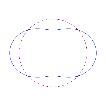
Figure 1: Solid line is the deformed cross section at $m=2$

Using a linear stability analysis (which again ignores large thermal fluctuations) they found several sequences of stable wires, some with considerable deviations from axial symmetry. Fig. 2 shows the phase diagram of linear stability in the configuration space of the two deformation parameters: the Sharvin conductance $G_{s}$ and the coefficient of the quadrupole deformation $\lambda_{2}$. The $x$-axis gives a measure of the average radius parameter $\rho$, which is related to the square root of the Sharvin conductance [59].

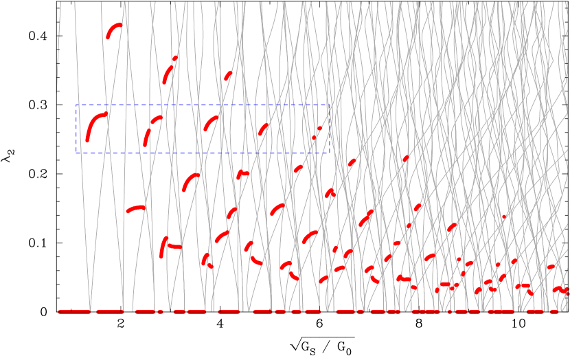
Figure 2: Linearly stable quadrupolar Na wires (thick lines) at low temperature, shown in the deformation configuration space $(\rho,\lambda_{2})$, where $\rho$ is related to the Sharvin conductance by $\sqrt{G_{s}/G_{0}}\approx k_{F}\rho/2$. The thin grey lines show the thresholds for the openings of new conductance channels. Thick lines along the $x$-axis ($\lambda_{2}=0$) denote regions of stability for purely cylindrical wires. (From Urban et al. [58].)

In order to construct a comprehensive theory of nanowire lifetimes, then, it is necessary to extend the theory developed in [56, 19] to non-axisymmetric wires. This requires, as noted earlier, a consideration of a classical stochastic Ginzburg-Landau field theory with two fields, with one representing variation of the radius along the longitudinal axis and the other the departure from axisymmetry.

3 The Model

From the preceding discussion, it is evident that a minimal description of fluctuations in a non-axisymmetric wire requires two fields: the first, which we denote $\phi_{1}(z)$, is related to $\rho(z)$ and characterizes radius fluctuations about some fixed average $\rho_{0}$; the second, which we denote $\phi_{2}(z)$, is simply $\lambda_{2}(z)$ and characterizes deviations from axisymmetry. A wire with a perfectly cylindrical cross-section everywhere would have $\phi_{2}(z)=0$.

Although developing a theory of fluctuations of non-axisymmetric wires provides a physical motivation for studying classical Ginzburg-Landau theories with two fields, we are also interested in the general problem of such field theories. In this paper, we therefore construct and study a model which applies not only to some (but not all) transitions among non-axisymmetric wires, but also to other problems as well. This will be discussed further in Sect. 6.

We therefore consider on $[-L/2,L/2]$ two classical fields $\phi_{1}(z,t)$, $\phi_{2}(z,t)$ subject to the potential

$$U(\phi_{1},\phi_{2})=-\frac{\mu_{1}}{2}\phi_{1}^{2}+\frac{1}{4}\phi_{1}^{4}-\frac{\mu_{2}}{2}\phi_{2}^{2}+\frac{1}{4}\phi_{2}^{4}+\frac{1}{2}\phi_{1}^{2}\phi_{2}^{2}$$ (2)

where $\mu_{1}$ and $\mu_{2}$ are arbitrary positive constants such that $\mu_{1}\neq\mu_{2}$, breaking rotational symmetry between the two fields. A contour map of the potential is given in Fig. 3.

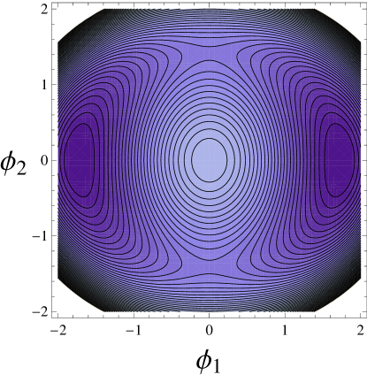
Figure 3: Equipotential contours in $U(\phi_{1},\phi_{2})$ for the fields $\phi_{1}$ and $\phi_{2}$ when $\mu_{1}=3$ and $\mu_{2}=2$.

If the two fields are subject to the potential (2), have bending coefficients of $\kappa_{1}$ and $\kappa_{2}$ respectively (in the nanowire case these can be related to surface tension), and are subject to additive spatiotemporal white noise, then their time evolution is governed by the pair of coupled stochastic partial differential equations

$$\dot{\phi_{1}}=\kappa_{1}\phi_{1}^{\prime\prime}+\mu_{1}\phi_{1}-\phi_{1}^{3}-\phi_{1}\phi_{2}^{2}+\epsilon^{1/2}\xi_{1}(z,t)$$

$$\dot{\phi_{2}}=\kappa_{2}\phi_{2}^{\prime\prime}+\mu_{2}\phi_{2}-\phi_{2}^{3}-\phi_{1}^{2}\phi_{2}+\epsilon^{1/2}\xi_{2}(z,t)\,,$$ (3)

where $<\xi_{i}(z_{1},t_{1})\xi_{j}(z_{2},t_{2})>=\delta(z_{1}-z_{2})\delta(t_{1}-t_{2})\delta_{ij},~{}i,j=1,2$. We will make the simplifying assumption here that $\kappa_{1}=\kappa_{2}=1$. When $\mu_{1}=\mu_{2}$, it can be shown that the above equations are equivalent to those studied by Tarlie et al. [39] to model fluctuations in superconducting rings. The breaking of symmetry between the fields leads to an entirely different behavior from what was found for that case.

The zero-noise dynamics satisfy $\dot{\phi_{i}}=-\delta H/\delta\phi_{i}$, with the energy functional

$$H=\int_{-L/2}^{L/2}\!(\frac{1}{2}(\phi_{1}^{\prime}(z))^{2}+\frac{1}{2}(\phi_{2}^{\prime}(z))^{2}+U(\phi_{1},\phi_{2}))\,dz\,.$$ (4)

The metastable and saddle, or transition, states are time-independent solutions of the zero-noise equations, [9] satisfying the Euler-Lagrange equations

$$\phi_{1}^{\prime\prime}=-\mu_{1}\phi_{1}+\phi_{1}^{3}+\phi_{1}\phi_{2}^{2}$$

$$\phi_{2}^{\prime\prime}=-\mu_{2}\phi_{2}+\phi_{2}^{3}+\phi_{1}^{2}\phi_{2}$$ (5)

At nonzero temperature, thermal fluctuations can drive the system from one metastable state to another. Such a transition proceeds via a pathway of states that first goes uphill in energy from the starting configuration, passes through (or close to) a saddle configuration, and then proceeds downhill towards the nearest metastable state. The activation rate is given in the $T\to 0$ limit by the Kramers formula [9]

$$\Gamma\sim\Gamma_{0}\exp(-\Delta E/T)\,.$$ (6)

Here $\Delta E$ is the activation barrier, the difference in energy between the saddle and the starting metastable configuration, and $\Gamma_{0}$ is the rate prefactor.

The quantities $\Delta E$ and $\Gamma_{0}$ depend on the details of the potential (2), on the interval length $L$ on which the fields are defined, and on the choice of boundary conditions at the endpoints $z=-L/2$ and $z=L/2$. It was shown in [60] that Neumann boundary conditions are appropriate for the nanowire problem, and we will use them here. However, the theory is easily extended to other types of boundary conditions [61], although for periodic boundary conditions care must be taken to extract the zero mode when performing prefactor computations [30].

From here on, we choose without loss in generality $\mu_{1}>\mu_{2}$. In this case there are two uniform metastable states $\phi_{1s}=\pm\sqrt{\mu_{1}},\phi_{2s}=0$ and two uniform transition states $\phi_{1u}=0,\phi_{2u}=\pm\sqrt{\mu_{2}}$, as can be seen in Fig. 3. In the following section, we will see that the uniform transition states are true saddles, and therefore relevant for escape, only when $L<L_{c}=\frac{\pi}{\sqrt{\mu_{1}-\mu_{2}}}$. At $L_{c}$, a transition occurs, and above it the transition states are nonuniform.

4 The Transition State

We have found analytical solutions to Eqs. (3) that describe nonuniform saddle configurations (hereafter referred to as “instantons”, in keeping with the usual practice). For general $\mu_{1}>\mu_{2}$ they are:

$$\phi^{\rm inst}_{1,m}(z)=\pm\sqrt{m}\sqrt{(2\mu_{1}-\mu_{2})-m(\mu_{1}-\mu_{2})}{\rm sn}(\sqrt{\mu_{1}-\mu_{2}}\,z|m)$$ (7)

$$\phi^{\rm inst}_{2,m}(z)=\pm\sqrt{\mu_{2}-m(\mu_{1}-\mu_{2})}{\rm dn}(\sqrt{\mu_{1}-\mu_{2}}\,z|m)$$ (8)

where ${\rm sn}(.|m)$and ${\rm dn}(.|m)$ are the Jacobi elliptic functions with parameter $m$, whose periods are $4K(m)$ and $2K(m)$ respectively, with $K(m)$ the complete elliptic integral of the first kind [62]. Imposing Neumann boundary conditions yields a relation between $L$ and $m$:

$$L=\frac{2K(m)}{\sqrt{\mu_{1}-\mu_{2}}}$$ (9)

The instanton states for $\mu_{1}=3$, $\mu_{2}=2$ and intermediate $m$ are shown in Fig. 4.

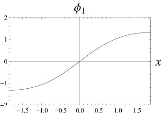
(a) $\phi^{\rm inst}_{1,m}(z)$

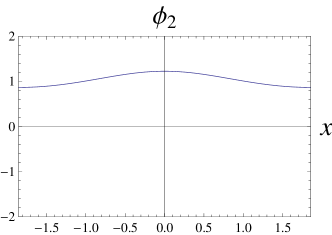
(b) $\phi^{\rm inst}_{2,m}(z)$

Figure 4: The instanton states $\phi^{\rm inst}_{i,m}$ for $\mu_{1}=3$, $\mu_{2}=2$, and $m=1/2$.

As $m\to 0$, $L$ approaches its minimum length $L_{c}=\frac{\pi}{\sqrt{\mu_{1}-\mu_{2}}}$. In this limit, $\phi^{\rm inst}_{1,0}=0$, $\phi^{\rm inst}_{2,0}=\pm\sqrt{\mu_{2}}$, and the instantons reduce to the spatially uniform saddle states. As $m\to 1^{-}$, $L\to\infty$, and the instanton states become

$$\phi^{\rm inst}_{1,1}=\pm\sqrt{\mu_{1}}\,\tanh(\sqrt{\mu_{1}-\mu_{2}}\,z)$$ (10)

$$\phi^{\rm inst}_{2,1}=\pm\sqrt{2\mu_{2}-\mu_{1}}\,{\rm sech}(\sqrt{\mu_{1}-\mu_{2}}\,z)$$ (11)

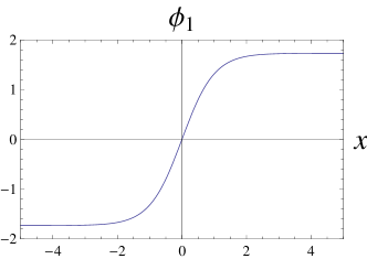
(a) $\phi^{\rm inst}_{1,m}(z)$

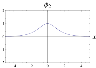
(b) $\phi^{\rm inst}_{2,m}(z)$

Figure 5: The instanton states $\phi^{\rm inst}_{i,m}$ for infinite length as $m\to 1^{-}$ for $\mu_{1}=3$, $\mu_{2}=2$.

In the nanowire case, there is a nice geometric interpretation of this particular version of the escape process, which will be discussed in Sect. 6.

At low temperatures, the leading order asymptotic dependence ($\Delta E$ in the Kramers formula) of the escape rate can be computed as the difference in energy between the saddle and stable configurations, and is plotted in Fig. 6.

Figure 6: The activation barrier $\Delta E$ for Neumann boundary condition (solid line) at $\mu_{1}=3,\mu_{2}=2$. The dashed line indicates the crossover from the uniform transition states to the instanton transition states at $L_{c}$. The dots represent the numerical results of $\Delta E$ beyond $L_{c}$.

As $L\to\infty$, $\Delta E$ approaches $\frac{2}{3}\sqrt{\mu_{1}-\mu_{2}}(\mu_{1}+2\mu_{2})$. This is simply the energy of the domain walls of Figs. 5a, 5b.

5 Rate Prefactor

For an overdamped system driven by white noise, the rate prefactor $\Gamma_{0}$ can be derived in principle [9], although this is often difficult in practice. The usual procedure is to consider small perturbations $\eta_{1}$, $\eta_{2}$ about the metastable state: $\phi_{1}=\phi_{1,s}+\eta_{1}$ and $\phi_{2}=\phi_{2,s}+\eta_{2}$. Then to leading order $\dot{\vec{\eta}}=-{\bf\Lambda}_{s}{\vec{\eta}}$, ${\vec{\eta}}=(\eta_{1},\eta_{2})$, where ${\bf\Lambda}_{s}$ is the linearized zero-noise dynamical operator at $\phi_{1,s}$, $\phi_{2,s}$. Similarly, ${\bf\Lambda}_{u}$ is the linearized zero-noise dynamical operator at the transition state $\phi_{1,u}$,$\phi_{2,u}$. Then [9]

$$\Gamma_{0}=\frac{1}{\pi}\sqrt{\left|\frac{\det\,{\bf\Lambda}_{s}}{\det\,{\bf\Lambda}_{u}}\right|}|\lambda_{u,1}|$$ (12)

where $\lambda_{u,1}$ is the single negative eigenvalue of ${\bf\Lambda}_{u}$, corresponding to the direction along which the optimal escape trajectory approaches the transition state. Here Eq. (12) differs from the usual formula for $\Gamma_{0}$ [2, 9] by a factor of 2 in the denominator because we have two saddle points distributed symmetrically between the metastable states (see Fig. 3) such that the transition can take place via either. In the next two sections, we consider two interval length regimes, each with different saddle configurations.

5.1 $L<L_{c}$

In this regime, both the metastable and transition states are spatially uniform, allowing for a straightforward computation of $\Gamma_{0}$. Assume the system begins at the metastable state $(-\sqrt{\mu_{1}},0)$, passes through the transition state $(0,\sqrt{\mu_{2}})$, and finishes at $(\sqrt{\mu_{1}},0)$. Linearization around the metastable state gives

$$\frac{d}{dt}\begin{pmatrix}\eta_{1}\\ \eta_{2}\end{pmatrix}=-{\bf\Lambda}_{s}\begin{pmatrix}\eta_{1}\\ \eta_{2}\end{pmatrix}=-\begin{pmatrix}-\partial_{z}^{2}+2\mu_{1}&0\\ 0&-\partial_{z}^{2}+(\mu_{1}-\mu_{2})\end{pmatrix}\begin{pmatrix}\eta_{1}\\ \eta_{2}\end{pmatrix}$$ (13)

and around the transition state

$$\frac{d}{dt}\begin{pmatrix}\eta_{1}\\ \eta_{2}\end{pmatrix}=-{\bf\Lambda}_{u}\begin{pmatrix}\eta_{1}\\ \eta_{2}\end{pmatrix}=-\begin{pmatrix}-\partial_{z}^{2}-(\mu_{1}-\mu_{2})&0\\ 0&-\partial_{z}^{2}+2\mu_{2}\end{pmatrix}\begin{pmatrix}\eta_{1}\\ \eta_{2}\end{pmatrix}\,.$$ (14)

The spectrum corresponding to ${\bf\Lambda}_{s}$ is

$$\lambda_{n}^{s}=\left\{\begin{array}[]{l l}\frac{\pi^{2}n_{1}^{2}}{L^{2}}+2\mu_{1}&\quad n_{1}=0,1,2...\\ \\ \frac{\pi^{2}n_{2}^{2}}{L^{2}}+(\mu_{1}-\mu_{2})&\quad n_{2}=0,1,2...\\ \end{array}\right.$$

and that corresponding to ${\bf\Lambda}_{u}$ is

$$\lambda_{n}^{u}=\left\{\begin{array}[]{l l}\frac{\pi^{2}n_{1}^{2}}{L^{2}}-(\mu_{1}-\mu_{2})&\quad n_{1}=0,1,2...\\ \\ \frac{\pi^{2}n_{2}^{2}}{L^{2}}+2\mu_{2}&\quad n_{2}=0,1,2...\\ \end{array}\right.$$

When $L<L_{c}$, all the eigenvalues of ${\bf\Lambda}_{u}$ are positive, except for $\lambda_{n_{1}=0}^{u}=-(\mu_{1}-\mu_{2})$, indicating that this is indeed a saddle configuration. The eigenfunction corresponding to $\lambda_{n_{1}=0}^{u}$, which is spatially uniform, is the direction in configuration space along which the optimal escape path approaches $(0,\sqrt{\mu_{2}})$. The fact that the lowest positive eigenvalue $\lambda_{n_{1}=1}^{u}\to 0$ as $L\to L_{c}^{-}$ indicates a transition in the escape dynamics at $L_{c}$.

This in turn affects the rate prefactor, which for $L<L_{c}$ is

$$\begin{split}\Gamma_{0}=&\frac{1}{\pi}\sqrt{\left|\frac{\prod_{n_{1}=0}^{\infty}\left(2\mu_{1}+\frac{\pi^{2}n_{1}^{2}}{L^{2}}\right)}{\prod_{n_{2}=0}^{\infty}\left(2\mu_{2}+\frac{\pi^{2}n_{2}^{2}}{L^{2}}\right)}\right|}\sqrt{\left|\frac{\prod_{n_{2}=0}^{\infty}\left((\mu_{1}-\mu_{2})+\frac{\pi^{2}n_{2}^{2}}{L^{2}}\right)}{\prod_{n_{1}=0}^{\infty}\left(-(\mu_{1}-\mu_{2})+\frac{\pi^{2}n_{1}^{2}}{L^{2}}\right)}\right|}|-(\mu_{1}-\mu_{2})|\\ =&\frac{1}{\pi}\sqrt{\frac{\sqrt{\mu_{1}}}{\sqrt{\mu_{2}}}}\frac{\sqrt{\sinh(\sqrt{\mu_{1}-\mu_{2}}L)}}{\sqrt{\sinh(\sqrt{2\mu_{2}}L)}}\frac{\sqrt{\sinh(\sqrt{2\mu_{1}}L)}}{\sqrt{|\sin(\sqrt{\mu_{1}-\mu_{2}}L)|}}(\mu_{1}-\mu_{2})\,.\end{split}$$ (15)

The prefactor diverges at $L_{c}=\frac{\pi}{\sqrt{\mu_{1}-\mu_{2}}}$. The divergence arises from the vanishing of $\lambda_{n_{1}=1}^{u}=\frac{\pi^{2}}{L^{2}}-(\mu_{1}-\mu_{2})$, indicating an appearance of a transverse soft mode in the fluctuations about the transition state.

5.2 $L>L_{c}$

When the transition is nonuniform, computation of the determinant ratio is less straightforward. Here the linearized operator ${\bf\Lambda}_{u}$ about the transition state is

$${\bf\Lambda}_{u}=\begin{pmatrix}-\partial_{z}^{2}-(\mu_{1}-3(\phi^{\rm inst}_{1,m})^{2}-(\phi^{\rm inst}_{2,m})^{2})&2\phi^{\rm inst}_{1,m}\phi^{\rm inst}_{2,m}\\ 2\phi^{\rm inst}_{1,m}\phi^{\rm inst}_{2,m}&-\partial_{z}^{2}-(\mu_{2}-3(\phi^{\rm inst}_{2,m})^{2}-(\phi^{\rm inst}_{1,m})^{2})\end{pmatrix}$$ (16)

and the linearized equations become a pair of second order coupled nonlinear differential equations.

In order to calculate $\det{\bf{\bf\Lambda}}_{s}/\det{\bf{\bf\Lambda}}_{u}$ we make use of a generalization, due to Forman [29], of the Gel’fand-Yaglom technique [63], suitable for differential operators in a $2\times 2$-matrix. The Forman method is readily extendible to higher dimensions [64], and its central result is that

$$\frac{\det{\bf\Lambda}_{s}}{\det{\bf\Lambda}_{u}}=\frac{\det[{\bf M}+{\bf NY}_{s}(L/2)]}{\det[{\bf M}+{\bf NY}_{u}(L/2)]}\,.$$ (17)

The $4\times 4$ matrices ${\bf Y}_{s}(z)$, ${\bf Y}_{u}(z)$ in (17) are “fundamental” matrices[65]. A fundamental matrix ${\bf Y}(z)$ has the property that, for any solution ${\vec{\eta}}(z)$ of the homogeneous equation ${\bf\Lambda}{\vec{\eta}}=0$,

$$\begin{pmatrix}\eta_{1}(z)\\ \eta_{2}(z)\\ \eta_{1}^{\prime}(z)\\ \eta_{2}^{\prime}(z)\end{pmatrix}={\bf Y}(z)\begin{pmatrix}\eta_{1}(-L/2)\\ \eta_{2}(-L/2)\\ \eta_{1}^{\prime}(-L/2)\\ \eta_{2}^{\prime}(-L/2)\,.\end{pmatrix}$$ (18)

The matrices ${\bf Y}_{s}(z)$, ${\bf Y}_{u}(z)$ are then defined to be fundamental matrices of the differential equations

$$\frac{d}{dz}\begin{pmatrix}\eta_{1}\\ \eta_{2}\\ \eta_{1}^{\prime}\\ \eta_{2}^{\prime}\end{pmatrix}=\begin{pmatrix}0&0&1&0\\ 0&0&0&1\\ 2\mu_{1}&0&0&0\\ 0&\mu_{1}-\mu_{2}&0&0\end{pmatrix}\begin{pmatrix}\eta_{1}\\ \eta_{2}\\ \eta_{1}^{\prime}\\ \eta_{2}^{\prime}\end{pmatrix}$$ (19)

$$\frac{d}{dz}\begin{pmatrix}\eta_{1}\\ \eta_{2}\\ \eta_{1}^{\prime}\\ \eta_{2}^{\prime}\end{pmatrix}=\begin{pmatrix}0&0&1&0\\ 0&0&0&1\\ -(\mu_{1}-3(\phi^{\rm inst}_{1,m})^{2}-(\phi^{\rm inst}_{2,m})^{2})&2\phi^{\rm inst}_{1,m}\phi^{\rm inst}_{2,m}&0&0\\ 2\phi^{\rm inst}_{1,m}\phi^{\rm inst}_{2,m}&-(\mu_{2}-3(\phi^{\rm inst}_{2,m})^{2}-(\phi^{\rm inst}_{1,m})^{2})&0&0\end{pmatrix}\begin{pmatrix}\eta_{1}\\ \eta_{2}\\ \eta_{1}^{\prime}\\ \eta_{2}^{\prime}\end{pmatrix}$$ (20)

which are just the equivalent first order versions of ${\bf\Lambda}_{s}$ and ${\bf\Lambda}_{u}$ (for $L>L_{c}$). The matrices ${\bf Y}_{s}(z)$, ${\bf Y}_{u}(z)$ will be discussed further below.

The $4\times 4$ matrices ${\bf M}$ and ${\bf N}$ encode the boundary conditions

$${\bf M}\,\begin{pmatrix}{\vec{\eta}}(-L/2)\\ {\vec{\eta}}\,^{\prime}(-L/2)\end{pmatrix}+{\bf N}\,\begin{pmatrix}{\vec{\eta}}(L/2)\\ {\vec{\eta}}\,^{\prime}(L/2)\end{pmatrix}=0\,.$$ (21)

For Neumann boundary conditions, $${\bf M} {\bf N}$$ and have the forms

$${\bf M}=\begin{pmatrix}0&0&1&0\\ 0&0&0&1\\ 0&0&0&0\\ 0&0&0&0\end{pmatrix}$$ (22)

and

$${\bf N}=\begin{pmatrix}0&0&0&0\\ 0&0&0&0\\ 0&0&1&0\\ 0&0&0&1\end{pmatrix}$$ (23)

Thus, the determinant ratio of two infinite-dimensional matrices is reduced to the ratio of the determinants of two finite-dimensional matrices.

The most difficult part of the strategy outlined in the previous paragraph is computation of the fundamental matrix. We proceed as follows. The matrix ${\bf Y}(z)$ can be expressed as the product of ${\bf H}(z){\bf H}^{-1}(-L/2)$, where ${\bf H}(z)$ is constructed from the four linearly independent solutions of the first order equation (19) for the metastable state, or (20) for the transition state. Suppose

$\begin{pmatrix}h_{1}(z)\\ h_{2}(z)\\ h_{1}^{\prime}(z)\\ h_{2}^{\prime}(z)\end{pmatrix}$ , $\begin{pmatrix}h_{3}(z)\\ h_{4}(z)\\ h_{3}^{\prime}(z)\\ h_{4}^{\prime}(z)\end{pmatrix}$ , $\begin{pmatrix}h_{5}(z)\\ h_{6}(z)\\ h_{5}^{\prime}(z)\\ h_{6}^{\prime}(z)\end{pmatrix}$ , $\begin{pmatrix}h_{7}(z)\\ h_{8}(z)\\ h_{7}^{\prime}(z)\\ h_{8}^{\prime}(z)\end{pmatrix}$

are the four independent solutions, each satisfying (using the transition state for specificity)

$$\frac{d}{dz}\begin{pmatrix}h_{1}\\ h_{2}\\ h_{1}^{\prime}\\ h_{2}^{\prime}\end{pmatrix}=\begin{pmatrix}0&0&1&0\\ 0&0&0&1\\ -(\mu_{1}-3(\phi^{\rm inst}_{1,m})^{2}-(\phi^{\rm inst}_{2,m})^{2})&2\phi^{\rm inst}_{1,m}\phi^{\rm inst}_{2,m}&0&0\\ 2\phi^{\rm inst}_{1,m}\phi^{\rm inst}_{2,m}&-(\mu_{2}-3(\phi^{\rm inst}_{2,m})^{2}-(\phi^{\rm inst}_{1,m})^{2})&0&0\end{pmatrix}\begin{pmatrix}h_{1}\\ h_{2}\\ h_{1}^{\prime}\\ h_{2}^{\prime}\end{pmatrix}$$ (24)

or equivalently

$${\bf\Lambda}_{u}\,\begin{pmatrix}h_{1}(z)\\ h_{2}(z)\end{pmatrix}=\begin{pmatrix}-\partial_{z}^{2}-(\mu_{1}-3(\phi^{\rm inst}_{1,m})^{2}-(\phi^{\rm inst}_{2,m})^{2})&2\phi^{\rm inst}_{1,m}\phi^{\rm inst}_{2,m}\\ 2\phi^{\rm inst}_{1,m}\phi^{\rm inst}_{2,m}&-\partial_{z}^{2}-(\mu_{2}-3(\phi^{\rm inst}_{2,m})^{2}-(\phi^{\rm inst}_{1,m})^{2})\end{pmatrix}\begin{pmatrix}h_{1}(z)\\ h_{2}(z)\end{pmatrix}=0$$ (25)

and similarly for the rest. Then ${\bf H}(z)$ is:

$${\bf H}(z)=\begin{pmatrix}h_{1}(z)&h_{3}(z)&h_{5}(z)&h_{7}(z)\\ h_{2}(z)&h_{4}(z)&h_{6}(z)&h_{8}(z)\\ h_{1}^{\prime}(z)&h_{3}^{\prime}(z)&h_{5}^{\prime}(z)&h_{7}^{\prime}(z)\\ h_{2}^{\prime}(z)&h_{4}^{\prime}(z)&h_{6}^{\prime}(z)&h_{8}^{\prime}(z)\,.\end{pmatrix}$$ (26)

While it’s elementary to obtain the independent solutions of ${\bf\Lambda}_{s}{\vec{\eta}}_{s}=0$ at the metastable state, there’s no systematic way of dealing with nonuniform transition states. In our problem, we note (cf. (17)) that it is sufficient to compute the fundamental matrix ${\bf Y}(z)$ at the boundary $z=L/2$. One can therefore numerically integrate the coupled differential equations forward from $z=-L/2$ using (20) with four independent initial values, as follows.

Suppose that $(\eta_{1}(z),\eta_{2}(z),\eta_{1}^{\prime}(z),\eta_{2}^{\prime}(z))$ is any solution satisfying (20), $\alpha,\beta,\gamma,\delta$ are four arbitrary constants, and ${\bf H}(z)$ is the matrix of the four linearly independent solution vectors. Then it follows that

$$\begin{pmatrix}\eta_{1}(z)\\ \eta_{2}(z)\\ \eta_{1}^{\prime}(z)\\ \eta_{2}^{\prime}(z)\end{pmatrix}={\bf H}(z)\begin{pmatrix}\alpha\\ \beta\\ \gamma\\ \delta\end{pmatrix}\,.$$ (27)

Inverting, we get

$$\begin{pmatrix}\alpha\\ \beta\\ \gamma\\ \delta\end{pmatrix}={\bf H}^{-1}(z)\begin{pmatrix}\eta_{1}(z)\\ \eta_{2}(z)\\ \eta_{1}^{\prime}(z)\\ \eta_{2}^{\prime}(z)\end{pmatrix}\,.$$ (28)

Since $\alpha,\beta,\gamma,\delta$ are arbitrary constants, we can write without loss of generality

$$\begin{pmatrix}\alpha\\ \beta\\ \gamma\\ \delta\end{pmatrix}={\bf H}^{-1}(-L/2)\begin{pmatrix}\eta_{1}(-L/2)\\ \eta_{2}(-L/2)\\ \eta_{1}^{\prime}(-L/2)\\ \eta_{2}^{\prime}(-L/2)\end{pmatrix}\,.$$ (29)

Using this to replace the constants in Eq. (27), we arrive at

$$\begin{pmatrix}\eta_{1}(z)\\ \eta_{2}(z)\\ \eta_{1}^{\prime}(z)\\ \eta_{2}^{\prime}(z)\end{pmatrix}={\bf H}(z)\,{\bf H}^{-1}(-L/2)\begin{pmatrix}\eta_{1}(-L/2)\\ \eta_{2}(-L/2)\\ \eta_{1}^{\prime}(-L/2)\\ \eta_{2}^{\prime}(-L/2)\end{pmatrix}$$ (30)

which is simply (18). It is now clear that only the boundary values of ${\bf H}(z)$ at $z=\pm L/2$ are needed to compute ${\bf Y}(L/2)$. For example, we can choose

$$\begin{pmatrix}1&0&0&0\\ 0&1&0&0\\ 0&0&1&0\\ 0&0&0&1\end{pmatrix}$$ (31)

for ${\bf H}(-L/2)$, and numerically integrate forward using (20) to get ${\bf H}(L/2)$. Since each column of the identity matrix (31) is independent from the others, the columns in ${\bf H}(L/2)$ are also linearly independent. In this way, ${\bf Y}(L/2)$ is readily obtained.

Fig. 7 shows the prefactor $\Gamma_{0}$ vs. $L$. The divergence of the prefactor as $L\to L_{c}$ from either side is preserved in the two-field case; its physical meaning has been discussed in [32]. The critical exponent characterizing the divergence is of interest and can be readily computed. When $L<L_{c}$, it is easy to see from (15) that

$$\Gamma_{0}\sim(L-L_{c})^{-\frac{1}{2}}\,.$$ (32)

For $L>L_{c}$, the critical exponent can be computed numerically and is also $1/2$, as shown in Fig. 8.

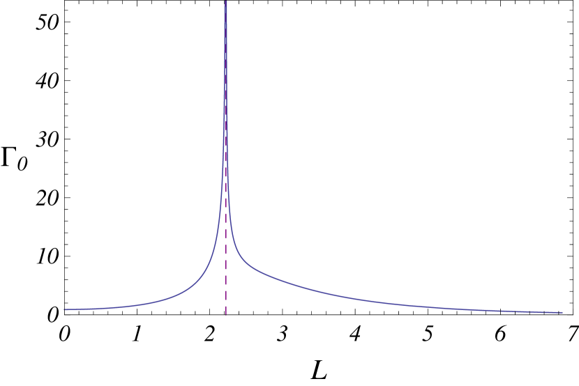
Figure 7: Prefactor $\Gamma_{0}$ vs. $L$ for $\mu_{1}=4$, $\mu_{2}=2$.

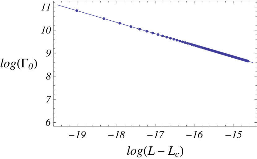
Figure 8: $\log\Gamma_{0}$ vs. $\log(L-L_{c})$ near $L_{c}^{+}$ for $\mu_{1}=4$, $\mu_{2}=2$. The dots indicate numerical data. The line fit gives $\log\Gamma_{0}=-0.5\log(L-L_{c})+1.35$ for $L$ very close to (and above) $L_{c}$.

6 Discussion

We have introduced a stochastic Ginzburg-Landau model with two coupled fields, and have found explicit solutions for the nonuniform saddle states that govern noise-induced transitions from one stable state to another. This model has a phase transition as system size changes, similar to what has been seen in the single-field case [31, 32, 66, 67].

The action functional (4) was designed to model nanowire stability and decay when non-axisymmetric cross sections appear during the time evolution of the wire, either as beginning, ending, or intermediate states. However, the model — or its modifications — has wider applicability, which we briefly discuss below. We note also that the model can be viewed as a generalization of that used by Tarlie et al. [39] to model transitions between different conducting states in superconducting rings.

As noted in Sect. 1, the system analyzed here can serve to model certain transitions among different nanowire states, but not all. Nevertheless, it provides a nice physical interpretation of the escape process in non-axisymmetric nanowires. The escape process occurs, as usual, via nucleation of a “droplet” of one metastable configuration in the background of the other. Fig. 5 indicates that the infinite nanowire begins as a cylindrically symmetric wire at one (uniform) radius and ends as a cylindrically symmetric wire at a different radius, while passing through a sequence of nonaxisymmetric configurations. It is easy to see that if we were to take instead $\mu_{2}>\mu_{1}$, the model would describe a process where the starting and ending states have the same average radius but are non-axisymmetric with different deformation states, while the saddle is cylindrically symmetric. By varying the model parameters, one can interpolate between these two extreme cases. An extensive analysis of such transitions, including applications of the current model, will appear in [48].

The model presented here, or ones close to it, apply also to a variety of other situations. One of these is constrained dynamics of the sort that plays a role in viscous, or glassy, liquids (see, for example, [68, 69]). The simplest situation corresponding to this sort of dynamics is described in Munoz et al. [70]. Fig. 2 of that paper shows a particle attempting to diffuse from one stable position to another; if a second particle is in one of its two stable positions, it blocks the first. Aside from its natural occurrence in glassy liquids, such a situation may also be created and studied using an optical trap with metastable wells, such as that employed by McCann et al. [71] or Seol et al. [72] to test the Kramers transition rate formula under varying conditions.

If one removes the diffusion terms from Eqs. (3), treating $\phi_{1}$ and $\phi_{2}$ simply as spatial coordinates, then one has a model where two degrees of freedom act on each other in a similar manner, although in a mutual fashion (see, for example, [73]). However, inclusion of the diffusion terms describes a more interesting situation. Here one can think of the field $\phi_{1}(z)$ as describing a density of a certain particle species along an interval, and $\phi_{2}(z)$ as representing a second species density. Diffusion of particles into or out of the interval depends on the state of $\phi_{2}(z)$; its vanishing (with the set of parameters used in this paper) “locks” the density of $\phi_{1}(z)$ to one of its stable configurations. In order for any diffusion to take place, $\phi_{2}(z)$ must change also, but its density distribution is coupled to that of $\phi_{1}(z)$. It would be of interest to pursue this further to investigate spatially inhomogeneous models of constrained dynamics.

There are a number of other physical situations that can be stochastically modelled using two coupled classical fields. Examples of such models are the Fitzhugh-Nagumo model [74, 75] describing excitable media in general (and neurons in particular), and the Gray-Scott model [76] of chemical reaction-diffusion systems. These, however, are nonpotential systems, and can exhibit phenomena, such as limit cycles, that potential systems cannot. Nevertheless, if one examines transitions between “fixed points” of such systems, the leading order asymptotics should behave similarly to the model described here. On the other hand, the subdominant asymptotics, for example the prefactor, would require a different approach.

Acknowledgments. The authors are grateful to P. Goldbart and P. Deift for stimulating conversations, and W. Zhang for useful suggestions on programming. This work was supported in part by NSF Grants PHY-0651077 and PHY-0965015.

References

- [1] C. R. Doering, “Modeling complex systems: Stochastic processes, stochastic differential equations, and Fokker–Planck equations,” in 1990 Lectures on Complex Systems (L. Nadel and D. L. Stein, eds.), pp. 3–51, Reading, MA: Addison-Wesley, 1991. Proceedings of the 1990 Complex Systems Summer School (Santa Fe, June 1990).
- [2] C. W. Gardiner, Handbook of Stochastic Methods. New York/Berlin: Springer-Verlag, second ed., 1985.
- [3] W. Horsthemke and R. Lefever, Noise-Induced Transitions: Theory and Applications in Physics, Chemistry, and Biology. New York/Berlin: Springer-Verlag, 1984.
- [4] H. Risken, The Fokker–Planck Equation. Springer-Verlag, second ed., 1989.
- [5] H. R. Brand, C. R. Doering, and R. E. Ecke, “External noise and its interaction with spatial degrees of freedom in nonlinear dissipative systems,” J. Statist. Phys., vol. 54, pp. 1111–1120, 1989.
- [6] Z. Schuss, Theory and Application of Stochastic Differential Equations. New York: Wiley, 1980.
- [7] N. G. van Kampen, Stochastic Processes in Physics and Chemistry. New York/Amsterdam: North-Holland, 1981.
- [8] F. Moss and P. V. E. McClintock, eds., Noise in Nonlinear Dynamical Systems. Cambridge: Cambridge University Press, 1989. Three volumes.
- [9] P. Hänggi, P. Talkner, and M. Borkovec, “Reaction-rate theory: Fifty years after Kramers,” Rev. Mod. Phys., vol. 62, pp. 251–341, 1990.
- [10] P. Talkner and P. Hänggi, eds., New Trends in Kramers’ Reaction Rate Theory. Dordrecht: Kluwer, 1995.
- [11] J. García-Ojalvo and J. M. Sancho, Noise in Spatially Extended Systems. New York/Berlin: Springer, 1999.
- [12] K. Martens, D. L. Stein, and A. D. Kent, “Thermally induced magnetic switching in thin ferromagnetic annuli,” in Noise in Complex Systems and Stochastic Dynamics III (L. B. Kish, K. Lindenberg, and Z. Gingl, eds.), pp. 1–11, SPIE Proceedings Series, 2005.
- [13] K. Martens, D. L. Stein, and A. D. Kent, “Magnetic reversal in nanoscopic ferromagnetic rings,” Phys. Rev. B, vol. 73, p. 054413, 2006.
- [14] M. C. Cross and P. C. Hohenberg, “Pattern formation outside of equilibrium,” Rev. Mod. Phys., vol. 65, pp. 851–1112, 1993.
- [15] Y. Tu, “Worm structure in the modified Swift–Hohenberg equation for electroconvection,” Phys. Rev. E, vol. 56, pp. R3765–R3768, 1997.
- [16] U. Bisang and G. Ahlers, “Thermal fluctuations, subcritical bifurcation, and nucleation of localized states in electroconvection,” Phys. Rev. Lett., vol. 80, pp. 3061–3064, 1998.
- [17] A. M. Dikande, “Microscopic domain walls in quantum ferroelectrics,” Phys. Lett. A, vol. 220, pp. 335–341, 1996.
- [18] D. A. Gorokhov and G. Blatter, “Decay of metastable states: Sharp transition from quantum to classical behavior,” Phys. Rev. B, vol. 56, pp. 3130–3139, 1997.
- [19] J. Bürki, C. A. Stafford, and D. L. Stein, “Theory of metastability in simple metal nanowires,” Phys. Rev. Lett., vol. 95, pp. 090601–1–090601–4, 2005.
- [20] J. Bürki, C. A. Stafford, and D. L. Stein, “Comment on ‘Nonlinear current-voltage curves of gold quantum point contacts’,” Appl. Phys. Lett., vol. 88, p. 166101, 2006.
- [21] J. S. Langer, “Theory of the condensation point,” Ann. Physics, vol. 41, pp. 108–157, 1967.
- [22] J. S. Langer, “Statistical theory of the decay of metastable states,” Ann. Physics, vol. 54, pp. 258–275, 1969.
- [23] S. Coleman, “Fate of the false vacuum: Semiclassical theory,” Phys. Rev. D, vol. 15, pp. 2929–2936, 1977.
- [24] C. G. Callan and S. Coleman, “Fate of the false vacuum, II: First quantum corrections,” Phys. Rev. D, vol. 16, pp. 1762–1768, 1977.
- [25] S. Coleman, “The uses of instantons,” in The Whys of Subnuclear Physics: Proceedings of the 1977 International School (A. Zichichi, ed.), (Erice, Italy), pp. 805–916, Plenum Press, Jul 1977.
- [26] L. S. Schulman, Techniques and Applications of Path Integration. New York: Wiley, 1981.
- [27] W. G. Faris and G. Jona-Lasinio, “Large fluctuations for a nonlinear heat equation with noise,” J. Phys. A, vol. 15, pp. 3025–3055, 1982.
- [28] F. Martinelli, E. Olivieri, and E. Scoppola, “Small random perturbations of finite and infinite dimensional dynamical systems: Unpredictability of exit times,” J. Statist. Phys., vol. 55, pp. 477–504, 1989.
- [29] R. Forman, “Functional determinants and geometry,” Invent. Math., vol. 88, pp. 447–493, 1987.
- [30] A. J. McKane and M. B. Tarlie, “Regularization of functional determinants using boundary perturbations,” J. Phys. A, vol. 28, pp. 6931–6942, 1995.
- [31] R. S. Maier and D. L. Stein, “Droplet nucleation and domain wall motion in a bounded interval,” Phys. Rev. Lett., vol. 87, pp. 270601–1–270601–4, 2001.
- [32] D. L. Stein, “Critical behavior of the Kramers escape rate in asymmetric classical field theories,” J. Statist. Physics, vol. 114, pp. 1537–1556, 2004.
- [33] I. Affleck, “Quantum-statistical metastability,” Phys. Rev. Lett., vol. 46, pp. 388–391, 1981.
- [34] P. G. Wolynes, “Quantum theory of activated events in condensed phases,” Phys. Rev. Lett., vol. 47, pp. 968–971, 1981.
- [35] H. Grabert and U. Weiss, “Crossover from thermal hopping to quantum tunneling,” Phys. Rev. Lett., vol. 53, pp. 1787–1790, 1984.
- [36] E. M. Chudnovsky, “Phase transitions in the problem of decay of a metastable state,” Phys. Rev. A, vol. 46, pp. 8011–8014, 1992.
- [37] A. N. Kuznetsov and P. G. Tinyakov, “Periodic instanton bifurcations and thermal transition rate,” Phys. Lett. B, vol. 406, pp. 76–82, 1997.
- [38] J. Bürki, C. A. Stafford, and D. L. Stein, “The order of phase transitions in barrier crossing,” Phys. Rev. E, vol. 77, p. 061115, 2008.
- [39] M. Tarlie, E. Shimshoni, and P. Goldbart, “Intrinsic dissipative fluctuation rate in mesoscopic superconducting rings,” Phys. Rev. B, vol. 49, pp. 494–497, 1994.
- [40] G. Rubio, N. Agraït, and S. Vieira, “Atomic-sized metallic contacts: Mechanical properties and electronic transport,” Phys. Rev. Lett., vol. 76, pp. 2302–2305, 1996.
- [41] A. Stalder and U. Dürig, “Study of yielding mechanics in nanometer-sized Au contacts,” Appl. Phys. Lett., vol. 68, pp. 637–639, 1996.
- [42] J. M. Krans, J. M. van Ruitenbeek, and L. J. de Jongh, “Atomic structure and quantized conductance in metal point contacts,” Physica B, vol. 218, pp. 228–233, 1996.
- [43] Y. Kondo and K. Takayanagi, “Gold nanobridge stabilized by surface structure,” Phys. Rev. Lett., vol. 79, pp. 3455–3458, 1997.
- [44] H. Ohnishi, Y. Kondo, and K. Takayanagi, “Quantized conductance through individual rows of suspended gold atoms,” Nature, vol. 395, pp. 780–782, 1998.
- [45] H. E. van den Brom, A. I. Yanson, and J. M. van Ruitenbeek, “Characterization of individual conductance steps in metallic quantum point contacts,” Physica B, vol. 252, pp. 69–75, 1998.
- [46] A. I. Yanson, I. K. Yanson, and J. M. van Ruitenbeek, “Observation of shell structure in sodium nanowires,” Nature, vol. 400, pp. 144–146, 1999.
- [47] Y. Kondo and K. Takayanagi, “Synthesis and characterization of helical multi-shell gold nanowires,” Science, vol. 289, pp. 606–608, 2000.
- [48] J. Bürki, L. Gong, C. A. Stafford, and D. L. Stein in preparation.
- [49] F. Kassubek, C. A. Stafford, J. Bürki, and H. Grabert, “Universality in metallic nanocohesion: A quantum chaos approach,” Phys. Rev. Lett., vol. 83, pp. 4836–4839, 1999.
- [50] M. E. T. Molares, A. G. Balogh, T. W. Cornelius, R. Neumann, and C. Trautmann, “Fragmentation of nanowires driven by Rayleigh instability,” Appl. Phys. Lett., vol. 85, pp. 5337–5339, 2004.
- [51] F. Kassubek, Electrical and Mechanical Properties of Metallic Nanowires. Inaugural dissertation zur erlangung der doktorwürde, Albert-Ludwigs-Universität, Freiburg, Germany, Dept. of Physics, October 2000.
- [52] F. Kassubek, C. A. Stafford, H. Grabert, and R. E. Goldstein, “Quantum suppression of the Rayleigh instability in nanowires,” Nonlinearity, vol. 14, pp. 167–177, 2001.
- [53] C. A. Stafford, F. Kassubek, and H. Grabert, “Cohesion and stability of metal nanowires: A quantum chaos approach,” in Advances in Solid State Physics, Vol. 41 (B. Kramer, ed.), pp. 497–511, Berlin: Springer-Verlag, 2001.
- [54] A. I. Yanson, I. K. Yanson, and J. M. van Ruitenbeek, “Supershell structure in alkali metal nanowires,” Phys. Rev. Lett., vol. 84, pp. 5832–5835, 2000.
- [55] A. I. Yanson, J. M. van Ruitenbeek, and I. K. Yanson, “Shell effects in alkali metal nanowires,” Low Temp. Phys., vol. 27, pp. 807–820, 2001.
- [56] J. Bürki, C. A. Stafford, and D. L. Stein, “Fluctuational instabilities of alkali and noble metal nanowires,” in Noise in Complex Systems and Stochastic Dynamics II (Z. Gingl, J. M. Sancho, L. Schimansky-Geier, and J. Kertesz, eds.), pp. 367–379, SPIE Proceedings Series, 2004.
- [57] D. F. Urban, J. Bürki, C.-H. Zhang, C. A. Stafford, and H. Grabert, “Jahn-Teller distortions and the supershell effect in metal nanowires,” Phys. Rev. Lett., vol. 93, pp. 186403–1–186403–4, 2004.
- [58] D. F. Urban, J. Bürki, C. A. Stafford, and H. Grabert, “Stability and symmetry breaking in metal nanowires: The nanoscale free-electron model,” 2006.
- [59] C. A. Stafford, D. Baeriswyl, and J. Bürki, “Jellium model of metallic nanocohesion,” Phys. Rev. Lett., vol. 79, pp. 2863–2866, 1997.
- [60] J. Bürki, R. E. Goldstein, and C. A. Stafford, “Quantum necking in stressed metallic nanowires,” Phys. Rev. Lett., vol. 91, pp. 254501–1–254501–4, 2003.
- [61] R. S. Maier and D. L. Stein, “Effects of weak spatiotemporal noise on a bistable one-dimensional system,” in Noise in Complex Systems and Stochastic Dynamics (L. Schimansky-Geier, D. Abbott, A. Neiman, and C. V. den Broeck, eds.), pp. 67–78, Singapore: SPIE, 2003.
- [62] M. Abramowitz and I. A. Stegun, eds., Handbook of Mathematical Functions. New York: Dover, 1965.
- [63] I. M. Gelfand and A. M. Yaglom, “Integration in functional spaces and its applications in quantum physics,” J. Math. Phys, vol. 1, pp. 48–69, 1960.
- [64] K. Kirsten and A. J. McKane, “Functional determinants by contour integration methods,” Ann. Phys., vol. 308, p. 520, 2003.
- [65] P. Hartman, Ordinary Differential Equations. Birkhäuser, Second ed., 1982.
- [66] R. S. Maier and D. L. Stein, “Effects of weak spatiotemporal noise on a bistable one-dimensional system,” in Noise in Complex Systems and Stochastic Dynamics (L. Schimansky-Geier, D. Abbott, A. Neiman, and C. V. den Broeck, eds.), vol. 5114, pp. 67–78, SPIE Proceedings Series, 2003.
- [67] D. L. Stein, “Large fluctuations, classical activation, quantum tunneling, and phase transitions,” Braz. J. Phys., vol. 35, pp. 242–252, 2005.
- [68] R. G. Palmer, D. L. Stein, E. Abrahams, and P. Anderson, “Models of hierarchically constrained dynamics for glassy relaxation,” Phys. Rev. Lett., vol. 53, pp. 958–961, 1984.
- [69] G. H. Fredrickson and H. C. Andersen, “Kinetic Ising model of the glass-transition,” Phys. Rev. Lett., vol. 53, pp. 1244–1247, 1984.
- [70] M. A. Munoz, A. Gabrielli, H. Inaoka1, and L. Pietronero, “Hierarchical model of slow constrained dynamics,” Phys. Rev. E, vol. 57, pp. 4354–4360, 1998.
- [71] L. I. McCann, M. I. Dykman, and B. Golding, “Thermally activated transitions in a bistable three-dimensional optical trap,” Nature, vol. 402, pp. 785–787, 1999.
- [72] Y. Seol, D. L. Stein, and K. Visscher, “Phase measurements of barrier crossings in a periodically modulated double-well potential,” Phys. Rev. Lett., vol. 103, p. 050601, 2009.
- [73] R. S. Maier and D. L. Stein, “Transition-rate theory for nongradient drift fields,” Phys. Rev. Lett., vol. 69, pp. 3691–3695, 1992. In this paper an asymmetric, quasi- version of a blocking model was discussed.
- [74] R. FitzHugh, “Mathematical models of threshold phenomena in the nerve membrane,” Bull. Math. Biophysics, vol. 17, pp. 257–278, 1955.
- [75] J. Nagumo, S. Arimoto, and S. Yoshizawa, “An active pulse transmission line simulating nerve axon,” Proc. IRE, vol. 50, pp. 2061–2070, 1962.
- [76] J. Pearson, “Complex patterns in a simple system,” Science, vol. 261, pp. 189–192, 1993.