Employer Expectations, Peer Effects and Productivity:
Evidence from a Series of Field Experiments

Abstract

This paper reports the results of a series of field experiments designed to investigate how peer effects operate in a real work setting. Workers were hired from an online labor market to perform an image-labeling task and, in some cases, to evaluate the work product of other workers. These evaluations had financial consequences for both the evaluating worker and the evaluated worker. The experiments showed that on average, evaluating high-output work raised an evaluator’s subsequent productivity, with larger effects for evaluators that are themselves highly productive. The content of the subject evaluations themselves suggest one mechanism for peer effects: workers readily punished other workers whose work product exhibited low output/effort. However, non-compliance with employer expectations did not, by itself, trigger punishment: workers would not punish non-complying workers so long as the evaluated worker still exhibited high effort. A worker’s willingness to punish was strongly correlated with their own productivity, yet this relationship was not the result of innate differences—productivity-reducing manipulations also resulted in reduced punishment. Peer effects proved hard to stamp out: although most workers complied with clearly communicated maximum expectations for output, some workers still raised their production beyond the output ceiling after evaluating highly productive yet non-complying work products.

JEL J01, J24, J3

1 Introduction

A perennial question of interest to both economists and firm managers alike is why employees work hard despite facing weak incentives and light monitoring. Many theories have been proposed: firms might obtain high effort via explicit contracts (Holmstrom, 1982), relational contracts (Levin, 2003) or efficiency wages (Katz, 1986). In each of these theories, the explanation hinges upon the relationship between the firm and the individual worker—a worker’s co-workers or “peers,” if they matter at all, are relevant only to the extent that they influence the incentives offered by the firm (e.g., by influencing payoffs in a relative performance scheme). However, recent empirical research has highlighted the direct effects that co-workers can have on each others productivity without intermediation by the firm. There are several potential channels through which these workplace peer effects could flow: peers could offer instruction about how to be more productive, threaten punishment, promise rewards, offer examples of relevant norms or spur competition. The purpose of this paper is to help clarify these potential mechanisms through experimentation in a real work setting.

1.1 Overview of experiments and findings

This paper reports the results of five closely related field experiments designed to explore the relationships among a worker’s peers, the policies and statements of the firm and a worker’s productivity. Table 1 provides an overview of each experimental design and the results. In each experiment, workers from an online labor market were hired to produce descriptive labels for photographic images. In each experiment, all subjects labeled the exact same image which makes output comparisons across experimental groups meaningful. Before joining the experiment, would-be workers read a description of the task, learned the payment and viewed a work sample (i.e., a screen shot of the image-labeling interface with some number of labels completed). If they chose to participate, they labeled one or more images, depending on the details of the experiment. A worker’s output was simply the number of labels they produced. Because subjects were not informed they were participating in experiments, the experiments were “natural” field experiments in the Harrison and List (2004) taxonomy.

In Experiment A, subjects were randomly assigned to view either a high-output work sample (with many labels for an image) or a low-output work sample (with only a few labels for that same image). All subjects then performed an image-labeling task. All subjects labeled the same image, making cross-group output comparisons meaningful. Exposure to the high-output work sample lowered labor supply on the extensive margin but raised it on the intensive margin. These two results are important for follow-on experiments, because they imply that (1) subjects regarded effort as costly and (2) subjects held the work sample as informative about employer expectations.

In Experiment B, all subjects viewed the same low-output work sample from Experiment A and then completed an image-labeling task. After completing this task, subjects evaluated the work of another worker. The evaluated work displayed either high- or low-output, and subjects were randomly assigned to the work they evaluated. Evaluation had two parts: each subject was asked to recommend whether or not the firm should “approve” the evaluated work as well as how to split a bonus with the evaluated worker. The bonus split question created a contextualized dictator game. The “approve” question has a technical and consequential meaning in the market—when work is not approved, the worker submitting that work does not get paid and their reputation suffers. Evaluating low-output work led to greater punishment: subjects viewing low-output work were far more likely to recommend rejection and granted smaller bonuses. Regardless of group assignment, highly productive subjects (as measured by their output on the initial task) were harsher judges; compared to their low-productivity peers, they were more likely to recommend rejection and they granted smaller bonuses.

All subjects in Experiment C were first shown a low productivity work sample. Subjects then performed an image-labeling task. After completing the task, subjects next evaluated the work product of another worker. Unlike in Experiment B, all subjects in C evaluated the same work. The only experimental manipulation in Experiment C occurred during the image-labeling phase: subjects were randomly assigned to either a normal image-labeling interface or to a special image-labeling interface that generated a pop-up notice after subjects added their second label. This pop-up notice was designed to modify subjects’ beliefs about employer expectations. The purpose of the notice was to reduce output without inducing a change in extensive labor supply. By changing output without changing the composition of subjects (i.e., no supply effects on the extensive margin), it was possible to test the “innate types” explanation for the strong relationship between productivity and punishment found in Experiment B. In this experiment, I found no evidence that highly productive workers are simply more punishment prone: workers receiving the pop-up notice reduced their output, decreased their rejection recommendations and increased their bonuses.

In Experiment D, all subjects were first shown a low productivity work sample. Next, they performed an initial image labeling task and then were randomly assigned to evaluate either high- or low-output work. After this evaluating, subjects performed an additional image-labeling task. On average, workers that evaluated highly productive work produced more labels in the follow-on image-labeling task than workers that evaluated less productive work. These effects on productivity were strong and easily detectable, but they were not homogeneous: less productive workers were far less susceptible to the effects, contra to some findings that peer effects raise the output of low productivity workers (Falk and Ichino, 2006; Mas and Moretti, 2009).

In Experiment E all subjects were shown a work sample with exactly $2$ labels and were told that they should produce only $2$ labels. After performing an initial image-labeling task, subjects evaluated work that contained either $2$ or $11$ labels. Workers did not treat the high-effort but non-complying work as worthy of punishment: subjects were just as likely to recommend approval of the $11$ label work and granted slightly larger bonus payments. Despite the explicit statements of employer expectations, exposure to the high-output/non-complying work had the same effect as exposure to high-output work in Experiment D: exposed workers raised output, in many cases beyond the clearly communicated ceiling. However, most workers complied with the standard initially, and exposure to complying work seemed to further increase compliance.

1.2 Implications

One explanation for the results across the five experiments is that workers were uncertain about what constituted an appropriate amount of output and they use observations from employer-provided work samples and the output of peers to determine that amount. Because workers find labeling costly, these beliefs about employer expectations serve as a constraint in the implicit optimization problem faced by workers.

Learning about employer expectations results in changes not only in a worker’s labor supply, but also in their willingness to punish or reward their peers. As this learning can come from multiple sources, perceived employer expectations do not fall wholly under any single entity’s control and can evolve as workers work, observe, and are observed.

Punishment seems to come easily to many workers. The reasons why workers punish is unclear, but there are several possible theoretical explanations. Perhaps the simplest is that workers view themselves as a monitored agent of the employer, and they make decisions about acceptance and bonuses according to what they believe will satisfy the principal. However, workers do not appear to be general-purpose enforcers of employers’ requests—workers punish low effort. Non-complying but high effort work is treated no differently vis-à-vis punishment than complying work. The fact that workers only appear willing to punish low effort places a constraint on how firms can make use of worker-driven norm enforcement. For example, it may be difficult to get workers to substitute easy, correct procedures for difficult, inefficient procedures. Ironically, the difficulty itself might make an outdated procedure harder to replace, as workers who adopt the easier method might be perceived to be shirking.

The finding that exposure to low-output work lowers output, combined with the finding that low-productivity reduces willingness to punish, suggests the possibility of an organizational vicious cycle: after observing idiosyncratically bad work, workers may lower their own output and punish less in response, in turn reducing other workers’ incentives to be highly productive. This may explain why organizational leaders often use the language of contagion to describe morale and so much of management theory focuses on understanding and influencing organizational culture (Schein, 2004), rather than, for example, trying to write perfectly complete employment contracts.

1.3 Related work

Several recent papers examine the effects of peers on workplace productivity. Perhaps the most illuminating observational evidence comes from Mas and Moretti (2009), who showed that less productive grocery clerks exhibited greater productivity when working near highly productive clerks, but only when they were in the direct view of the highly productive clerks. This finding suggests that the threat of punishment might partially explain workplace peer effects. There is much laboratory literature supporting this punishment-as-peer-effect view, with several studies showing that workers will readily bear costs and altruistically punish peers that free-ride in public goods games (Fehr and Gachter, 2002, 2000). This “strong reciprocity” (Carpenter et al., 2009) is a powerful peer effect, and although firms are not perfectly analogous to public goods games, the notion of worker-enforced productivity norms offers a very general potential solution to the incentive problem of team production.

Guryan, et al. (2009) also use evidence from a real workplace, albeit an unusual one: they exploited the random assignment of professional golfers to tournament foursomes to estimate the effects of each player’s peers on the player’s own performance. In contrast to Mas and Moretti, Guryan, et al. found no evidence of peer effects, providing a useful corrective to hasty or overly broad generalizations. However, professional golf tournaments are unusual work environments, in that two common channels for peer effects are foreclosed: professional golfers know what constitutes good performance and are unlikely to raise their quality of play in the “shadow” of punishment that might be meted out for non-compliance with productivity norms. In marked contrast with the Mas and Moretti setting, shirking by a professional golfer imposes a positive externality on “co-workers.”

Using a field experiment, Falk and Ichino (2006) showed that workers stuffing envelopes in pairs had less variation in their output levels than synthetically “paired” workers constructed from an experimental group whose members worked alone. While they cannot estimate the direction of peer effects (i.e., low productivity affects or is affected by high productivity, or some amalgamation of effects), their analysis of the output distribution led them to conclude that it was more likely that less productive workers were made more productive by working in pairs.

The difference between the Guryan, et al. setting, the Falk and Ichino setting and that of Mas and Moretti—and the resultant difference in findings—serves as a justification for the present study, which has an unusual but highly controllable work context that preserves some of the common features of work environments, including uncertainty about norms, costly effort and a task unlikely to inspire much intrinsic motivation. Unlike the Mas and Moretti setting, however, there are no overt free-riding externalities (in the check-out line, slacking by one clerk increases the work load of other clerks). The absence of direct negative externalities is important, as evidence from such a setting can provide some sense of how general punishment might operate in the workplace.

1.4 Contribution

This paper contributes to the emerging literature on workplace peer effects. It provides credible evidence of the existence and operation of peer effects on productivity, which is especially useful given the lack of concordance between some of the major results in the field and the inherent difficulty of estimating these kinds of effects (Manski, 1993). This evidence is particularly useful because the scope of possible interpretations is limited, due to the narrow channel through which peer effects could operate. Observation of work output was the only “interaction” and the payment scheme was not relative. The punishment component provides additional insight into the shadow cast by peer-based norm enforcement.

One methodological advance of this paper is that productivity is measured both before and after exposure to peers. By base-lining prior output, the conditional nature of peer effects becomes apparent. For example, I find that the conditional treatment effects of exposure to low quality peers differ from the effects found by Falk and Ichino. They found that “bad apples far from damaging good apples seem instead to gain in quality when paired with the latter.” Mas and Moretti find a similar result. In the setting examined here, the traditional bad apples metaphor applied—the bad apples ruined the good apples, and the good apples did nothing for the bad.

2 Methods and Materials

Before describing the experiment results, I first describe the marketplace where the experiments were conducted, the methodological issues involved in online experimentation and the actual task completed by workers and interface used. The experiments were conducted on Amazon’s Mechanical Turk (MTurk), an online labor market where workers are available to complete small tasks for payment. Background information on MTurk closely follows Horton and Chilton (2010). MTurk is one of several online labor markets that have emerged in recent years (Frei, 2009). At present, it is the most amenable to online experimentation.

Table 1: Details of the Experiments

Exp.	Question	Set-up	Treatment	Control	Result
A	Can employers convey productivity expectations?	Subjects viewed an employer-provided work sample, then chose how many labels to produce (if any). Work samples differed by experimental group.	HIGH:Subjects viewed high-output work sample (many labels)	LOW: Subjects viewed low-output work sample (few labels)	HIGH increased labor supply on intensive margin, but decreased it on extensive margin
B	Do workers punish workers that exhibit low productivity?	Subjects viewed an employer-provided work sample, then chose how many labels to produce. Subjects then evaluated another worker’s work product.	GOOD: Subjects evaluated a high-output work sample	BAD: Subjects evaluated a low-output work sample	GOOD increased approval recommendations and bonus amounts. Highly productive workers punished more with their evaluations.
C	Is the relationship between own-productivity and punishment causal?	Subjects viewed an employer-provided work sample, then chose how many labels to produce. Subjects then evaluated another worker’s work product.	CURB: Subjects received a notice after two labels saying that 3 labels was probably enough output	NONE: Subjects received no notice.	Greatly reduced output in CURB; those in CURB more likely to recommend approval and grant larger bonuses
D	Does exposure to low-output work affect a worker’s productivity?	Subjects viewed an employer-provided work sample, then chose how many labels to produce. Subjects then evaluated another worker’s work product. Then they labeled a second image.	GOOD: Subjects evaluated a high-output work sample	BAD: Subjects evaluated a low-output work sample	GOOD raised output on second task; effects were stronger for more productive subjects (measured by first task output).
E	Are workers susceptible to peer effects in presence of strongly-stated employer expectations? Do they punish high-effort but non-complying work?	Subjects viewed an employer-provided work sample with 2 labels, then chose how many labels to produce. Subjects were told that 2 and only 2 labels should be produced. Subjects then evaluated another worker’s work product, then labeled a second image.	OVER: Subjects evaluated a worker producing too many labels	OK: Subjects evaluated a worker producing the required number of labels	OVER increased subsequent output beyond ceiling, but did not cause more punishment.

2.1 Online experimentation

In the past few years, researchers in a number of disciplines—with computer science leading the way—have begun running experiments online using online labor markets. Some examples in economics include Mason and Watts (2009), Chandler and Kapelner (2010) and Horton and Chilton (2010). Horton, Rand and Zeckhauser (2010) argue that online experiments can offer a high degree of both internal and external validity. Despite their advantages online experiments can also be harder to control compared to conventional laboratory experiments. However, they are generally easier to control than conventional field experiments. Because subjects may quit at any time, the biggest threat to valid inference is non-random attrition. In Experiment A, quitting was actually a useful outcome to observe, as the experiment focused on labor supply on both the intensive and extensive margins. In the other four experiments, by design, essentially all attrition occurred before subjects experienced any treatment-specific differences. For Experiments B-E, only subjects that completed the initial image-labeling task were included in the sample (with others dropped), but this creates no sampling bias, since all subjects made their initial output decisions before being exposed to any experimental group-specific treatments.

2.2 Amazon’s Mechanical Turk

Amazon’s Mechanical Turk is an online labor market where workers are available to perform small jobs called “Human Intelligence Tasks” (HITs) for buyers, who, in the parlance of MTurk, are called “requesters.” HITs vary, but most are small, simple tasks that are difficult for computers but relatively easy for humans to perform. Common tasks include transcribing audio clips, classifying and tagging images, reviewing documents and checking websites for pornographic content. When posting a HIT, a requester describes the task, creates a user interface, establishes a piece-rate payment, specifies worker qualifications, and sets the number of times each HIT may be performed.

In order to become an MTurk worker, a person must create an MTurk account and provide a bank account number to Amazon. Workers are only allowed to have one account, and Amazon uses several technical and legal means to enforce this restriction. Once they are members, workers are able to observe the collection of HITs available to them and, in most cases, view a sample of the required work. They can work on any task for which they are qualified and can begin work immediately after accepting a HIT.

Once a worker completes a HIT, the work product is submitted to the requester for review. The requester decides whether or not to “approve” it. If approved, the worker is paid the piece rate. The worker is also paid if the requester does not review and approve the work within a specified amount of time. Solely at their discretion, requesters may “reject” work, in which case the worker is not paid. The ability of requesters to reject work creates consequences for providing work that does not meet employer expectations—a feature critical to the experiments conducted. Requesters may also elect to pay bonuses, which makes it easy to tailor payments to individual workers based on their performance within a nominally piece-rate HIT.

MTurk workers appear to be split approximately evenly between the US and India. Most report that they participate to earn money and generally view employers online as having the same level of trustworthiness as offline, traditional employers (Horton, 2010b). For the demographics of the MTurk population, see Ipeirotis (2010).

2.3 Task and interface

In each of the experiments, subjects were asked to label images. The images themselves were selected from the photo sharing website Flickr. Image-labeling is a very common “human computation” task because labels are needed to make images searchable, but computers do a poor job of identifying objects in images (von Ahn and Dabbish, 2004; Huang et al., 2010). The interface itself was created in Limesurvey, an open-source survey platform. In order to add labels, subjects had to click a button labeled “Add a label.” A screen shot of the interface can be seen in Figure 1. Clicking the button caused a new blank text field to be added to the survey. When they finished adding labels subjects clicked a button labeled “Submit labels,” which saved within the survey all of the labels generated and the time spent adding labels. No attempt was made to adjudicate the quality of the labels—if the subject started to add another label, this was recorded as an additional unit of output.

For the evaluation task, each subject viewed a screen shot of another worker’s work product. As with the initial image-labeling task, the evaluation task (and the potential bonus) was likely perceived as unextraordinary. On MTurk, it is very common to have workers evaluate the work of other MTurk workers. A frequently used solution to the problem of spam submissions (which occur often when buyers post many tasks—see Ipeirotis et al. (2010)) is to have workers vote on the work product of other workers. It is also very common to use bonuses to motivate performance.

It is important to note that all the subjects in an experiment labeled the same image, regardless of their group assignment. For example, in Experiment A, all subjects labeled an image showing a collection of mechanics tools. What varied across experimental groups were factors like the provided work sample, work instructions or the demonstrated productivity of the worker they were asked to evaluate. Because the images were the same across groups, output levels are comparable, and differences in output can be attributed causally to whatever factor was manipulated in that experiment.

2.4 Demographic survey

In each of the five experiments, subjects answered a short demographic survey before beginning work. The survey was identical in each experiment. Subjects were asked to report their gender, country (choices were US, India or some other country) and whether they use MTurk primarily in order to make money, learn new skills or have fun. There were small differences in the reported covariates across experiments, with most of the difference probably driven by differences in when experiments were launched.

Although one might think the survey would rise suspicions that the task was an experiment, I view this as unlikely. Asking workers for basic demographic information is fairly common in the market, as requesters frequently use location and formal qualifications to screen workers. In fact, place- and reputation-based screening is built into the system, making it even more likely that workers view the demographic questions as an employer work-around to further expand the ability to screen or algorithmically adjudicate response quality. With some noted exceptions, the demographic information had little predictive power and only marginally improved the precision in the regressions, so they were not included.

3 Experiment A: Perceived employer expectations

Experiment A investigates whether a “firm” in this market can influence employee expectations about productivity. For the image labeling task, a simple way to convey expectations is to show a work sample. In this experiment, workers were assigned to one of two experimental groups: $HIGH$, in which the work sample showed $9$ labels, and $LOW$, in which the work sample showed $2$ labels. The work samples are shown in Figure 1. After subjects viewed their assigned work sample, they chose to either label an image or exit the experiment, forfeiting payment.

Table 2 shows the summary statistics for the experiment. The job posting explained that workers would be asked to do a simple image-labeling task and would be paid 30 cents. The planned sample size was 100. Subjects not completing the demographic survey (which occurred prior to group assignment) were dropped from the sample. In this experiment and all subsequent experiments, subjects were assigned to groups by stratifying on arrival time (e.g., subject 1 was assigned to $HIGH$, subject 2 to $LOW$, subject 3 to $HIGH$ and so on).

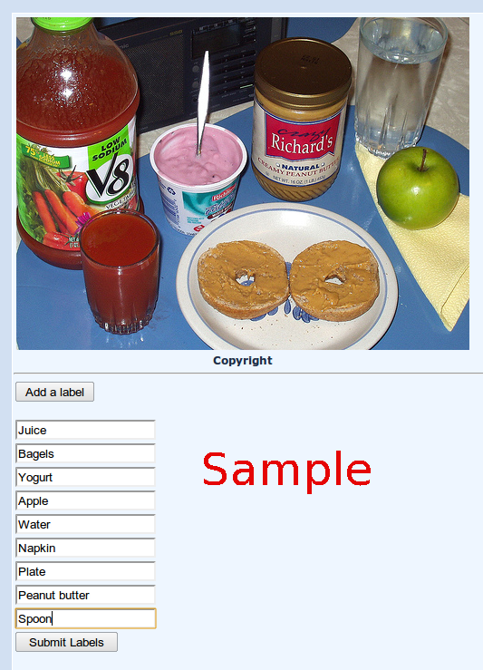
(a)

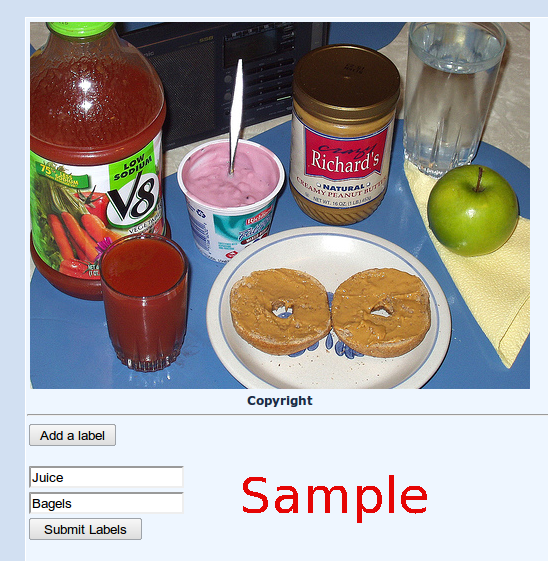
(b)

Figure 1: Work samples shown to workers prior to task acceptance in Experiment A.

Table 2: Experiment A summary statistics ($n=93$)

Administrative
Launch: Fri Apr 09 21:10:31 GMT 2010
Finish: Sun Apr 11 10:04:40 GMT 2010
Survey	FALSE	TRUE	% TRUE
male	39	54	58.1
from India	48	45	48.4
from US	58	35	37.6
motivated by money	22	71	76.3
Treatment Assignment
$HIGH=1$	47	46	49.5
Output	Min	.25	Med.	Mean	.75	Max
Labels produced ($y$)
in HIGH	0	0	1	4.609	8.5	20
in LOW	0	1	2	2.638	3	13
Entry ($y>0$)
in HIGH	0	0	1	0.6957	1	1
in LOW	0	1	1	0.8723	1	1
Time spent on task (seconds)
in HIGH	9.157	53.27	98.13	172.9	225.4	715.5
in LOW	9.563	28.61	54.9	94.85	110.4	904.3

The key result from Experiment A can be seen in the differences in group means in the “Labels produced” and the “Entry” rows.

3.1 Results

The main results from the experiment are displayed in Figure 2, which shows histograms of output for each experimental group. Mean output is indicated via a vertical line in each panel. Subjects in $HIGH$ produced absolutely more output. A sizable number of subjects in $HIGH$ produced more than $12$ labels, but only 1 subject in $LOW$ produced more than $12$ labels. However, the greater productivity in $HIGH$ came at a cost: a larger fraction of subjects in $HIGH$ elected not to produce any output and quit.

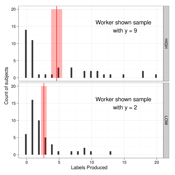
Figure 2: Histogram of labels produced by experimental group in Experiment A. The solid vertical line indicates the mean, while the shaded band around that line is $2$ standard errors wide. Subjects in the $HIGH$ group were shown a work sample consisting of $9$ labels prior to performing, while subjects in $LOW$ were shown a work sample with only $2$ labels. The right edge of each bar intersects the x-axis at the corresponding member of the support, i.e., the largest output choice in the $HIGH$ panel is $y=20$. This plot and all plots in the document were made using the open source R package ggplot2 (Wickham, 2008).

3.1.1 High employer expectations reduced labor supply on the extensive margin

When we regress an indicator for any output at all on the treatment indicator, we have:

$$1\{y>0\}=\underbrace{-0.177}_{[0.085]}\cdot HIGH+\underbrace{0.872}_{[0.050]}$$ (1)

with $n=93$ and $R^{2}=0.05$. Subjects assigned to $HIGH$ were significantly less likely to accept the task compared to subjects in $LOW$.

3.1.2 High employer expectations increased labor supply on the intensive margin

Despite the much greater number of subjects in $HIGH$ who chose not to participate (and thus provided $0$ labels), output was unconditionally higher in $HIGH$ than in $LOW$. Even with the non-participants included as $y=0$ observations, subjects in $HIGH$ produced, on average, roughly $2$ more labels per person:

$$y=\underbrace{1.970}_{[0.956]}\cdot HIGH+\underbrace{2.638}_{[0.430]}$$ (2)

with $n=93$ and $R^{2}=0.05$.

3.2 Discussion

Experiment A suggests that workers use the work sample to infer how much work will be required to meet the employer’s expectations and thus obtain payment. Given that buyers can reject submitted work, the labor supply results are consistent with workers viewing label creation as costly. Some of the subjects decided that the costs of meeting the perceived requirements for the $HIGH$ group were too high and chose to exit. Those subjects that stayed worked to the higher perceived standard and completed the task. The increase in output in $HIGH$ was the result of some combination of selection and greater effort. Because unconditional output rose significantly in $HIGH$, we know that selection alone cannot explain the increase in output.

The results highlight the trade-off firms might face when communicating standards to employees. Claiming to have high standards may be counterproductive, depending on the nature of the firm’s demand for labor. In our particular image-labeling application, conveying high standards via the highly productive work sample was efficient only if the goal was to minimize the per-label price, but it is easy to imagine scenarios where this is not the objective. For tasks like image-labeling, obtaining a large and diverse pool of workers—each contributing a relatively small amount of outut—may be more useful than obtaining lots of output from small number of workers , in which case the high standards conveyed to $HIGH$ would have been undesirable.

4 Experiment B: Punishment and peer output

Experiment B investigated the conditions under which workers reward or punish their fellow workers on the basis of their co-workers output. Subjects in the Experiment first completed an image-labeling task and then were randomly assigned to either the $GOOD$ or the $BAD$ experimental group. The $GOOD$ subjects inspected the output of a worker from Experiment A that produced 12 unique labels while $BAD$ subjects inspected the output of a worker that produced only $1$ unique label. The output samples of the evaluated workers are shown in Figure 3. Subjects were then asked to (1) give a recommendation as to whether or not the work inspected should be approved and (2) decide how to split a $9$ cent bonus with the evaluated worker. Specifically, subjects were asked, “Should we approve this work?” and had to answer “yes” or “no.” Both questions were asked on the same survey page, and subjects could answer them in either order, though the approval question was first on the page. In the regressions that follow, $approve=1$ indicates that a subject recommended approval. For the contextualized dictator game, subjects were told:

“We want to determine how good this work is. We would like you to decide, based on your work and the quality of the other work, how to split a 9 cent bonus.”

Subjects selected an answer from a list of $9$ options of the form “X cents for them, $9-X$ cents for me,” with X ranging from $0$ to $9$ ($9$ cents was chosen as the endowment to reduce the salience of the focal point 50-50 split). At the end of the experiment, we implemented all choices, with bonuses paid to the evaluating subjects and to the two lucky subjects responsible for the $GOOD$ and $BAD$ evaluated work samples. In the regressions that follow, the amount transferred to the evaluated subject is represented by $bonus$, with $bonus\in[0,9]$.

The MTurk job posting for Experiment B was nearly identical to the posting for Experiment A, except that potential subjects were told that they would be evaluating the work of another worker. Before accepting the task, all subjects were shown the $HIGH$ work sample used in Experiment A. Because of the additional evaluation work, the participation payment was raised from 30 cents to 40 cents. The requested sample size was also increased to 200. Table 3 reports the summary statistics for Experiment B.

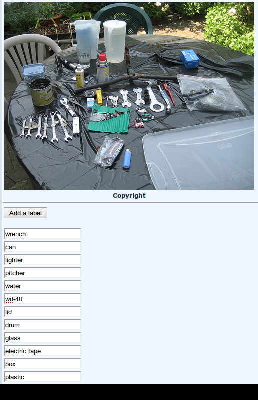
(a)

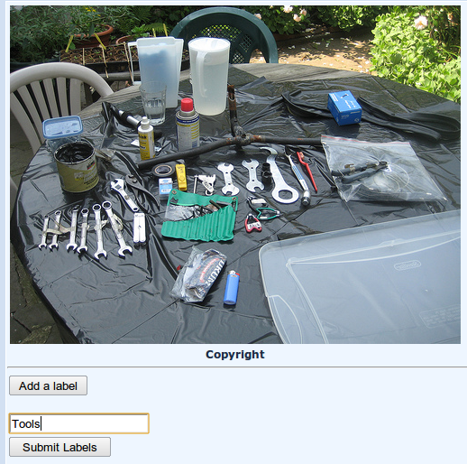
(b)

Figure 3: Work evaluated by subjects in Experiment B

Table 3: Experiment B summary statistics ($n=167$)

Administrative
Launch: Sun Apr 11 04:36:25 GMT 2010
Finish: Mon Apr 12 12:39:20 GMT 2010
Survey	FALSE	TRUE	% TRUE
male	70	97	58.1
from India	92	75	44.9
from US	118	49	29.3
motivated by money	41	126	75.4
Treatment Assignment
$GOOD=1$	82	85	50.9
Recommended firm approve work
in GOOD	7	78	91.8
in BAD	41	41	50
Bonus to evaluated worker	Min	.25	Med.	Mean	.75	Max
in GOOD	0	4	5	4.929	6	9
in BAD	0	1	3	3.488	5	9

Notes: Overlap in subjects across experiments was $|A\cap B|=15$. Subjects in $GOOD$ evaluated work displaying 12 labels, while subjects in $BAD$ evaluated work displaying only $1$ label. The key results from the experiments can be seen in the group proportion differences in the “Recommended firm approve work” rows (in the %TRUE column) and the group mean differences in the “Bonus to evaluated worker” rows.

4.1 Results

The results from Experiment B can be seen in Figure 4, which contains 4 histograms, each showing the allocation of the $9$-cent bonus. The plots are faceted by experimental group (row) and subject recommendation regarding approval (column). We can see that subjects in $GOOD$ were very unlikely to recommend rejection, whereas recommendations for rejection were fairly common among subjects assigned to $BAD$. Few subjects in either group played the rational strategy of transferring $0$ cents, except among those subjects in $BAD$ that recommended rejection. For the $BAD$/reject subjects, the modal transfer was $0$ cents. Most $GOOD$ subjects, as well as a large number of subjects who recommended approval despite being in $BAD$, chose a more or less equitable split of $4$ or $5$ cents.

One result to note in Figure 4 in the $GOOD$/approval quadrant is how generous this distribution is compared to the usual results of the dictator game. In most laboratory dictator games, transfers of $0\%$ or $50\%$ of the endowment are common, with very few subjects transferring more than $50\%$ (Engel, 2010). Yet a clear majority of subjects in $GOOD$ transferred amounts greater than $50\%$ of the endowment. This difference is probably due to the very low stakes used in the experiment.

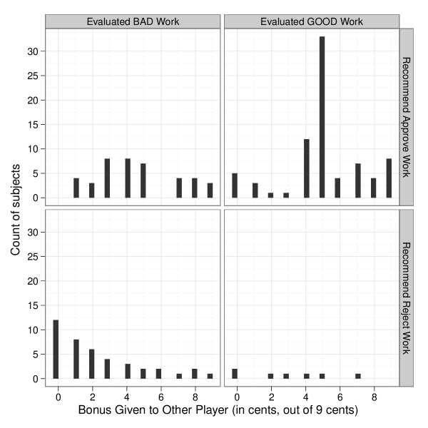
Figure 4: Experiment B, bonus allocation by treatment group and accept/reject recommendation. Subjects in $BAD$ evaluated work with $1$ generic label, while subjects in $GOOD$ evaluated work with $12$ specific and appropriate labels.

4.1.1 Workers more likely to advocate no pay for low productivity work

Regressing an indicator for approval on the treatment indicator, we have:

$$approve=\underbrace{0.418}_{[0.064]}\cdot GOOD+\underbrace{0.500}_{[0.056]}$$ (3)

with $n=167$ and $R^{2}=0.21$. Confirming what was evident graphically, subjects in $GOOD$ were far more likely to recommend approval.

4.1.2 Workers rewarded good work with generous bonuses

Subjects were more generous to their highly productive peers. Regressing the amount transferred on the treatment indicator, we have:

$$bonus=\underbrace{1.442}_{[0.393]}\cdot GOOD+\underbrace{3.488}_{[0.298]}$$ (4)

with $n=167$ and $R^{2}=0.08$.

4.1.3 Highly productive workers less generous and more likely to advocate rejection

There is a strong negative correlation between a subject’s own productivity and their generosity in the dictator game:

$$bonus=\underbrace{-0.259}_{[0.066]}\cdot y+\underbrace{5.376}_{[0.365]}$$ (5)

with $n=167$ and $R^{2}=0.07$. The effect also appears strongly in the approval recommendation:

$$approve=\underbrace{-0.055}_{[0.011]}\cdot y+\underbrace{0.960}_{[0.049]}$$ (6)

with $n=167$ and $R^{2}=0.11$.

4.2 Discussion

The perceived quality of the evaluated work had a strong causal effect on measures of both punishment and generosity. Subjects who evaluated low-output work were far more likely to recommend rejection and transfer smaller amounts of money in the dictator game. The simplest explanation may be that workers believe that their evaluations themselves may be spot-checked, and thus it is reasonable for them to adopt whatever they believe would be the principal’s view. In other words, they reject poor work because they believe that the employer/requester is likely to be believe it is bad. What is less clear is why highly productive workers are more likely to reject work. There are at least three possible explanations:

• There are different “types” of workers, and highly productive types (measured by producing high output on the initial image-labeling task) have a taste for punishment.

• Workers idiosyncratically differ in the perception of the prevailing productivity norm, and these differences in norm perception determine both output choices and norm enforcement.

• Workers are inequity-averse (Fehr and Schmidt, 1999), and because they regard productivity as costly, they punish low effort workers and reward high effort workers as a way to equalize outcomes.

5 Experiment C: Productivity and punishment

By definition, one cannot experimentally manipulate “innate types.” However, if manipulations of productivity cause a change in willingness to punish, then the innate types hypothesis is untenable. To distinguish inequity aversion from norm enforcement, one would need a way of manipulating a worker’s experienced productivity without changing either their perceptions of the prevailing norm or their perceptions of each party’s payoffs. In the parlance of the treatment effects literature, the exclusion restriction would need to be satisfied while not creating any non-random attrition. Given our imperfect understanding of how workers make decisions about both labor supply and generosity, it is unlikely that the exclusion restriction can be credibly satisfied. Nevertheless, ruling out the innate types hypothesis is still worthwhile, which is the goal in Experiment C.

To illustrate the challenge of distinguishing among the hypotheses, consider the implications of using the setup of Experiment A to induce changes in labor supply. In Experiment A we were able to change output by altering the work sample shown to workers before they accepted the task. We did not measure follow-on output in a second image-labeling task in Experiment A nor did we have them evaluate others work, but if we had, at least two problems would arise. First, the manipulation would have an effect on both the intensive margin and the extensive margin. Second, subjects who quit in the first stage would not record their choices in the dictator game or their answer to the accept/reject question.

The fundamental problem is that any intervention that changes worker pre-uptake beliefs about the work required—and hence the labor supply on the extensive margin—is likely to create a missing data problem. For this reason, the intervention used in Experiment C changes worker productivity after subjects have already begun working. The design, as well as the failed pilots, will be discussed in detail, but the key point is that the intervention successfully manipulated output on the intensive margin and yet did not cause any across-group differences on the extensive margin (i.e., lead to differences in group composition). However, it likely did affect perceived deservingness or inequity, making it impossible to decide between the two hypotheses related to these concepts.

5.1 Pilot experiments

Prior to running Experiment C, two failed pilot experiments were conducted. In the first pilot, half of the subjects were assigned to work with an interface containing a hidden “bug” that introduced a $1.2$-second delay in the software execution after each label was added; those in the control faced no delay. This pilot failed because it did not generate a “first stage” of reduced output—although workers in the “slow” treatment took longer, they did not produce any less output. This outcome is consistent with other findings that workers on MTurk appear insensitive to small time differences (Horton and Chilton, 2010).

In the second pilot, subjects in the “slow” treatment received a pop-up box containing the text “Thank you! Three is probably enough.” after they had added a second label but before they added a third label. Although this treatment did have a large effect on worker productivity, other aspects of the design of the experiment generated little variation in generosity. The first problem was that in order to obtain a larger sample, the $LOW$ work sample from Experiment A was used, thereby compressing the productivity distribution (as in Experiment A). The second problem was that workers evaluated work with $3$ good labels. As a result, regardless of their treatment assignment, many subjects chose the pseudo-50-50 (i.e., chose either the 4 or 5 cent transfer) split and recommended approval, providing little useful variation in measurements of punishment and generosity.

5.2 Actual experiment

After the two failed pilots, the second pop-up notice experiment was relaunched, albeit with two modifications. The $HIGH$ $9$-label work sample from Experiment A served as the sample, and the evaluated work was particularly bad—the evaluated worker provided only $1$ generic label for an item-rich photograph. Subjects were assigned to either $NONE$, in which they were given no notice, or $CURB$, in which they received the pop-up notice after completing a second label. Because two-stage least squares would be used in the data analysis, the total sample size was increased to $300$. Payment was 30 cents. Table 4 reports the summary statistics for experiment.

Table 4: Experiment C summary statistics ($n=273$)

Administrative
Launch: Sun Apr 18 19:36:44 GMT 2010
Finish: Wed Apr 21 05:18:02 GMT 2010
Survey	FALSE	TRUE	% TRUE
male	117	156	57.1
from India	175	98	35.9
from US	162	111	40.7
motivated by money	80	193	70.7
Treatment Assignment
$CURB=1$	133	140	51.3
Recommended we approve work?
in CURB	46	94	67.1
in NONE	57	76	57.1
Labels produced ($y$)	Min	.25	Med.	Mean	.75	Max
in CURB	1	2	3	2.979	4	10
in NONE	1	1	5	6.15	9	26
Bonus to evaluated worker
in CURB	0	2	4	3.871	5	9
in NONE	0	1	3	3.075	5	9

Notes: Overlap in subjects across experiments was $|C\cap B|=20$, $|C\cap A\cap\overline{B}|=20$. Subjects in $CURB$ reduced an output-reducing notification after adding a second label. The key results from the experiment can be seen in the mean differences across groups (in the “Bonus to evaluated worker” rows and the “Labels produced” rows).

5.3 Results

Worker output at the image-labeling task is binned and then plotted as two bar charts in Figure 5. The top panel shows the bar chart for subjects in $NONE$, while the bottom shows $CURB$. The bars themselves are filled in with the proportion of subjects in that band/group recommending rejection or acceptance of the evaluated work. Several features of the data are readily apparent. First, assignment to $CURB$ dramatically reduced output: a large numbers of subjects in $NONE$ produced $y\in(5,10]$ or $y\in(10,30]$. By comparison, less than $10$ subjects total in $CURB$ produced this much. Second, subjects choosing high levels of productivity in $NONE$, they were far more likely to recommend rejection. Although bonus allocation is not shown in the figure, this same pattern appears—subjects with reduced productivity (those in $CURB$) were more generous in their allocation of the $9$ cents.

5.3.1 Workers with reduced output more generous

There is a strong negative correlation between the amount transferred to the other player in the dictator game and a subject’s own output in the image-labeling task, as shown by:

$$bonus=\underbrace{-0.207}_{[0.039]}\cdot y+\underbrace{4.418}_{[0.223]}$$ (7)

with $n=273$ and $R^{2}=0.12$. Assignment to $CURB$ had a strong, negative effect on worker output, as shown by:

$$y=\underbrace{-3.172}_{[0.490]}\cdot CURB+\underbrace{6.150}_{[0.470]}$$ (8)

with $n=273$ and $R^{2}=0.14$. The F-statistic for the model is 43.982. The two-stage least squares estimate of the effect of output on transfers in the dictator game is:

$$bonus=\underbrace{-0.251}_{[0.090]}\cdot y+\underbrace{4.619}_{[0.433]}$$ (9)

There is no detectable difference between the OLS estimate of the effect of productivity on bonuses and the two stage least-squares estimate.

5.3.2 Workers with reduced output less likely to punish

As in Experiment B, highly productive subjects were more likely to recommend that we not approve the evaluated workers’ work:

$$approve=\underbrace{-0.042}_{[0.005]}\cdot y+\underbrace{0.811}_{[0.037]}$$ (10)

with $n=273$ and $R^{2}=0.13$. The two-stage least squares estimate is:

$$approve=\underbrace{-0.032}_{[0.017]}\cdot y+\underbrace{0.765}_{[0.083]}$$ (11)

which is not significantly different from the least-squares estimate.

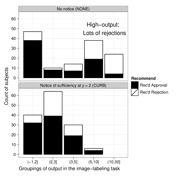
Figure 5: Output and punishment in Experiment C. This bar chart shows the amount of output in different output bands and the percentage of subjects in that band recommending approval or rejection. Note that a disproportionate number of subjects not receiving the output-curtailing message (subjects in $NONE$) produced relatively high levels of output and that subjects in that high-output band were much more likely to recommend rejection than low-output subjects.

5.4 Discussion

Experiment C rules out the possibility that productivity and generosity are jointly determined by some innate worker “type”: reducing productivity reduced willingness to punish. However, the experiment does not distinguish between the “enforced norms” hypothesis and the “inequity aversion” hypothesis. The problem stems in part from the difficulty in manipulating worker productivity without also altering workers’ perception of the relevant norm. It seems possible that future research could disentangle these hypothesis with a suitable experimental design.

However, other experimental results probably push the balance of evidence towards the enforced norms hypothesis. First, more complex laboratory games such as those conducted by Charness and Rabin (2002) show that workers trade off a number of competing interests when making dictator game allocations and that preferences are more nuanced than simple inequity aversion. List and Cherry (2008) make a compelling argument that what we often interpret as “social preferences” in the dictator game is in fact a desire to be seen as complying with some context-specific norm.

6 Experiment D: Peer effects from evaluation

Experiment A showed that exposure to employer-provided work samples affected labor supply, presumably by changing worker beliefs about the employer output expectations. Experiment D tested whether work samples from peers that are not held up as examples can still influence productivity. In set-up, Experiment D was similar to Experiment B in that after an initial task, subjects were assigned to one of two groups, $GOOD$ and $BAD$. In $GOOD$, subjects evaluated a worker that produced 11 labels; in $BAD$, subjects evaluated a worker that produced only 2 labels. Unlike Experiment B, however, subjects performed an additional image-labeling task after the evaluation. Table 5 reports the summary statistics for the experiment. The requested sample size was $300$ and payment was 40 cents.

Table 5: Experiment D summary statistics ($n=275$)

Administrative
Launch: Fri Apr 23 18:37:56 GMT 2010
Finish: Wed Apr 28 12:30:17 GMT 2010
Survey	FALSE	TRUE	% TRUE
male	131	144	52.4
from India	177	98	35.6
from US	154	121	44
motivated by money	76	199	72.4
Treatment Assignment
$GOOD=1$	142	133	48.4
Labels produced	Min	.25	Med.	Mean	.75	Max
Initial output, before evaluation ($y_{1}$)
in GOOD	1	2	5	4.759	7	14
in BAD	1	2	5	4.768	7	15
Follow-on output, after evaluation ($y_{2}$)
in GOOD	0	4	7	7.368	10	23
in BAD	0	1.25	5	5.014	7	16

Notes: Overlap in subjects across experiments was $|D\cap C|=26$, $|D\cap(A\cup B)\cap\overline{C}|=37$. Subjects in $GOOD$ evaluated high-output work, while subjects in $BAD$ evaluated low-output work. The key finding from this experiment was the effect exposure had on subsequent output. We can see that there were no differences in output means pre-exposure (“Initial output, before evaluation” rows) but a large difference after evaluation (“Follow-on output, after evaluation” rows).

6.1 Results

Exposure to the work of a peer strongly affected a subject’s subsequent output. Output following exposure to highly productive peers was higher than output following exposure to less productive peers. The treatment effect is heterogeneous across productivity distribution for the first task: more productive workers are more strongly affected by the exposure to peers.

Most of the results can be readily seen in Figure 6, which shows scatter plots of final output, $y_{2}$, against initial output, $y_{1}$. Observations from $BAD$ are represented in the plot by a “+” symbol and those in $GOOD$ by a “o” symbol. The two panels contain the scatter plot and regression line for the respective experimental group, as well as the points from the other group, lightly plotted. Because only integer-level outputs were possible, all points are randomly perturbed to prevent over-plotting. In the figure, the line for $GOOD$ is both above and steeper than the regression line for $BAD$, indicating non-constant effects.

6.1.1 Exposure to highly productive peers increased productivity

Subjects that evaluated highly productive work produced considerably more labels in the follow-on task:

$$y_{2}=\underbrace{0.914}_{[0.071]}\cdot y_{1}+\underbrace{2.362}_{[0.373]}\cdot GOOD+\underbrace{0.654}_{[0.398]}$$ (12)

with $n=275$ and $R^{2}=0.49$. In addition to the treatment effect, we can see that initial output was highly correlated with subsequent output. The effect of $GOOD$ was not, however, constant across the initial output distribution:

$$y_{2}=\underbrace{0.771}_{[0.073]}\cdot y_{1}+\underbrace{0.317}_{[0.142]}\cdot y_{1}GOOD+\underbrace{0.850}_{[0.799]}\cdot GOOD+\underbrace{1.337}_{[0.411]}$$ (13)

with $n=275$ and $R^{2}=0.5$; as $y_{1}$ increases, the positive effect of assignment to $GOOD$ on output grows larger.

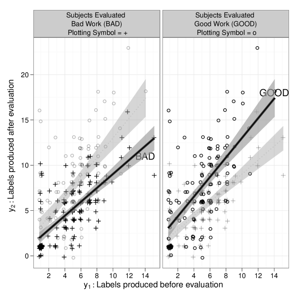
Figure 6: Subsequent output ($y_{2}$) versus initial output ($y_{1}$), by treatment group. All subjects did an identical initial task and chose some number of labels to provide (shown on the x-axis). Subjects then evaluated another subject’s work that demonstrated either low productivity ($BAD$, left panel) or high productivity ($GOOD$, right panel). All points from each group are shown in each panel (as well as the regression line), but the points and lines are either black or gray depending on whether they came from the experiment group shown in the panel. All output levels are randomly perturbed by $\epsilon\sim U[-.2,.2]$ to prevent over-plotting (which would occur because only integer output levels were possible).

6.2 Discussion

The peer effects detected in Experiment D strongly depend upon a worker’s initial output. There is no immediately obvious reason why this should be the case, however, studies from other domains have also found that different types of workers respond differently to peers. One possible explanation for the pattern is that initially less productive workers might already have strong beliefs that low productivity is acceptable. Recall that subjects were exposed to the $HIGH$ work sample from Experiment A prior to accepting the task, and yet still chose to produce only $1$ or $2$ labels. Although being in $GOOD$ and observing highly productive work might still have some effect on their beliefs, these less productive workers might have fairly stiff priors regarding what constitutes acceptable work.

Although Experiment D demonstrated that exposure to peer output affects a worker’s own output, it did not explain why workers are influenced by peers. There are several possible explanations for why peer effects exist in this setting including fear of punishment, learning about relevant employer standards and perhaps even an innate desire to match the performance of peers, regardless of the direct material payoff.

7 Experiment E: Peer effects after explicit employer instructions

Experiment D demonstrated the existence of productivity peer effects—even with the minimal “interaction” created by evaluation, yet it did not explain why workers are affected by peers. If peer effects reflect learning about employer standards, then clear, strongly stated production standards should “inoculate” workers from learning-driven peer effects. However, if workers fear punishment by fellow workers or if they have some innate desire to produce as much as peers, then we should detect peer effects even when standards are clearly communicated.

In Experiment E, these ideas were tested by providing subjects with very explicit instructions about productivity expectations and then exposing subjects to peers. The set-up was almost identical to that of Experiment D, except that workers were told that they should produce 2 and only 2 labels per image. The requirement of 2 labels was stated before workers began the task, and was repeated again with each of the two image-labeling tasks, directly above the image. After performing the initial task, workers were assigned to one of two groups: $OK$, in which subjects evaluated a work sample showing $y=2$, and $OVER$, in which subjects evaluated a work sample showing $y=11$. After evaluating the work, subjects performed an additional image-labeling task. Table 6 shows the summary statistics for the experiment. The requested sample size was $300$ and the payment was 40 cents.

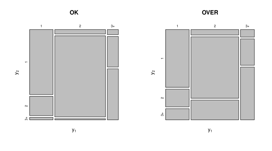
Figure 7: Mosaic plots showing the relationship between output in the initial task ($y_{1}$) to output in the follow-on task ($y_{2}$). In Experiment E, all subjects were told to produce $2$ and only $2$ labels. Subjects in $OK$ then evaluated work showing $2$ labels (hence complying with employer expectations), while subjects in $OVER$ evaluated work with $11$ labels. In both plots, the unit square is split vertically in thirds, in proportion to the number of subjects that selected $y_{1}=1$, $y_{1}=2$ and $y_{1}\geq 3$, respectively. Both plots are also split horizontally, in proportion to the number of subjects choosing $y_{2}=1$, $y_{2}=2$ and $y_{2}\geq 3$, respectively. The $(y_{1}=2,y_{2}=2)$ block in $OK$ is taller than the corresponding block in $OVER$, indicating that exposure to the complying work sample (in $OK$) made initially complying workers (i.e., those choosing $y_{1}=2$) more likely to comply in the follow on task (i.e., choosing $y_{2}=2$).

Table 6: Experiment E summary statistics ($n=272$)

Administrative
Launch: Wed May 19 21:19:42 GMT 2010
Finish: Sun May 23 15:26:30 GMT 2010
Survey	FALSE	TRUE	% TRUE
male	121	151	55.5
from India	136	136	50
from US	172	100	36.8
motivated by money	62	210	77.2
Treatment Assignment
$OK=1$	141	131	48.2
Labels produced	Min	.25	Med.	Mean	.75	Max
Initial output, before evaluation ($y_{1}$)
in OK	1	1	2	2.038	2	8
in OVER	1	1	2	2.085	2	8
Follow-on output, after evaluation ($y_{2}$)
in OK	1	2	2	1.977	2	8
in OVER	1	2	2	2.667	3	14

Notes: Overlap in subjects across experiments was $|E\cap D|=29$, $|E\cap(A\cup B\cup C)\cap\overline{D}|=42$. All subjects received explicit instructions to produce 2 labels. After performing one task, subjects were assigned to $OK$, where they viewed complying work, or $OVER$, where they viewed high-output/non-complying work. The key finding from the experiment can be seen in difference in group means in the “Follow on output, after evaluation” rows.

7.1 Results

The main results of Experiment E are readily apparent graphically, but the appropriate visualization is somewhat more complex. We would like to see how the choice of $y_{2}$ depended on $y_{1}$ and the assignment to $OK$ or $OVER$. Unfortunately, a scatter plot would be hard to interpret, as we expect many subjects to choose $y_{1}=2$ and $y_{2}=2$, per the instructions. Much information would be lost to over-plotting. A solution is to use a mosaic plot, which is useful for displaying relationships between categorical data.

In Figure 7, the left panel shows a mosaic plot for $OVER$, while the right panel shows same plot but for $OK$. Each pair-wise combination of output levels is represented by a rectangle. Output levels are top-censored, creating three output groups: $y=1$, $y=2$ and $y\geq 3$ (with $3+$ as a label for the final group). The width of each rectangle is proportional to the share of subjects that chose that respective level of output for $y_{1}$; the height on each rectangle is proportional to the number of subjects that chose that level of output for $y_{2}$.

Across both groups, most subjects chose $y_{1}=2$, suggesting that employer instructions to produce exactly 2 labels were salient. For subjects that complied initially, exposure to $OK$ was associated with a high level of compliance on the second task: only a tiny number of subjects increased or decreased output, as indicated by the very short $(y_{1}=2,y_{2}=1)$ and $(y_{1}=2,y_{2}=3+)$ rectangles. However, in $OVER$, many subjects that chose $y_{1}=2$ subsequently increased their output level after evaluating the $11$ label image, as seen by the tall rectangles associated with $y_{2}=3+$ in $OVER$.

7.1.1 Most workers compliant with employer output requests

In both $OVER$ and $OK$, we can see that $y_{1}=2$ was by far the most common output choice. Reassuringly, Figure 7 shows that the breakdown of $y_{1}$ appears almost identical across the two treatments. This is expected since subjects were randomized and the experience of the groups did not differ until after the first task was completed. The instruction to produce only two labels appears salient, especially considering the first stage was identical to that of this experiment that in Experiment A, $LOW$ (Figure 2, bottom panel), except that no explicit instructions were given, and in the Experiment A case, $y=2$ was not the modal choice, as it was in Experiment E.

7.1.2 Language barriers likely prevented full initial compliance

Although not causal, a regression of the compliance indicator on self-reported country suggests that language barriers might have limited compliance, with subjects from India significantly less likely to comply:

$$1\{y_{2}=2\}=\underbrace{-0.228}_{[0.059]}\cdot INDIA+\underbrace{0.691}_{[0.040]}$$ (14)

with $n=272$ and $R^{2}=0.05$.

7.1.3 Evaluating compliant work increased compliance for initially complying workers

Being assigned to $OK$ strongly increased $y_{2}$-compliance:

$$1\{y_{2}=2\}=\underbrace{0.161}_{[0.059]}\cdot OK+\underbrace{0.504}_{[0.042]}$$ (15)

with $n=272$ and $R^{2}=0.03$. This effect is driven by subjects in $OK$ who initially complied and then continued to comply on the second image. This is evidenced by the large and significant coefficient on the compliance $\times$ assignment interaction:

$$1\{y_{2}=2\}=\underbrace{0.022}_{[0.083]}\cdot OK+\underbrace{0.205}_{[0.102]}\cdot\left[OK\times 1\{y_{1}=2\}\right]+\underbrace{0.467}_{[0.076]}\cdot 1\{y_{1}=2\}+\underbrace{0.242}_{[0.055]}$$ (16)

with $n=272$ and $R^{2}=0.36$. Note that exposure to $OK$ has no effect for originally non-complying workers who chose $y_{1}\neq 2$. Also note that initial compliance was strongly predictive of subsequent compliance.

7.1.4 Workers did not punish non-complying work that demonstrated high effort

Assignment to $OK$ had no effect on subjects’ accept/reject recommendations:

$$approve=\underbrace{-0.002}_{[0.041]}\cdot OK+\underbrace{0.872}_{[0.028]}$$ (17)

with $n=272$ and $R^{2}=0$. For transfers in the dictator game:

$$bonus=\underbrace{-0.397}_{[0.263]}\cdot OK+\underbrace{5.305}_{[0.182]}$$ (18)

with $n=272$ and $R^{2}=0.01$. Note that the bonus level itself was quite high, and most subjects transferred a more than equitable split. Given the strong positive correlation between subjects’ own productivity and self-serving behavior in the dictator game, the large average bonus size is consistent with the fact that most subjects showed low productivity on the initial task (because they were induced to choose $y_{1}=2$). Although the coefficient on $OK$ in the regression above is not significant, it is not a precisely estimated zero, as in the case of approval in Equation 17. Self-serving behavior among subjects assigned to $OK$ is concentrated among highly productive types evaluating the $2$-label evaluated work. We can see this by the large negative coefficient on the group/productivity ($y_{1}\times OK$) interaction term:

$$bonus=\underbrace{0.720}_{[0.502]}\cdot OK+\underbrace{0.020}_{[0.152]}\cdot y_{1}+\underbrace{-0.547}_{[0.204]}\cdot y_{1}\times OK+\underbrace{5.264}_{[0.383]}$$ (19)

with $n=272$ and $R^{2}=0.05$.

7.1.5 Exposure to highly productive work increased output even when expectations were explicit

Workers exposed to $OVER$ increased their output compared to those exposed to $OK$:

$$y_{2}=\underbrace{0.658}_{[0.120]}\cdot y_{1}+\underbrace{-0.659}_{[0.183]}\cdot OK+\underbrace{1.294}_{[0.299]}$$ (20)

with $n=272$ and $R^{2}=0.25$. However, unlike in Experiment D, this effect was not conditional upon initial output. When the regression above is augmented with an $y_{1}\cdot OK$ interaction term (not shown), the coefficient on the interaction is small and insignificant, which is consistent with there being little variation in initial output (i.e., the distribution of $y_{1}$ is heavily concentrated at $y_{1}=2$).

7.2 Discussion

It is clear that many workers take explicit requests from employers as informative and worth complying with. Yet a substantial number of workers remained susceptible to peer effects that could, in principle, have led them to have their work rejected for not following the letter of the instructions. There are several possible explanations.

One possibility is mistake. Workers might believe that they misinterpreted the instructions or that other workers have some inside knowledge. Workers might reasonably believe that we had free disposal of extra labels and added a few more to provide a margin of safety. However, the requirement was clearly stated at least three times to workers, and many initially complying workers were still pulled upward by highly productive peers.

Another possibility is that workers want to produce an amount comparable to that of their peers, regardless of employer instructions. Given the propensity of peers to punish low effort, matching the output of one’s peers is a good idea if there is a chance one will be evaluated by those peers. Because subjects are asked to evaluate workers, it seems likely that they infer they will also be evaluated by other workers. Given that other workers are likely to reward or punish based on apparent effort, not necessarily on compliance with the stated standards, above-standard output could be rational even if it is technically non-complying.

8 Conclusion

This paper reports a number of results on punishment, productivity and peer effects: (1) workers readily punish low-effort work; (2) workers are susceptible to peer effects, but the effects are conditional upon a worker’s productivity; (3) a worker’s willing to punish is mediated by their own productivity, which is in turn malleable; (4) workers punish low effort, not failure to comply with an employer’s instructions. Some of these findings contradict or at least complicate results from other workplace settings. Future research should investigate the generalizability of these findings and which should clarify which findings are general features of how humans think about work and which are context-specific.

If strong reciprocity is a general feature of human organizations, then a natural question for managers is whether they should encourage this phenomenon among workers. Here, context seems to matter greatly. Giving workers thicker sticks or juicier carrots to use on their peers may backfire if workers are enforcing norms contrary to the best interests of the firm. Further, other research has shown that workers will enforce norms that are directly counter productive (e.g., Roy’s 1952 work on machine shops). Creating the tools for norm enforcement is risky when knowledge of what will be enforced is murky.

A key theme of these experiments is the apparent pliability of productivity, which highlights the danger of what might be called “organizational alchemy,” i.e., the attempt to harness the power of peer effects without knowing how they work in the relevant context. For example, in contrast to several other findings, “bad” workers did not improve after evaluating good work. At least in the context examined, it would be a mistake to mix workers of different abilities with the hope that the good would raise the bad.

References

- (1)
- Bandiera et al. (2010) Bandiera, O., I. Barankay, and I. Rasul, “Social incentives in the workplace,” Review of Economic Studies, 2010, 77 (2), 417–458.
- Carpenter et al. (2009) Carpenter, J., S. Bowles, H. Gintis, and S.H. Hwang, “Strong reciprocity and team production: Theory and evidence,” Journal of Economic Behavior & Organization, 2009, 71 (2), 221–232.
- Chandler and Kapelner (2010) Chandler, D. and A. Kapelner, “Breaking monotony with meaning: Motivation in crowdsourcing markets,” University of Chicago mimeo, 2010.
- Charness and Rabin (2002) Charness, G. and M. Rabin, “Understanding social preferences with simple tests,” Quarterly Journal of Economics, 2002, 117 (3), 817–869.
- Engel (2010) Engel, C., “Dictator games: A meta study,” Working Paper Series of the Max Planck Institute for Research on Collective Goods, 2010.
- Falk and Ichino (2006) Falk, A. and A. Ichino, “Clean evidence on peer effects,” Journal of Labor Economics, 2006, 24 (1).
- Fehr and Schmidt (1999) Fehr, E. and K.M. Schmidt, “A theory of fairness, competition, and cooperation,” Quarterly Journal of Economics, 1999, 114 (3), 817–868.
- Fehr and Gachter (2000) and S. Gachter, “Cooperation and punishment in public goods experiments,” American Economic Review, 2000, pp. 980–994.
- Fehr and Gachter (2002) and , “Altruistic punishment in humans,” Nature, 2002, 415 (6868), 137–140.
- Frei (2009) Frei, Brent, “Paid crowdsourcing: Current state & progress toward mainstream business use,” Whitepaper Produced by Smartsheet.com, 2009.
- Guryan et al. (2009) Guryan, J., K. Kroft, and M.J. Notowidigdo, “Peer effects in the workplace: Evidence from random groupings in professional golf tournaments,” American Economic Journal: Applied Economics, 2009, 1 (4), 34–68.
- Harrison and List (2004) Harrison, G.W. and J.A. List, “Field experiments,” Journal of Economic Literature, 2004, 42 (4), 1009–1055.
- Holmstrom (1982) Holmstrom, B., “Moral hazard in teams,” The Bell Journal of Economics, 1982, 13 (2), 324–340.
- Horton (2010a) Horton, J.J., “Online Labor Markets,” Working Paper, 2010.
- Horton (2010b) , “The Condition of the Turking class: Are Online Employers Fair and Honest?,” Arxiv preprint arXiv, 2010, 1001.
- Horton and Chilton (2010) and L.B. Chilton, “The labor economics of paid crowdsourcing,” in “Proceedings of the 11th ACM Conference on Electronic Commerce” 2010.
- Horton et al. (2010) , D.G. Rand, and R. J. Zeckhauser, “The online laboratory: Conducting experiments in a real labor market,” NBER Working Paper w15961, 2010.
- Huang et al. (2010) Huang, E., H. Zhang, D.C. Parkes, K.Z. Gajos, and Y. Chen, “Toward automatic task design: A progress report,” in “Proceedings of the ACM SIGKDD Workshop on Human Computation (HCOMP)” 2010.
- Ipeirotis (2010) Ipeirotis, P.G., “Demographics of Mechanical Turk,” New York University Working Paper, 2010.
- Ipeirotis et al. (2010) , F. Provost, and J. Wang, “Quality Management on Amazon Mechanical Turk,” in “Proc. ACM SIGKDD Workshop on Human Computation (HCOMP)” 2010.
- Katz (1986) Katz, L.F., “Efficiency wage theories: A partial evaluation,” NBER macroeconomics annual, 1986, 1, 235–276.
- Levin (2003) Levin, J., “Relational incentive contracts,” American Economic Review, 2003, 93 (3), 835–857.
- List and Cherry (2008) List, J.A. and T.L. Cherry, “Examining the role of fairness in high stakes allocation decisions,” Journal of Economic Behavior & Organization, 2008, 65 (1), 1–8.
- Little et al. (2010) Little, G., L.B. Chilton, , M. Goldman, and R. Miller, “Exploring iterative and parallel human computation processes,” in “ACM-KDD (HCOMP)” ACM 2010.
- Manski (1993) Manski, C.F., “Identification of endogenous social effects: The reflection problem,” The Review of Economic Studies, 1993, 60 (3), 531–542.
- Mas and Moretti (2009) Mas, A. and E. Moretti, “Peers at work,” American Economic Review, 2009, 99 (1), 112–145.
- Mason and Watts (2009) Mason, W. and D.J. Watts, “Financial incentives and the ‘performance of crowds’,” in “Proc. ACM SIGKDD Workshop on Human Computation (HCOMP)” 2009.
- Roy (1952) Roy, D., “Quota restriction and goldbricking in a machine shop,” American Journal of Sociology, 1952, 57 (5), 427–442.
- Schein (2004) Schein, E.H., Organizational culture and leadership, Jossey-Bass Inc Pub, 2004.
- von Ahn and Dabbish (2004) von Ahn, L. and L. Dabbish, “Labeling images with a computer game,” in “Proceedings of the ACM SIGCHI conference on Human factors in computing systems” 2004, pp. 319–326.
- Wickham (2008) Wickham, H., “ggplot2: An implementation of the grammar of graphics,” R package version 0.7, URL: http://CRAN.R-project.org/package=ggplot2, 2008.