Does a low solar cycle minimum hint at a weak upcoming cycle?

Abstract

The maximum amplitude ($R_{\mathrm{m}}$) of a solar cycle, in the term of mean sunspot numbers, is well-known to be positively correlated with the preceding minimum ($R_{\mathrm{min}}$). So far as the long term trend is concerned, a low level of $R_{\mathrm{min}}$ tends to be followed by a weak $R_{\mathrm{m}}$, and vice versa. In this paper, we found that the evidence is insufficient to infer a very weak Cycle 24 from the very low $R_{\mathrm{min}}$ in the preceding cycle. This is concluded by analyzing the correlation in the temporal variations of parameters for two successive cycles.

1 Introduction

Studying the correlation between the maximum amplitude ($R_{\mathrm{m}}$) of a solar cycle and the preceding minimum ($R_{\mathrm{min}}$) is useful for understanding the long-term evolution of solar activity. This can provide information about the activity level of an ensuing cycle. The positive correlation between $R_{\mathrm{m}}$ and $R_{\mathrm{min}}$ is a well-known fact (Hathaway et al., 2002). As a natural consequence, the very low level of solar activity at the present time (around the onset of Cycle 24) seems to be followed by a very weak (Svalgaard et al., 2005; Schatten, 2005), or even the weakest cycle (Li, 2009). However, a lower $R_{\mathrm{min}}$ has not always been followed by a weaker cycle. For example, a small $R_{\mathrm{min}}$ precedes the greatest $R_{\mathrm{m}}$ in Cycle 19 (Wang & Sheeley, 2009). Therefore, what information we can infer from the preceding minimum is worth re-analyzing carefully. We ask whether and how past cycles affect the present cycle.

A more accurate prediction of solar activity is an important task in solar physics and space weather. Knowing in advance the activity level of an upcoming cycle is helpful in the launching and operation of spacecrafts. An underestimate of the activity level for the next cycle may let down our guard. One aim of this study serves to remind the space flight mission planners that they still need to remain vigilant to avoid unexpected troubles.

In the present study, we use the 13-month running mean of Zürich relative sunspot number from January 1749 to April 2010 to determine the maximum ($R_{\mathrm{m}}$) and the preceding minimum ($R_{\mathrm{min}}$) of the solar cycle. The correlation between $R_{\mathrm{m}}$ and $R_{\mathrm{min}}$ for different periods of time is shown in Section 2. In Section 3, we examine the varying trends of $R_{\mathrm{m}}$ and $R_{\mathrm{min}}$ using a quantity to describe whether a parameter increases or decreases. Then, in Section 4, we analyze the temporal variation in the correlation coefficient between $R_{\mathrm{m}}$ and $R_{\mathrm{min}}$ with a moving time window of five cycles. The results are briefly discussed and summarized in Section 5.

2 Correlation between $R_{\mathrm{m}}$ and $R_{\mathrm{min}}$

The parameters of $R_{\rm m}$ and $R_{\rm min}$ since cycle $n=1$ are listed in Table 1, and shown in Fig. 1a.

Figure 1: (a) $R_{\mathrm{m}}$(solid) and $R_{\mathrm{min}}$(dotted) since cycle $n=1$. (b) Scatter plot of $R_{\mathrm{m}}$ against $R_{\mathrm{min}}$ (triangles). (c) Varying trend: $V_{\mathrm{m}}$(solid) and $V_{\mathrm{min}}$(dotted).

It can be seen from Fig. 1a that $R_{\mathrm{m}}$ and $R_{\mathrm{min}}$ have a similar long-term variation behavior: a lower (higher) level of $R_{\mathrm{min}}$ tends to be followed by a weaker (stronger) $R_{\mathrm{m}}$. Their correlation coefficient is $r=0.56$ at a confidence level (CL) of 99%. The scatter plot of $R_{\mathrm{m}}$ against $R_{\mathrm{min}}$ (triangles) is shown in Fig. 1b. Their least-squares-fit linear regression equation is:

$$R_{\mathrm{m}}=77.9+5.98R_{\mathrm{min}},\quad\sigma=33.5,$$ (1)

where $\sigma$ is the standard deviation of the equation. Substituting the present value of $R_{\mathrm{min}}$ (1.7) into this equation, the peak of Cycle 24 is predicted as $R_{\mathrm{m}}(24)=88.0\pm 33.5$ (labeled by a star), regarding the 1-$\sigma$ uncertainty. When using the modern era data since Cycle 10, the peak of Cycle 24 is predicted to be higher, as $R_{\mathrm{m}}(24)=98.4\pm 35.0$. When using only the recent nine cycles since Cycle 15, an even higher value of $R_{\mathrm{m}}(24)=122.3\pm 36.5$ will be predicted for Cycle 24.

However, Li (2009) inferred a rather low level for Cycle 24, $R_{\mathrm{m}}(24)=58.0\pm 26.6$, from a relationship of $R_{\mathrm{m}}=48.8+5.39R_{\mathrm{min}}\pm 26.6$ derived by Hathaway et al. (2002). The data used to derive this relationship are those that are smoothed with the 24-month Gaussian filter, rather than the ’standard’ 13-month running mean. So, the present minimum value ($R_{\mathrm{min}}=1.7$) of the 13-month running mean sunspot number is inappropriate for use in inferring an $R_{\mathrm{m}}(24)$ value from this relationship. Besides, the $R_{\mathrm{min}}$ value in terms of the 24-month Gaussian filter is unknown within 12 months of the minimum. (Even if this value is known, the result inferred from the above relationship has a different meaning.)

We return to Fig. 1a. If using only the parameters in the earlier cycles of $n=1$–14 (left to the vertical line in Fig. 1a), the correlation coefficient between $R_{\mathrm{m}}$ and $R_{\mathrm{min}}$ increases to $r(1$-14$)=0.72$ at the 99% level of confidence. In contrast, for the recent cycles of $n=15$–23, the correlation coefficient is only $r($15-$23)=0.23$, which is statistically insignificant (CL $<50\%)$. Therefore, the positive correlation between $R_{\mathrm{m}}$ and $R_{\mathrm{min}}$ (0.56) is mostly contributed by the earlier cycles. The recent cycles, especially for cycles 15–19, seem to behave differently from the earlier cycles. It is then necessary to analyze whether the temporal variation in the correlation affects the future $R_{\mathrm{m}}$ value.

3 Trends of variations in $R_{\mathrm{m}}$ and $R_{\mathrm{min}}$

It should be noted in Fig. 1a that, for an individual cycle, the increase or decrease of $R_{\mathrm{m}}$ does not always follow that of $R_{\mathrm{min}}$. For example, $R_{\mathrm{min}}$ decreases while $R_{\mathrm{m}}$ increases from $n=18$ to 19. To demonstrate the behavior of increasing or decreasing, we define the varying trends of $R_{\mathrm{m}}$ and $R_{\mathrm{min}}$ as:

$$\begin{array}[]{lll}V_{\mathrm{m}}(n)&=&\mathrm{Sgn}(R_{\mathrm{m}}(n)-R_{\mathrm{m}}(n-1)),\\ V_{\mathrm{min}}(n)&=&\mathrm{Sgn}(R_{\mathrm{min}}(n)-R_{\mathrm{min}}(n-1)),\end{array}$$ (2)

where $y=\mathrm{Sgn}(x)$ is the sign function: $y=1$ if $x>0$, $y=-1$ if $x<0$ and $y=0$ if $x=0$. $V_{\mathrm{m}}(n)=+1$ refers to an increase in $R_{\mathrm{m}}(n)>R_{\mathrm{m}}(n-1)$, and $V_{\mathrm{m}}(n)=-1$ refers to a decrease in $R_{\mathrm{m}}(n)<R_{\mathrm{m}}(n-1)$, and so on. $V_{\mathrm{m}}(n)=V_{\mathrm{min}}(n)$ refers to the same trend of $R_{\mathrm{m}}(n)$ and $R_{\mathrm{min}}(n)$. The values of $V_{\mathrm{m}}(n)$ and $V_{\mathrm{min}}(n)$ are listed in Table 1 and shown in Fig. 1c. For all cycles $n=2$–23, there are 13/9 pairs of $V_{\mathrm{m}}(n)$ and $V_{\mathrm{min}}(n)$ with the same/opposite trends. Their correlation is very weak, at $r=0.18$, and statistically insignificant (CL = 57%).

For the earlier cycles of $n=2$–14, there are 10/3 pairs of $V_{\mathrm{m}}(n)$ and $V_{\mathrm{min}}(n)$ with the same/opposite trends, and their correlation coefficient is $r_{V}(2$-$14)=0.55$ at the 95% level of confidence. In contrast, for the recent cycles of $n=15$–23, there are 3/6 pairs with the same/opposite trends, and their correlation coefficient becomes negative, at $r_{V}(2$-$14)=-0.35$, at the 63% level of confidence. If we consider only the case of $V_{\mathrm{min}}(n)=-1$, as for $n=3$, 5, 6, 10, 12, 14, 15, 17, 19, and 23, there are 6/4 pairs with the same/opposite trends. For the earlier cycles of $n\leq 14$, there are 5/1 pairs for $V_{\mathrm{min}}(n)=-1$ with the same/opposite trends, while for the recent cycles of $n\geq 15$, there are 1/3 pairs for $V_{\mathrm{min}}(n)=-1$ with the same/opposite trends. This implies that a decrease in $R_{\mathrm{min}}$ is indeed followed by a decrease in $R_{\mathrm{m}}$ in most of the earlier cycles, while in the recent cycles, a decrease of $R_{\mathrm{min}}$ tends to be followed by an increase of $R_{\mathrm{m}}$.

In summary, in terms of the varying trend, there is no statistically significant positive correlation between $V_{\mathrm{m}}$ and $V_{\mathrm{min}}$ for all cycles ($r=0.18$). The positive correlation between $V_{\mathrm{m}}$ and $V_{\mathrm{min}}$ exists only in the earlier cycles ($r_{V}(2$-$14)=0.55$) at the 95% level of confidence. Concerning in the recent cycles, this correlation becomes negative ($r_{V}(2$-$14)=-0.35$). The behavior of the varying trend changed in recent cycles. Therefore, we cannot infer a decrease of $R_{\mathrm{m}}$ from a decrease of $R_{\mathrm{min}}$ for Cycle 24.

4 Temporal Variation in the Running Correlation

In the previous two sections, one has noted that the correlation between $R_{\mathrm{m}}$ and $R_{\mathrm{min}}$ behaves differently for different periods of time. Now, we analyze the temporal variation in the running correlation with a moving time window of $w=5$ cycles. For each cycle $n$, we calculate the correlation coefficient between $R_{\mathrm{m}}(i)$ and $R_{\mathrm{min}}(i)$ for $i=n-2,n-1,\ldots,n+2$ (Du et al., 2009a), denoted by $r(5,n)$. The results are shown in Fig. 2a.

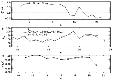
Figure 2: (a) Running correlation coefficient between $R_{\mathrm{m}}$ and $R_{\mathrm{min}}$ for a 5-cycle moving window. Stars indicate that the relevant values are significant at the 90% level of confidence. (b) $R_{\mathrm{m}}$ (solid) versa the fitted value (dotted) from Equation (3). (c) Running correlation coefficient of $R_{\mathrm{m}}$ with both $aa_{\mathrm{min}}$ and $R_{\mathrm{min}}$ for a 5-cycle moving window.

It can be seen that the correlation is positive before $n=13$ and significant at the 90% level of confidence for cycles $n=5$–9 (stars). This implies that a lower (higher) level of $R_{\mathrm{min}}$ tends to be followed by a weaker (stronger) $R_{\mathrm{m}}$ for these earlier cycles. However, the correlation decreases since $n=14$, and becomes negative since $n=18$, implying that a lower $R_{\mathrm{min}}$ corresponds to a stronger $R_{\mathrm{m}}$ (see also $n=15$, 17 and 19 in Fig. 1a). Therefore, a lower $R_{\mathrm{min}}$ has not always been followed by a weaker $R_{\mathrm{m}}$. In other words, we cannot infer a very weak $R_{\mathrm{m}}$ of Cycle 24 from the preceding very low level of $R_{\mathrm{min}}$.

5 Discussions and Conclusions

It is well known that the maximum amplitude ($R_{\mathrm{m}}$) of a solar cycle is positively correlated with the preceding minimum ($R_{\mathrm{min}}$), so that a low $R_{\mathrm{min}}$ tends to be followed by a weak $R_{\mathrm{m}}$. However, this relationship is not always effective for individual cycles (Wang & Sheeley, 2009), especially for the recent cycles, as shown in Fig. 2a. The correlation between $R_{\mathrm{m}}$ and $R_{\mathrm{min}}$ varies with time ($n$).

We analyzed the temporal behavior of this correlation and the varying trends ($V$) of $R_{\mathrm{m}}$ and $R_{\mathrm{min}}$. In the recent cycles, they all show a negative correlation. Since the prediction of $R_{\mathrm{m}}$ relies more on the recent cycle rather than on the past cycles (Schatten, 2005; Svalgaard et al., 2005; Du et al., 2008, 2009b), the negative correlation in the recent cycles cannot infer a very weak $R_{\mathrm{m}}$ from a very low $R_{\mathrm{min}}$.

One may argue that $R_{\mathrm{m}}$ and $R_{\mathrm{min}}$ have a similar shape in the most recent four cycles of $n=20$–23. Along with the developing trend of these cycles, $R_{\mathrm{m}}(24)$ should be very small. However, whether this behavior holds true is questionable before and after these cycles. It should be noted in Fig. 1a that $R_{\mathrm{m}}$ has never decreased in three successive cycles. The $R_{\mathrm{m}}$ value decreased two cycles from $n=3$ to 5, and then leveled off to $n=6$, and decreased two cycles from $n=8$ to 10, and then increased to $n=11$. Now that the $R_{\mathrm{m}}$ value decreased two cycles from $n=21$ to 23, it seems to increase or level off according to its past behavior. On the other hand, $R_{\mathrm{min}}(24)$ is not the lowest one ever seen. It is higher than cycles 6, 7 (Fig. 1a), and 15 (Li, 2009): $R_{\mathrm{min}}(24)>R_{\mathrm{min}}(15)>R_{\mathrm{min}}(7)>R_{\mathrm{min}}(6)$. However, corresponding to these local minima, the following $R_{\mathrm{m}}$ values are not local minima: $R_{\mathrm{m}}(6)\sim R_{\mathrm{m}}(5)$, $R_{\mathrm{m}}(7)>R_{\mathrm{m}}(6)$, and $R_{\mathrm{m}}(15)>R_{\mathrm{m}}(14)$. From this information, we cannot yet infer that Cycle 24 is a local minimum. To say the least, it is unlikely that Cycle 24 will be the weakest cycle.

In conclusion, we have not found sufficient evidence for the low(est) level of Solar Cycle 24 inferred from the low level of the present state. The sunspot number is highly correlated with other solar activity indices, such as sunspot group number, sunspot area, solar radio flux, and so on. Therefore, the above conclusions can also be reached when using these indices.

Near the time of the solar cycle minimum, geomagnetic activity is a much better indicator of the ensuing maximum amplitude ($R_{\mathrm{m}}$) for the sunspot cycle (Ohl, 1966) than the minimum amplitude is ($R_{\mathrm{min}}$). Hathaway et al. (1999; 2009) tested the predictive powers of several methods for cycles 19-23, and concluded that the geomagnetic-related precursor methods outperform the others. The minimum smoothed monthly mean aa index ($aa_{\mathrm{min}}$) near the time of the solar cycle minimum is shown in Table 1, in which the values of cycles 9-11 are taken from the equivalent annual values (Du et al., 2009b). One can note that the varying trend (V) of $R_{\mathrm{m}}$ follows well with that of $aa_{\mathrm{min}}$ — with only the two exceptions of cycles 16 and 22. The correlation coefficient between $R_{\mathrm{m}}$ and $aa_{\mathrm{min}}$ is usually as high as 0.9 (Du et al., 2009b). The application of $aa_{\mathrm{min}}$ in the prediction of $R_{\mathrm{m}}$ can be found, for example, in Hathaway (2009) and Du et al. (2009b). Wilson et al. (1998) suggested the bivariate of both $aa_{\mathrm{min}}$ and $R_{\mathrm{min}}$ to predict $R_{\mathrm{m}}$. Using the data for cycles 9-23 in Table 1, the bivariate-fit regression equation of $R_{\mathrm{m}}$ versus both $aa_{\mathrm{min}}$ and $R_{\mathrm{m}}$ is:

$$R_{\mathrm{m}}=5.0+10.56aa_{\mathrm{min}}-3.18R_{\mathrm{min}},\quad\sigma=15.3,$$ (3)

where $\sigma$ is the standard deviation of the equation. Figure  2b shows the observed $R_{\mathrm{m}}$ (solid) and the fitted $R_{\mathrm{m}}$ (dotted) from the above equation. Substituting the values of $aa_{\mathrm{min}}(8.4)$ and $R_{\mathrm{min}}$ (1.7) into this equation, the peak of the next cycle is predicted as $R_{\mathrm{m}}(24)=88.3\pm 15.3$ (labeled by a star). This prediction is close to that predicted by the single variate of $R_{\mathrm{min}}$ in Equation (1). But, the correlation for the bivariate of both $aa_{\mathrm{min}}$ and $R_{\mathrm{m}}(r=0.92)$ is much higher than that of the single variate of $R_{\mathrm{min}}(r=0.56)$. If this prediction comes true, Cycle 24 will be modest rather than the lowest one.

The prediction of $R_{\mathrm{m}}$ is related to the behavior of solar activity in the past cycles. Du et al. (2009b) pointed out that Ohl’s precursor method performed well only if the related correlation coefficient becomes stronger. If the correlation coefficient becomes weaker, its prediction would be questionable. Figure 2c shows the running correlation coefficient $r(5,n)$ of $R_{\mathrm{m}}$ with both $aa_{\mathrm{min}}$ and $R_{\mathrm{min}}$ for a five-cycle moving window. It is seen that the last value ($n=21$, corresponding to the data for cycles 19-23) drops drastically. Therefore, other methods are needed to check the above prediction.

Predicting the future level of a solar cycle is a complex project in solar physics and space weather (Wang et al., 2009). This paper stresses that the low level of $R_{\mathrm{min}}$ in the present state is insufficient to infer a low(est) level for Solar Cycle 24, as suggested by Li (2009). Whether a prediction from a simple parameter succeeds is related to the behavior of solar activity in the past few cycles. When a solar cycle is well underway (two to three years after the minimum), its behavior can be predicted to a good extent with curve fitting techniques (Hathaway, 2009).

Table 1: Cycle maximum ($R_{\rm m}$), minimum ($R_{\rm min}$) and minimum aa index ($aa_{\rm min}$) and their trends (V).

$n$	$R_{\rm m}(V)$	$R_{\rm min}(V)$	$aa_{\rm min}$	$n$	$R_{\rm m}(V)$	$R_{\rm min}(V)$	$aa_{\rm min}$
1	86.5	8.4		13	$87.9(+)$	$5.0(+)$	$10.6(+)$
2	$115.8(+)$	$11.2(+)$		14	$64.2(-)$	$2.7(-)$	$5.9(-)$
3	$158.5(+)$	$7.2(-)$		15	$105.4(+)$	$1.5(-)$	$8.2(+)$
4	$141.2(-)$	$9.5(+)$		16	$78.1(-)$	$5.6(+)$	$9.4(+)$
5	$49.2(-)$	$3.2(-)$		17	$119.2(+)$	$3.5(-)$	$13.2(+)$
6	$48.7(-)$	$0.0(-)$		18	$151.8(+)$	$7.7(+)$	$16.3(+)$
7	$71.5(+)$	$0.1(+)$		19	$201.3(+)$	$3.4(-)$	$16.9(+)$
8	$146.9(+)$	$7.3(+)$		20	$110.6(-)$	$9.6(+)$	$13.8(-)$
9	$131.9(-)$	$10.6(+)$	14.1	21	$164.5(+)$	$12.2(+)$	$17.2(+)$
10	$98.0(-)$	$3.2(-)$	$10.3(-)$	22	$158.5(-)$	$12.3(+)$	$17.5(+)$
11	$140.3(+)$	$5.2(+)$	$16.0(+)$	23	$120.8(-)$	$8.0(-)$	$15.9(-)$
12	$74.6(-)$	$2.2(-)$	$6.7(-)$	24	? (?)	$1.7(-)$	$8.4(-)$

References

- Du et al. (2008) Du, Z. L., Wang, H. N., & Zhang, L. Y. 2008, Chin. J. Astron. Astrophys. (ChJAA), 8, 477
- Du et al. (2009a) Du, Z. L., Wang, H. N., & Zhang, L. Y. 2009a, Sol. Phys., 255, 179
- Du et al. (2009b) Du, Z. L., Li, R., & Wang, H. N. 2009b, AJ, 138, 1998
- Hathaway et al. (1999) Hathaway, D. H., Wilson, R. M., & Reichmann, E. J. 1999, J. Geophys. Res., 104, 22,375
- Hathaway et al. (2002) Hathaway, D. H., Wilson, R. M., & Reichmann, E. J. 2002, Sol. Phys., 211, 357
- Hathaway (2009) Hathaway, D. H. 2009, Space Sci. Rev., 144, 401
- Li (2009) Li, K. J. 2009, Research in Astron. Astrophys. (RAA), 9, 959
- Ohl (1966) Ohl, A. I. 1966, Solice Danie, 9, 84
- Schatten (2005) Schatten, K. H. 2005, Geophys. Res. Lett., 32, L21106
- Svalgaard et al. (2005) Svalgaard, L., Cliver, E. W., & Kamide, Y. 2005, Geophys. Res. Lett., 32, 1104
- Wang & Sheeley (2009) Wang, Y. M., & Sheeley, N. R. 2009, ApJ, 694, L11
- Wang et al. (2009) Wang, J. L., et al. 2009, Research in Astron. Astrophys. (RAA), 9, 133
- Wilson et al. (1998) Wilson, R. M., Hathaway, D. H., & Reichmann, E. J. 1998, J. Geophys. Res., 103, 6595