Transit spectrophotometry of the exoplanet HD189733b.
II. New Spitzer observations at 3.6 $\mu$m

Abstract

Context. We present a new primary transit observation of the hot-jupiter HD 189733b, obtained at 3.6 $\mu$m with the Infrared Array Camera (IRAC) onboard the Spitzer Space Telescope. Previous measurements at 3.6 microns suffered from strong systematics and conclusions could hardly be obtained with confidence on the water detection by comparison of the 3.6 and 5.8 microns observations.

Aims. We aim at constraining the atmospheric structure and composition of the planet and improving over previously derived parameters.

Methods. We use a high-$S/N$ Spitzer photometric transit light curve to improve the precision of the near infrared radius of the planet at 3.6 $\mu$m. The observation has been performed using high-cadence time series integrated in the subarray mode. We are able to derive accurate system parameters, including planet-to-star radius ratio, impact parameter, scale of the system, and central time of the transit from the fits of the transit light curve. We compare the results with transmission spectroscopic models and with results from previous observations at the same wavelength.

Results. We obtained the following system parameters of $R_{p}/R_{\star}=0.15566^{+0.00011}_{-0.00024}$, $b=0.661^{+0.0053}_{-0.0050}$, and $a/R_{\star}=8.925^{+0.0490}_{-0.0523}$ at 3.6 $\mu$m. These measurements are three times more accurate than previous studies at this wavelength because they benefit from greater observational efficiency and less statistic and systematic errors. Nonetheless, we find that the radius ratio has to be corrected for stellar activity and present a method to do so using ground-based long-duration photometric follow-up in the V-band. The resulting planet-to-star radius ratio corrected for the stellar variability is in agreement with the previous measurement obtained in the same bandpass (Désert et al. 2009). We also discuss that water vapour could not be evidenced by comparison of the planetary radius measured at 3.6 and 5.8 $\mu$m, because the radius measured at 3.6 $\mu$m is affected by absorption by other species, possibly Rayleigh scattering by haze.

1 Introduction

HD 189733b is a transiting hot jupiter that orbits a small, bright, main-sequence K2V star ($K=5.5$) and produces deep transits of $\sim$2.5% (Bouchy et al. 2005). The planet has a mass of $M_{p}=1.13$ Jupiter mass (M_J), a radius of $R_{p}=1.16$ Jupiter radius (R_J) in the visible (Bakos et al. 2006b; Winn et al. 2007), and a brightness temperature ranging between 950 and 1220 K (Knutson et al. 2007). This implies a large atmospheric scale height (200 km), allowing transits to characterize the chemical composition and vertical structure of the atmosphere.

Transmission spectroscopy during transit allows the upper part of the atmosphere to be probed, down to altitudes where it becomes optically thick. Therefore, one can infer the composition of the atmosphere by measuring the wavelength-dependent planetary radius (Seager & Sasselov 2000; Burrows et al. 2001; Hubbard et al. 2001). Pioneering observational work using this method on HD 209458b with the Hubble Space Telescope (HST) has led to the first detection of an exoplanetary atmosphere (Charbonneau et al. 2002) and its escaping exosphere (Vidal-Madjar et al. 2003; 2004; 2008; Ballester et al. 2007). The optical transmission spectra of this planet shows evidence for several different layers of Na (Sing et al. 2008a,b) as well as Rayleigh scattering by molecular hydrogen (Lecavelier des Etangs et al. 2008b) and the possible presence of TiO/VO (Désert et al. 2008). Sodium has been detected in the atmosphere of HD 189733b, with ground-based observations (Redfield et al. 2008). Using the Advanced Camera for Survey (ACS) aboard HST, Pont et al. (2007, 2008) detected atmospheric haze high altitude, interpreted as Rayleigh scattering, possibly by small particles (Lecavelier des Etangs et al. 2008a). The detection of water and methane reported by Swain et al. (2008) in spectroscopic observations between 1.5 and 2.5 $\mu$m has been challenged by Sing et al. (2009) with new HST observations at 1.66 and 1.8 $\mu$m. More recently, Lecavelier des Etangs et al. (2010) reported the presence of an extended exosphere of atomic hydrogen surrounding the planet using far-UV observations.

The Spitzer Space Telescope (Werner et al. 2004) has demonstrated its potential to probe exoplanetary atmospheres through emission and transmission spectra. Multi-wavelength observations of the eclipses (secondary transits) of HD 189733b behind the star have allowed the study of the atmosphere’s emission spectrum (Charbonneau et al. 2005; Deming et al. 2005, 2006, 2007). This planet has been observed extensively during secondary transits and throughout the phases of its orbit (Knutson et al. 2007, 2009). Strong water (H₂O) absorption in the dayside emission spectrum has been detected along with possible variability (Grillmair et al. 2007, 2008). The likely presence of carbon monoxide (CO; Charbonneau et al. 2008), and carbon dioxide (CO₂; Swain et al. 2009) have also been reported.

Knutson et al. (2007) obtained the first accurate near infrared (NIR) transit measurements for this planet at 8.0 $\mu$m using the Infrared Array Camera (IRAC; Fazio et al. 2004) aboard Spitzer. The search for molecular spectroscopic signatures by comparing two photometric bands with Spitzer has been attempted by Ehrenreich et al. (2007). This study concluded that uncertainties in the measurements were too large to draw firm conclusions on the detection of water at high altitudes. Yet, using the same data set but a different analysis (Beaulieu et al. 2008), Tinetti et al. (2007) claimed to detect the presence of atmospheric water vapour from comparison of the absorption at 3.6 $\mu$m and 5.8 $\mu$m.

We recently performed a consistent and complete study of these observations obtained with the four IRAC channels (Désert et al. 2009), including a detailed assessment of systematics. We concluded that there is no excess absorption at 5.8 $\mu$m compared to 3.6 $\mu$m. We also derived a slightly larger radius at 4.5 $\mu$m that cannot be explained by H₂O or Rayleigh scattering. We interpreted this small absorption excess as due to the presence of CO molecules (Désert et al. 2009). This is consistent with the low level of emission measured from the planetary eclipse at the same wavelength (Charbonneau et al. 2008).

Here we present new Spitzer/IRAC observations of a primary transit of HD 189733b at 3.6 $\mu$m. This work is part of our ongoing efforts to characterize the transmission spectrum of HD189733 using space-based observatories (Désert et al. 2009; Sing et al. 2009). The present work focuses on new Spitzer/IRAC observations of the planetary transit, where the photons were accumulated in subarray mode. The data presented here consists of a high-cadence time series, which are described in Sect. 2 and analyzed in Sect. 3. We present a method to correct for the stellar variability in Sect. 4. The photometric precision achieved with this observation allows us to derive accurate measurements of the planetary radius and orbital parameters. Our results together with a comparison with previous studies and theoretical predictions are also given in Sect. 4.

2 Observations and data reduction

2.1 Observations

We obtained Spitzer General Observer’s time in Cycle 3 and 4 (PI: A. Vidal-Madjar; program IDs 30590 & 40732), in the four Spitzer/IRAC bandpasses. In total, three primary transits of HD 189733b were observed. Our primary scientific objectives were to detect the main gaseous constituents (H₂O and CO) of the atmosphere of this hot-Jupiter.

Our first observations of the HD 189733 system (hereafter visit 1) were acquired simultaneously at 3.6 and 5.8 $\mu$m (channels 1 and 3) on 2006 October 31. Visit 2 was completed 2007 November 23 with measurements at 4.5 and 8 $\mu$m (channels 2 and 4). For both visits, the system was observed in IRAC’s stellar mode for 4.5 hours, of which 1.8h was during planetary transit. The observations were binned into consecutive subexposures with a cadence of 0.4 sec for channels 1 and 2 and 2.0 sec for channels 3 and 4. We obtained a total of 1936 frames for channels 1 and 3 and 1920 frames for channels 2 and 4. Details of the analysis of these data (Visit 1 and 2) can be found in Désert et al. (2009).

Here we focus on the data obtained during Visit 3 on 2007 November 25 (cycle 4, program 40732) at 3.6 $\mu$m (channel 1); its analysis is presented in this paper. We used IRAC’s $32\leavevmode\nobreak\ \times\leavevmode\nobreak\ 32$ pixel subarray mode (1.2” $\times$ 1.2” pixels) for visit 3, which lasted 4.5 hours with 1.8h during transit. The primary goal of this last visit was to obtain an accurate measurement of the planetary radius at 3.6 $\mu$m. The subarray mode has a greater efficiency than the stellar mode in collecting photon.

HD 189733 is brighter in channels 1 and 2 than in channels 3 and 4. For visit 1, the flux was 1,700 mJy at 3.6 $\mu$m  which is close to the saturation limit with 0.4 s exposure time as used in visit 1. IRAC’s subarray mode can solve this issue by observing at high speed cadence of 0.1 s with sets of 64 subframes taken back-to-back with no gaps between subframes. During visit 3, we obtained 1920 consecutive exposures, yielding to 122880 frames with an effective exposure time of 0.08 sec and a frame interval of 0.1 s. A delay of 8.3 sec occurs between consecutive exposures. While planning the observation in the Astronomical Observing Request (AOR) format, we carefully avoided placing the star near dead pixels. We also did not dither the pointing so the target remained on a given pixel throughout the observation. This minimizes errors from imperfect flat-field corrections and, thus, increases the relative photometric accuracy. This strategy has been used successfully for several previous Spitzer observing runs on HD 189733 (Knutson et al. 2007; Ehrenreich et al. 2007; Agol et al. 2008; Désert et al. 2009), on HD 149026 (Nutzman et al. 2009), on GJ 436 (Deming et al. 2007, Gillon et al. 2007, Demory et al. 2007), and more recently with Warm-Spitzer on HD 80606 (Hébrard et al. 2010).

2.2 Data reduction

For visit 3, we used Basic Calibrated Data (BCD) frames, produced by the standard IRAC calibration pipeline, to correct for dark current, flat-fielding, and detector nonlinearity and to convert the observations into flux units. We are able to measure the centroid position of a stellar image (computed by Gaussian fitting) to a precision of $0.01$ pixel, using the DAOPHOT-type Photometry Procedures, GCNTRD, from the IDL Astronomy Library . We find that the centroid position varies by less than $10\%$ of a pixel during a complete observation. We used the APER routine to perform aperture photometry with a radius of $5$ pixels to minimize the contribution of HD 189733B, which stands at an angular separation of $11\aas@@fstack{\prime\prime}2$ (Bakos et al. 2006a).

The background level for each frame was measured with APER as the median value of the pixels inside an annulus centered on the star with inner and outer radii of $16$ and $18$ pixels, respectively. Typical background values are $10\pm 0.2$ electrons per pixel remained compared to $\sim 110,000$ electrons of total stellar signal. Therefore, photometric errors are not dominated by fluctuations in the background. Short exposures yield a typical signal-to-noise ratio ($S/N$) of $\sim 300$ per individual observation.

After producing the photometric time series, we iteratively selected and trimmed outliers greater than $4\leavevmode\nobreak\ \sigma$ by comparing the $122,880$ photometric measurements to the best-fit transit light curve model. This removed any remaining measurements affected by transient hot pixels. In this way, we discarded $138$ frames, or approximately $0.1\%$ of the observations. We also discarded the first $2542$ measurements (planetary phase before $-0.0472$), which are affected by a small ramp effect. Thus, our cleaned light curve consists of 120,200 photometric measurements. We then binned the transit light curve by a factor of four to increase computing efficiency without losing information on the pixel-phase effect (see below). Our final cleaned, binned transit light curve contains 30,050 data points.

3 Analysis

3.1 Fitting the Transit Light Curve

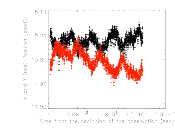
Figure 1: X (black) and Y (red) position of the star centroid in pixels as function of time (binned by 4). These positions are used in the decorrelation function that is used the fit of the transit light curve.

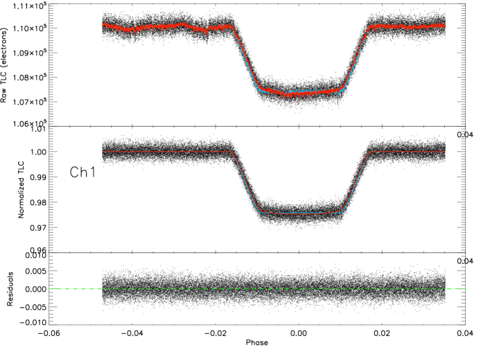
Figure 2: Top panel: raw transit light curve obtained in subarray mode binned by four with its fit overplotted in red. Pixel-phase effect is clearly visible. Middle panel: Normalized transit light curve. Bottom panel: residuals obtained from the fits of the transit light curve.

Due to instrumental effects, our measured out-of-transit flux values are not constant. Telescope pointing jitter results in fluctuations of the stellar centroid position (Fig. 1), which, in combination with intra-pixel sensitivity variations, produces systematic noise in the raw light curves (Fig. 2, upper panel). A description of this effect, known as the pixel-phase effect, is given in the Spitzer/IRAC data handbook (Reach et al. 2006, p. 50; see also Charbonneau et al. 2005). To correct the light curve, we define a baseline function that is the sum of a linear function of time and a quadratic function of the X and Y centroid positions. This function, with five parameters, $K_{i}$, is described in Désert et al. (2009).

We modelled the transit light curve with 4 parameters: the planet-star radius ratio, $R_{p}/R_{\star}$, the orbital semi-major axis to stellar radius ratio (system scale), $a/R_{\star}$, the impact parameter, $b$, and the time of mid transit, $T_{c}$. We used the IDL transit routine OCCULTNL, developed by Mandel & Agol (2002), to model the light curve. Our limb-darkening corrections consist of three non-linear, limb-darkening coefficients, as defined in Sect. 4.3 and presented in Table 1. We also used a linear function of time as the baseline (A_j, $j$=1,2) as presented in Désert et al. (2009).

We used the MPFIT package to perform a Levenberg-Marquardt least-squares fit of the transit model to our cleaned and binned observations. The best-fit model was computed over the whole parameter space ($R_{p}/R_{\star}$, $a/R_{\star}$, $b$, $T_{c}$, $A_{j}$, $K_{i}$). The baseline function described above is combined with the transit light curve function so the fit is constrained by $11$ parameters (4 for the transit model, 2 for the linear baseline, and 5 for the pixel phase effect); this gives $30,039$ degrees of freedom.

3.2 Mean values and errors determination

We used the Prayer Bead method (Moutou et al. 2004, Gillon et al. 2007) to determine the mean value as well as the statistical and systematical errors for the measured parameters.

As shown by Pont et al. (2006), the existence of low-frequency correlated noise (dubbed red noise) between different exposures must be considered to obtain a realistic estimation of the uncertainties. To obtain an estimate of the systematic errors in our observations we followed the method described by Gillon et al. (2006) and derived the covariance from the residuals of the light curve. In the Prayer Bead method, the residuals of the initial fit are shifted systematically and sequentially by one frame, and then added to the transit light curve model before fitting again. The error on each photometric point is the same and is set to the $rms$ of the residuals of the first fit obtained.

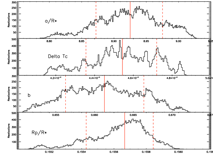
Figure 3: Distributions obtained from the Prayer Bead method for each fitted parameters. Vertical continuous lines correspond to the median of the distribution. Vertical dashed lines correspond to plus or minus 68% of the distribution.

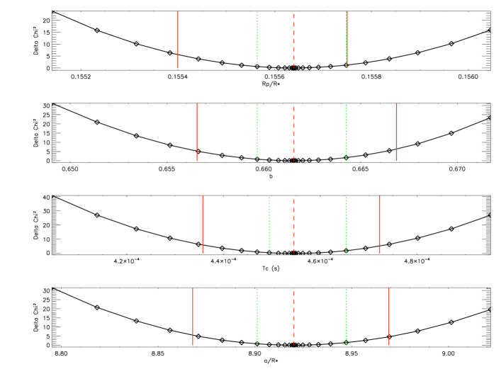
Figure 4: Delta-Khi-square distribution of parameters. Vertical dashed red lines correspond to the values for the minimal Khi-square and vertical continuous red lines correspond to plus or minus $1\sigma$ extracted with the prayer bead method. Vertical dotted green lines correspond to plus or minus $1\sigma$ extracted with the Khi-square method.

Totally, $30050$ shifts and fits of transit light curves were produced to derive a set of parameters and to extract their medians and their corresponding errors. We set our uncertainties equal to the range of values containing $68\%$ of the points in the distribution in a symmetric range about the median for a given parameter (Fig. 3). Error bars estimated using the Prayer Bead method are generally larger than the ones obtained using other methods like ”delta khi square” (Fig. 4) or Markov Chain Monte Carlo (MCMC) because they include the effect of the residual red noise. Therefore these error bars are likely the most conservative.

4 Results and discussion

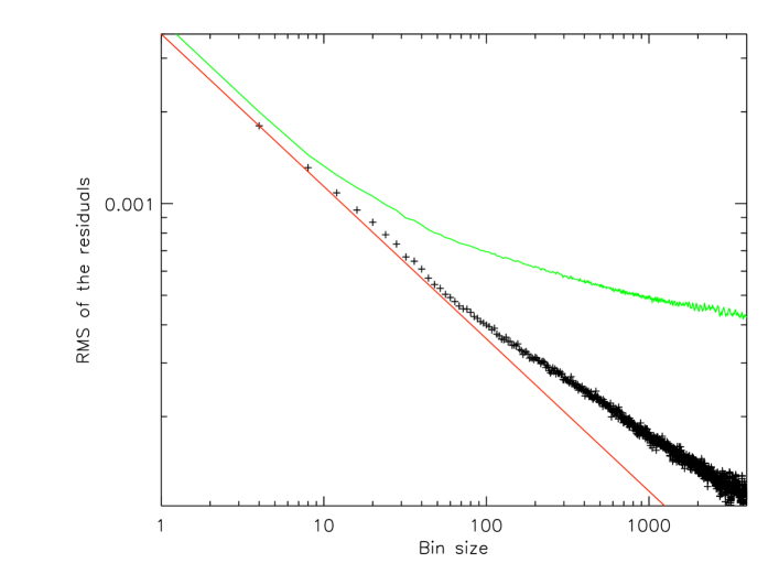
Figure 5: Root-mean-square of binned residuals versus bin size. The solid continuous red line is proportional to $N^{-1/2}$ and is normalized to match the value for bin size $N=4$. Top continuous green curve correspond to bin residuals without pixel-phase decorrelation. Black cross correspond to bin residuals with pixel-phase effect decorrelation. Remaining red-noise become apparent for bin larger than 50 data points (6.25 seconds).

The raw aperture photometry of the transit light curve obtained in subarray mode binned by four is plotted in Figure 2, together with the lightcurve decorrelated from the dependence on instrumental parameters. We derived the system parameters and their error bars in a consistent way using the distribution obtained from the prayer bead method and present the results in Table 2. From our fits, we evaluated the radius ratio $R_{p}/R_{*}$, the impact parameter $b$, the system scale $a/R_{\star}$ and the central time of the transit $T_{c}$ (Table 2). We obtain a mean $\chi^{2}$ of $30024$ for $n=30039$ degrees of freedom. However, we found that the parameters distributions are far from being Gaussian (Fig. 3). This is explained by the presence of a non negligible red-noise left after corrections as revealed by comparing the $rms$ of the unbinned and binned residuals (Fig. 5) following the method described by Gillon et al. (2006). This strenghtens the suggestion that error bars would have been smaller if estimated with methods other than the Prayer Bead.

4.1 Signal-to-noise ratios

The standard deviation of the difference between the best fit model and the observed transit light curve is found to be $1.8\times 10^{-3}$ (rms) on individual data points. This value corresponds to a signal-to-noise of $560:1$ for a frame binned by four; as expected, this is nearly twice the theoretical (photon noise) signal-to-noise ratio for individual frames. We achieve an average of 91% of the theoretical signal-to-noise on individual frames.

We also estimated the red-noise by comparing the $rms$ of residuals with different bin sizes (Fig. 5) and we find that correlated systematics left after decorrelation of the pixel-phase effect have an amplitude of $1.4\times 10^{-4}$ in a bin of a $1000$ points. The amplitude of the white ($\sigma_{w}$) and red ($\sigma_{r}$) noise are obtained by solving the following system of equations:

$$\sigma_{4}^{2} = \frac{\sigma_{w}^{2}}{4}+\sigma_{r}^{2}\;$$ (1)

$$\sigma_{1000}^{2} = \frac{\sigma_{w}^{2}}{1000}+\sigma_{r}^{2}\;\;,$$ (2)

where $\sigma_{4}$ and $\sigma_{1000}$ are the standard deviation taken over a sliding average of four and of one thousand points respectively. We estimated the white noise amplitude, $\sigma_{w}=0.003589$, and the low-frequency red noise amplitude, $\sigma_{r}=0.0001397$.

4.2 Transit timing

The measured central time of the transit can be compared to the expected transit time from a known ephemeris. We measure timing residuals for the transit according to the ephemeris of Knutson et al. (2009) ($P=2.21857578\pm 0.00000080$ days, $Tc=2454399.23990\pm 0.00017$ HJD). We find that the center of our transit is $T_{c}=2454430.310594$ (HJD), which corresponds to an observed minus calculated ($O-C$) transit time of $47s\pm 4(\pm 16)$. The uncertainties are set to the uncertainty in the observed transit time, while the values in parenthesis give the uncertainty in the predicted time. The total uncertainty in the $O-C$ values is the sum of these two values. This corresponds to a time shifted of nearly $3\leavevmode\nobreak\ \sigma$ after its expected value. However, it is difficult to draw conclusion from this result as the determination of mid-transit times are extremely sensitive to fitting the ingress and egress of the eclipse profile. Consequently, correlated noise or a nonuniform stellar brightness distribution could change the ingress/egress shapes of the transit and thus the central time away from what is expected for a uniform stellar disk. A recent study uses seven transits and seven eclipses of this exoplanet to derive a precise set of transit time measurements, with an average accuracy of 3 seconds and reveal a lack of transit-timing variations (Algol et al. 2010).

4.3 Limb darkening

Southworth (2008) shows that the determination of the light curve parameters, especially the radius of the planet, can be sensitive to the applied limb darkening model and its coefficients, yielding a possibility of systematic errors. This is particularly important for transits observed in the visible wavelength, but less important for transits observed in the infrared. Nevertheless, we investigated the importance of stellar limb darkening on the light-curve solutions and parameter uncertainties. We compared our results obtained from fits with various limb darkening laws and different numbers of fit coefficients.

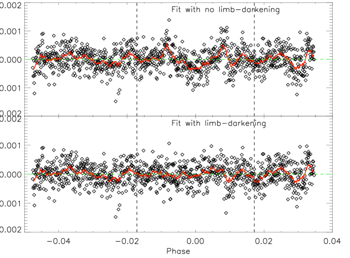
Figure 6: Residuals from fits with or without limb darkening corrections (bottom and top panel respectively). Data (diamonds) are binned by 120 ( 15 seconds) and a smooth of these binned residuals is overplot in red. Vertical dashed lines mark the beginning and the end of the transit (first and last contact). The fit is better with limb darkening. No signature remains in the residuals.

We first note that the fit is clearly improved when including limb darkening (Fig. 6). We found that accounting for the effects of limb-darkening at 3.6 $\mu$m decreased the resulting best-fit transit depth by $(\Delta R_{p}/R_{\star})_{3.6\leavevmode\nobreak\ \mu m}=0.0005$ which corresponds to $5\leavevmode\nobreak\ \sigma$ in the present result. We used a non linear limb darkening law with three fixed limb darkening coefficients (Table 1) which is slightly different from the one used in Désert et al. (2009). In the present work, we set $c_{1}$ to zero and calculate new sets of coefficients c₂, c₃ and c₄, resulting in a three-parameter non-linear limb darkening law,

$$\frac{I(\mu)}{I(1)}=1-c_{2}(1-\mu)-c_{3}(1-\mu^{3/2})-c_{4}(1-\mu^{2})$$ (3)

The $c_{1}(1-\mu^{1/2})$ term was removed because it reflects the intensity distribution at small $\mu$ values and is not needed when the intensity at the limb is desired to vary linearly at small $\mu$ values (for further details see Sing et al. 2009 and Sing et al. 2010.) Compared to the quadratic law, the added $\mu^{3/2}$ term provides the flexibility needed to more accurately reproduce the stellar model atmospheric intensity distribution at near-infrared and infrared wavelengths. The limb darkening coefficients for the three-parameter non-linear law were computed using a Kurucz ATLAS stellar model with T_eff=5000 K, log g=4.5, and [Fe/H]=0.0 in conjunction with the transmission through the IRAC filters and fitted the calculated intensities between $\mu$=0.05 and $\mu$=1 (Table 1). This limb darkening law is slightly different from the one used in the previous analysis (Désert et al. 2009) particularly at the limb ($\mu<0.05$). Nevertheless, the signal-to-noise ratio of our data is not high enough to distinguish the changes between the two sets of limb darkening coefficients since the difference in the normalized transit light curves is less than $10^{-6}$.

The photometric precision of our transit light curve allowed us to perform fits using a non-linear limb-darkening model with the linear coefficient ($c_{2}$) as a free parameter. We find c${}_{2}=1.12994\pm 0.0243$ in agreement with the value quoted in Table 1. As a test, we also fitted the transit light curve using a linear limb darkening law with one single coefficient c₁ as free parameter. We derived c${}_{1}=0.27821\pm 0.0291$ and find that $R_{p}/R_{\star}$ is $2.5\sigma$ above the solution obtained with a the non-linear limb darkening law, but with a less good $\chi^{2}$, showing that this solution can be excluded and the non-linear law is preferred.

4.4 Comparison with previous observations

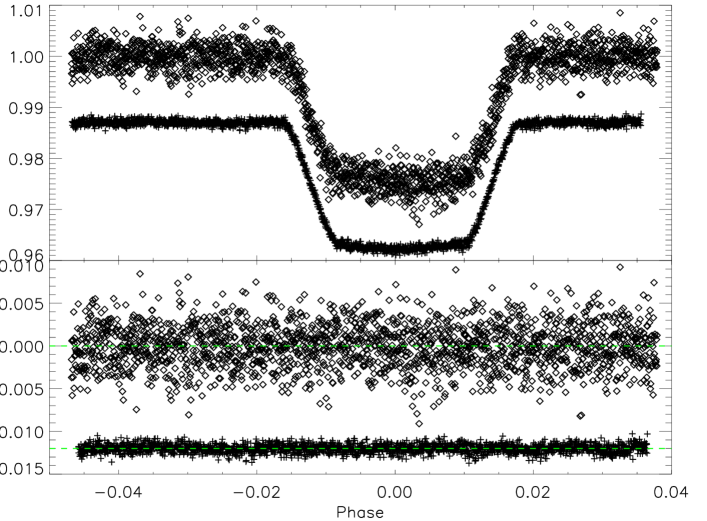
Figure 7: Top panel: normalized transit light curves obtained in Stellar mode (diamonds) and in Subarray mode (crosses). The Subarray mode transit light curve is shifted vertically for display purpose. The Subarray mode transit light curve is binned by 64 to obtained the same number of data points ($\sim 1900$ points) as the Stellar mode transit light curve. Bottom panel: residuals obtained from the fits of the transit light curve. Residuals from the binned Subarray mode transit light curve are shifted vertically (for display) and are 4 times smaller.

We compare the parameters derived here with the results obtained from visit 1 and 2 observations (Désert et al. 2009). Results from fits to the transit light curve obtained in visit 1 observations obtained at 3.6 $\mu$m are summarized in Table 2. We measured a dispersion of $2.1\times 10^{-3}$ (rms) on the individual $\sim 1900$ data points with an exposure time of 0.4 s. This corresponds to a ${\rm S/N}$ of 400:1 per image. To compare with our present data set, we binned the visit 3 transit light curve by $64$ and obtained $\sim 1900$ points with a $rms=4.9\times 10^{-4}$. The two transit light curves, obtained for visit 1 and 3 at 3.6 $\mu$m, are overplotted with 1900 points each in Fig. 7. The $S/N$ by subarray frame is four times higher than by stellar mode exposure, in agreement with expected photon noise for a total exposure time sixteen times longer.

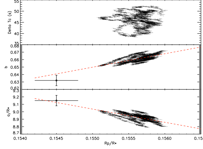
Figure 8: Joint distributions of parameters obtain from the Prayer Bead method using the subarray mode observations. The x-axis corresponds to radius ratios for all the panels. The top panel is the fit of the central time, the middle and bottom panel corresponds to the impact parameter and the scale of the system respectively. The diamonds with error bars correspond to the results obtain from visit 1 observations (Désert et al. 2009). The dashed red lines correspond to linear fits of the points from visit 3, and reveal the correlations between $R_{p}/R_{\star}$, $b$ and $a/R_{\star}$.

We are particularly interested in the comparison of the ratios of the radius of the planet over the radius of the star at 3.6 $\mu$m in the two observation sets. The radius ratio found in visit 3 stands $4\sigma$ above the value derived from visit 1 at 3.6 $\mu$m (Table 2). The impact parameters $b$ and system scales $a/R_{\star}$ measured in the transit light curves provide informations for interpreting these results. We found that the $b$ and $a/R_{\star}$ values derived from visit 1 observations at 3.6 $\mu$m, are respectively $3\sigma$ below and above the values obtained here at the same wavelength with visit 3 observations (Fig. 8 and 9). The same results are obtained for visit 1 observations at 5.8 $\mu$m (both observations at 3.6 $\mu$m and 5.8 $\mu$m were accumulated simultaneously during visit 1). As already noticed in Désert et al. (2009), the $b$ and $a/R_{\star}$ measured with visit 1 and 2 stellar mode observations are consistent between channels observed simultaneously, but disagree between channels observed at two different epochs. This suggests that unrecognized systematics remains between the observations obtained at the two epochs. This systematic effect could be either instrumental or astrophysical. Below, we estimate the impact of those systematics on the radius determination, and possible astrophysical origins of these discrepancies.

The value of the impact parameter $b$ has a direct effect on the derived planetary radius. This can be seen theoretically from the analytic approximation (Carter et al. 2008):

$$b^{2}=1-\frac{T}{\tau}\times\frac{R_{p}}{R_{\star}}$$ (4)

where $\tau$ is the ingress or egress duration($\tau=t_{\rm II}-t_{\rm I}$), $t_{\rm I}$ and $t_{\rm II}$ are the time of first and second contact, and $T$ is the total transit duration. Consequently, underestimating the $b$ from $0.66$ to $0.63$, without changing the timing of ingress and egress would lead to overestimate $R_{p}/R_{\star}$ by $0.001$, which corresponds to $10\leavevmode\nobreak\ \sigma$ in the result from visit 3.

We estimated the influence of systematic errors on the estimate of $b$ on the determination of the radius.

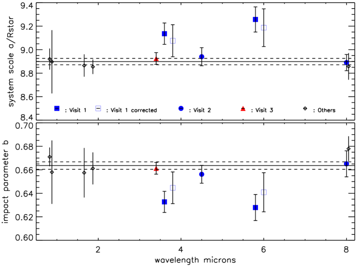
Figure 9: Orbital parameters derived from several studies. Top panel: impact parameter $b$, Bottom panel: system scale $a/R_{\star}$. Diamonds are values from several other studies: data are from Pont et al. (2007) in the visible, from Sing et al (2009) in the near infrared and from Knutson et al. (2007) at 8.0$\mu$m also measured by Carter & Winn (2010). Blue squares are from our visit 1 and 2 observations in the four IRAC channels (Désert et al. 2009). The red square are from visit 3 observations (this work). Continuous and dashed straight black lines indicate the average and error values obtained from data excluding outliers. These values are considered as best estimates for $b$ and $a/R_{\star}$. Parameters derived from visit 1 at 3.6 and 5.8 $\mu$m respectively, are significantly different from the best estimates. The empty squares corresponds to the derived parameters using to the visit 1 observation and transit light curve model which take into account occulted spots during ingress or egress.

We fixed the $b$ value of visit 1 to the one obtained at higher $S/N$ in visit 3 ($b=0.661$) and fitted visit 1 transit light curves at 3.6 $\mu$m and 5.8 $\mu$m. In that case, for visit 1, we obtained $(R_{p}/R_{\star})_{3.6\,\mu\mathrm{m}}=0.15532$; these values are in agreement with the results obtained in visit 3 (Fig. 9).

In conclusion, we find consistent values for $R_{p}/R_{\star}$ and $a/R_{\star}$ in all data sets if the impact parameters $b$ is set to the same value. Our final value is in agreement with the values $b=0.671\pm 0.008$ and $a/R_{\star}=8.92\pm 0.09$ derived by Pont et al. (2008) with HST/ACS, with the values obtained by Sing et al. (2009) with HST/NICMOS, and with $a/R_{\star}=8.924\pm 0.022$ from Carter & Winn (2010) using several Spitzer/IRAC transit light curves at 8 $\mu$m. This suggests that $b$ and $a/R_{\star}$ derived from visit 1 are affected by unknown systematics which could be either instrumental or astrophysical such as starspots (see next section 4.5).

4.5 Impact of starspots on the derived parameters

HD 189733 is an active K star, which has been observed to vary photometrically by $\pm 1.5$% at visible wavelengths (Henry & Winn  2008; Croll et al. 2007; Miller-Ricci et al. 2008). Those variations are caused by rotational modulations in the visibility of star spots on a rotation period of $11.953\pm 0.009$ days (Hébrard & Lecavelier des Etangs 2006; Henry & Winn 2008).

In this section, we consider the possibility that transit light curves can be modified by the presence of spots on the surface of the star, introducing systematic errors on the parameters estimates. In particular, we investigate the possible contribution of stellar spots and brightness inhomogeneities to explain the discrepancy between the planet radii at 3.6 $\mu$m measured in visits 1 and 3 data (Sect.4.5.2). We also investigate the effect of spots to explain the bias in the orbital parameters estimated using visit 1 data (Sect. 4.5.3).

4.5.1 Ground based photometric follow-up

We use ground based photometric follow-up to estimate and to correct for the stellar activity at the epochs of our 3 visits observations.

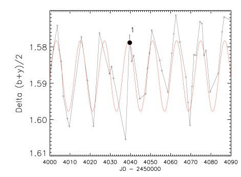
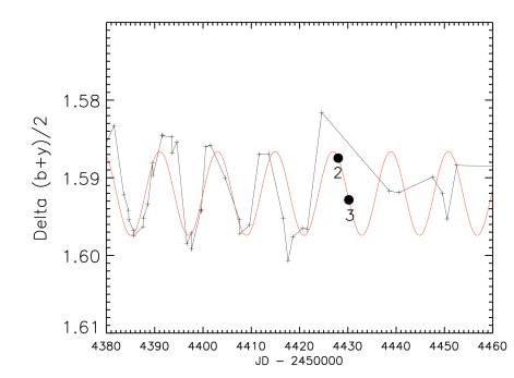
Figure 10: a. (top). Relative flux variation for HD 189733 observed with ground-based follow-up encompassing the time of our IRAC observations (connected crosses). Black circular spot indicates the time of our Spitzer Stellar mode observations at 3.6 and 5.8 $\mu$m (Visit 1). Variations are caused by rotational modulation in the visibility of star spots with a rotation period of 11.953 days (Henry & Winn 2008). The continuous curve overplotted in red corresponds to a sinusoid with a period of 11.95 days. b. (bottom). The same as above for the stellar mode observations at 4.5 and 8.0 $\mu$m (Visit 2) and Subarray mode observations at 3.6 $\mu$m (Visit 3).

The star has been followed-up in V-band over several years using the Tennessee State University $0.8\leavevmode\nobreak\ m$ automated photometric telescopes (APT) at Fairborn Observatory (Henry et al. 2008). These data show that the stellar flux variation reach a peak to peak maximum of $3\%$ in the visible (Fig. 10).

The observed variations in the visible have to be translated to corresponding variation in the infrared. Let’s define $f_{\lambda}$, the relative variation in flux due to stellar activity:

$$f_{\lambda}\equiv\frac{F_{\star}(\lambda)-F_{quiet}(\lambda)}{F_{quiet}(\lambda)},$$ (5)

where $F_{\star}$ is the measured flux and $F_{quiet}$ is the reference stellar flux (e.g., without stellar activity). $f_{\lambda}$ is negative when the star is fainter and positive when it is brighter than the reference brightness.

Previous HST ACS observations of HD 189733 have established that its stellar spots have an effective temperature approximately 1000 K cooler than that of the stellar photosphere (Pont et al. 2008) with spot size $\sim 2.8\%$ of the stellar disk area. Following Knutson et al. (2009), we considered that the amplitude of the stellar flux variations scales approximately as the ratio of the flux of blackbodies at 5000 and 4000 K. Thus, we used the normalized difference of Planck functions to estimate the maximum variation of flux at 3.6$\mu$m $f_{(3.6\mu m)}$. The $3\%$ maximum variation in the V-band due to the presence of spots on the stellar surface, scales to $f_{(3.6\mu m)}\sim 0.8\%$ in the infrared.

The ground-based photometry suggests that visit 1 happened during the maximum brightness of the star (Fig. 10). Unfortunately, no ground based observations were acquired during visit 2 and 3. Thus, we have no direct measurement of the stellar activity at those precise epochs. Nevertheless, the activity period $P=11.953\pm 0.009$ (Henry & Winn 2008) can be used to interpolate the star brightness at the epochs of visit 2 and 3. We found that the star should be close to its maximal brightness during visit 2, and $\sim 2\%$ below the maximal brightness during visit 3, corresponding to $f_{(3.6\mu m)}\sim-0.5\%$ at this epoch.

4.5.2 Stellar spots outside the zone occulted by the planet

Spots and bright faculae cause variations in the star brightness ($F_{\star}$). Nonetheless, if the surface brightness of the zone occulted by the planet is not modified, the absolute depth of the transit light curve ($\Delta F_{\star}$) remains the same. Therefore, at epoch of low stellar brightness like during visit 3, the relative transit depth ($\Delta F_{\star}/F_{\star}$) can be significantly overestimated, leading to an overestimate of the planet to star radius ratio.

As seen in Corot-2b (Czesla et al. 2009), the transit depth constraining the planet radius ratio is correlated with the star brightness. We can empirically define $\alpha$ by:

$$\frac{\left(\frac{R_{p}}{R_{\star}}\right)_{Measured}^{2}-\left(\frac{R_{p}}{R_{\star}}\right)_{True}^{2}}{\left(\frac{R_{p}}{R_{\star}}\right)_{True}^{2}}=\alpha f_{\lambda},$$ (6)

where $(R_{p}/R_{\star})_{True}$ is the true radius ratio which could be obtained from the transit light curve when the star presents no spots and is at the reference brightness. The relative error on the measured radius ratio is therefore given by :

$$\frac{\Delta(R_{p}/R_{\star})}{\left(R_{p}/R_{\star}\right)_{True}}\approx\frac{\alpha f_{\lambda}}{2},$$ (7)

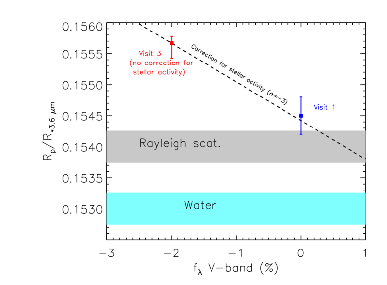
Figure 12: Measured values of $R_{p}/R_{\star}$ ratios at 3.6 $\mu$m as fonction of the relative decrease of stellar flux due to spots (in V-band). The blue and red squares are the $R_{p}/R_{\star}$ derived from visit 1 and 3 observations respectively. The dotted line corresponds to the theoretical correction of the relative difference between the measured radius ratio and the expected value as fonction of the relative decrease of stellar flux in the V-band $f_{\lambda}$. Using ground based photometric follow-up (Fig. 10), we set $f_{(3.6\leavevmode\nobreak\ \mu m)}$ to zero for visit 1 (see text 4.5.1). The $R_{p}/R_{\star}$ we derive from visit 3 observations (no correction) is above the one obtained in visit 1 ($4\leavevmode\nobreak\ \sigma$). To compare both visits, the $R_{p}/R_{\star}$ derived from visit 3 has to be corrected for spots (Sect. 4.5.3). Simultaneous observation in V-band shows that $f_{V-band}=-2\%$ during visit 3 (Fig. 10). $(R_{p}/R_{\star})_{Corrected}$ for visit 3 is in agreement with $R_{p}/R_{\star}$ derived in visit 1 for a slope $\alpha=-3$.

In Corot-2b data (Czesla et al. 2009), we found $\alpha\sim 1.7$. With the hypothesis that the stellar surface brightness outside the spot areas is not modified by the stellar activity, we obtained $\alpha=-1$. With the photometric variations obtained from ground based observation at epochs close to the Spitzer observations, we found $f_{3.6\mu m}=-0.5\%$ in visit 3 compared to visit 1. Therefore, the radius ratio $R_{p}/R_{\star}$ derived from visit 3 which is $\sim 0.75\pm 0.18\%$ above the radius derived from visit 1 (Table 2) can be explained using equation 7 if $\alpha\sim-3\pm 1$ (Fig. 12).

In short, the discrepancy between the visit 1 and 3 radius ratios at 3.6 $\mu$m can be explained by the effect of stellar activity and the presence of spots during the visit 3.

4.5.3 Occulted starspots

The planet occulting dark or bright areas on the surface of the star during transit produces a rise or decrease in the flux. Because the ingress and egress parts of the transit light curve strongly constrain the orbital parameters of the planet, dark or bright areas occulted by the planet during the ingress or egress change the apparent time of the transit contacts, introducing systematic errors in the derived $b$ and $a/R_{\star}$ parameters (Eq. 4). Consequently, the low $b$ value obtained in channel 1 and 3 using visit 1 data could be caused by the presence of cold spots or bright faculae occulted by the planet.

To estimate the influence of occulted star cold or bright regions during the ingress and egress on the determination of our parameters, we fitted the visit 1 and 2 observations with a transit light curve model including occulted star spots (cold or hot) during ingress and egress. These fits have a goodness of fit equivalent to the fits using the model without spots. For visit 2, the model with occulted spots give similar results as Désert et al. (2009). Most importantly, for visit 1, the model fits well the data with a bright spot occulted during the ingress part of the light curve. The best fit is found assuming a spot size similar to the size of the planet and a spot surface brightness $8\%$ brighter than the star. Compared to the results given in Désert et al. (2009), this new model applied to visit 1 data at 3.6 $\mu$m gives a larger $b$ by 0.013 ($2\leavevmode\nobreak\ \sigma$), a smaller $a/R_{*}$ by 0.06 ($1\leavevmode\nobreak\ \sigma$), and error bars larger by a factor of about $1.5$. Interestingly, the $R_{p}/R_{*}$ found with this new model changes by less than $0.3\leavevmode\nobreak\ \sigma$. Similar conclusion are obtained with data at 5.8 $\mu$m (Fig. 9).

As a conclusion, the surprising results for $b$ and $a/R_{*}$ found by Désert et al. (2009) in visit 1 data can simply be explained by astrophysical systematics in the transit light curve due to stellar activity. However, the difference in the measured values for the radius ratios $R_{p}/R_{\star}$ between Visit 1 and 3 cannot be explained by such dark and bright areas occulted during ingress or egress. It must be caused by the fluctuation of the whole stellar disk brightness (see Sect. 4.5.2).

4.6 Opacities in the IRAC bandpasses

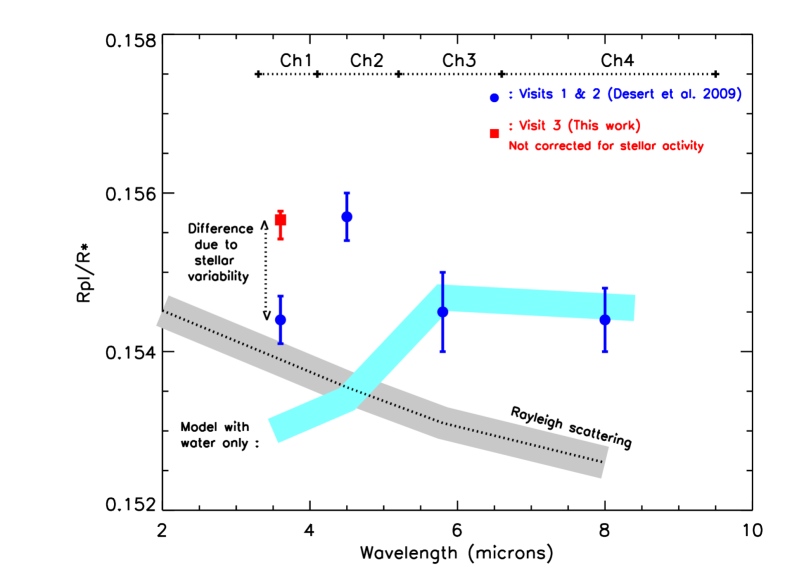
Figure 11: Census of the measured values of $R_{p}/R_{\star}$ ratios in the four Spitzer/IRAC channels for HD 189733b obtained using three transit observations during visit 1 and 2 (blue circles; D sert et al. 2009), and visit 3 (red square; this work) with their $1\leavevmode\nobreak\ \sigma$ error bars. The data point obtained for visit 3 has to be corrected from stellar spots (see text 4.5.3). The IRAC bandpasses for each channel are shown at the top with dotted line. The theoretical planet-to-star radius ratios with absorption by only water molecules or by only Rayleigh scattering are plotted in light blue and grey respectively.

The $R_{p}/R_{\star}$ measured at 3.6 $\mu$m from visit 1 is $4\leavevmode\nobreak\ \sigma$ above the value measured in visit 3. This difference can be reconciled by correcting for the $2\leavevmode\nobreak\ \%$ stellar variability monitored with the ground-based observations between the two visits. However, at least two colors measured simultaneously are required to ensure that the measured variations of the wavelength dependant radius of the planet are caused by the presence of atmospheric chemical absorbers. In this framework, the $R_{p}/R_{\star}$ measured at 3.6 $\mu$m from visit 1 is $4\leavevmode\nobreak\ \sigma$ above the opacity due to water if we consider that the radius simultaneously measured at 5.8 $\mu$m is due to water opacity. Therefore, other species beyond H₂O must be present in the atmosphere of the planet and absorb at 3.6 $\mu$m. One possible physical explanation for the large radius at 3.6 $\mu$m could be due to Rayleigh scattering (Lecavelier des Etangs et al. 2008b). Effectively, the radius mesured at this wavelength is in agreement at one sigma level with its expected value if we consider Rayleigh scattering opacity (Fig. 11). We note that the possible presence of a strong methane (CH₄) band at 3.3 $\mu$m could also contribute to the opacity in this bandpass (Sharp & Burrows 2007). The radius we derived at 4.5 $\mu$m could be interpreted as due to CO molecules which exhibit a large opacities in this bandpass (Désert et al. 2009). The radii we derived at 5.8 $\mu$m and 8.0 $\mu$m are at more than $3\leavevmode\nobreak\ \sigma$ above the absorption due to Rayleigh scattering, and could be interpreted by the presence of water molecules which opacity overcomes Rayleigh scattering at those wavelengths (Fig. 11). These two bandpasses exhibit approximatly the same radius value, consistent with a model which includes water.

Therefore water vapour could be present in the atmosphere of this hot-Jupiter ; but it cannot be evidenced simply comparing planetary radii measured at 3.6 and 5.8 $\mu$m, because the radius measured at 3.6 $\mu$m is affected by some other species absorption.

5 Conclusion

We obtained a new high-$S/N$ photometric transit light curve at 3.6 $\mu$m using the IRAC/Spitzer subarray mode observations. This observing mode offers a higher photometric cadence, therefore a better signal-to-noise ratio than the previous measurements (stellar mode) obtained at this wavelength. We derive a value of $R_{p}/R_{\star}=0.15566\pm 0.00011$ at 3.6 $\mu$m which is $4\sigma$ above the value derived from previous observations in the same bandpass (Désert et al. 2009). This difference is explained by the stellar variability between the two observational epochs. Simultaneous ground based observation allowed us to correct for these variations. A photometric variation of $\sim 2\%$ in V-band was monitored between the two measurements and provide a correction of $-0.75\%$ for the new 3.6 $\mu$m measurement. Noteworthy, the first observation was obtained during the maximum brightness of the star, which led to the minimal possible value of the measured $R_{p}/R_{\star}=0.1545\pm 0.0003$ at 3.6 $\mu$m for this planet (Désert et al. 2009). This final planet-to-star radius ratio at 3.6 $\mu$m is above the expected value if only water molecules were contributing to the absorption at both 3.6 and 5.8$\mu$m.

We showed the importance of long term ground based monitoring program in order to take into account the stellar activity and to compare results obtained from observations carried out at different epochs. Any estimate of the planet to star radius ratio should be associated with a corresponding stellar activity level.

Visit	C1	C2	C3	C4
1 (Désert et al. 2009)	0.6023	-0.5110	0.4655	-0.1752
3 (This work)	0.0000	1.13694	-1.3808	0.55045

Table 1: Limb darkening coefficients used for IRAC/channel 1 bandpass centered at 3.6 $\mu$m. The coefficients are the ones used for visit 3 (this study) and used in our previous analysis (visit 1; see Désert et al. 2009). The two sets of coefficients only differ at the limb (see Sect. 4.3)

Parameter at $3.6\leavevmode\nobreak\ \mu m$	Median (visit 3)	$1\sigma(68\%)$	$2\sigma(95\%)$	visit 1 (Désert et al. 2009)
$R_{p}/R_{\star}$	$0.15566$	${}^{+0.00011}_{-0.00024}$	${}^{+0.00022}_{-0.00043}$	$0.1545\pm 0.0003$
$b$	$0.6613$	${}^{+0.0053}_{-0.0050}$	${}^{+0.0078}_{-0.0079}$	$0.632\pm 0.007$
$a/R_{\star}$	$8.925$	${}^{+0.049}_{-0.052}$	${}^{+0.079}_{-0.096}$	$9.15\pm 0.07$
$T_{c}(s)$	$47$	${}^{+3.4}_{-3.6}$	${}^{+5.0}_{-6.4}$	$19\pm 12$

Table 2: Fitted parameters of the transit light curves at 3.6 $\mu$m for Visit 1 and 3. Quoted errors corresponds to 68% and 95% of the realizations (Visit 3).

- (1) Agol, E., Cowan, N. B., Bushong, J., Knutson, H., Charbonneau, D., et al. 2008, arXiv:0807.2434
- (2) Agol, E., Cowan, N. B., Knutson, H. A., Deming, D., Steffen, J. H., Henry, G. W., & Charbonneau, D. 2010, arXiv:1007.4378
- (3) Bakos, G. Á., Knutson, H., Pont, F., Moutou, C., Charbonneau, D., et al. 2006b, ApJ, 650, 1160
- (4) Bakos, G. Á., Pál, A., Latham, D. W., Noyes, R. W., & Stefanik, R. P. 2006a, ApJ, 641, L57
- (5) Ballester, G. E., Sing, D. K., & Herbert, F. 2007, Nature, 445, 511
- (6) Beaulieu, J. P., Carey, S., Ribas, I., & Tinetti, G. 2008, ApJ, 677, 1343
- (7) Bouchy, F., et al. 2005, A&A, 444, L15
- Burrows et al. (2008) Burrows, A., Budaj, J., & Hubeny, I. 2008, ApJ, 678, 1436
- (9) Burrows, A., Hubbard, W. B., Lunine, J. I., & Liebert, J. 2001, Reviews of Modern Physics, 73, 719
- Carter et al. (2008) Carter, J. A., Yee, J. C., Eastman, J., Gaudi, B. S., & Winn, J. N. 2008, ApJ, 689, 499
- Carter & Winn (2010) Carter, J. A., & Winn, J. N. 2010, ApJ, 709, 1219
- Charbonneau et al. (2008) Charbonneau, D., Knutson, H. A., Barman, T., Allen, L. E., Mayor, M., Megeath, S. T., Queloz, D., & Udry, S. 2008, ApJ, 686, 1341
- (13) Charbonneau, D., Allen, L. E., Megeath, S. T., et al. 2005, ApJ, 626, 523
- (14) Charbonneau, D., Brown, T. M., Noyes, R. W., & Gilliland, R. L. 2002, ApJ, 568, 377
- Croll et al. (2007) Croll, B., et al. 2007, ApJ, 671, 2129
- Czesla et al. (2009) Czesla, S., Huber, K. F., Wolter, U., Schröter, S., & Schmitt, J. H. M. M. 2009, A&A, 505, 1277
- (17) Deming, D., Harrington, J., Laughlin, G., et al. 2007, ApJ, 667, L199
- (18) Deming, D., Harrington, J., Seager, S., & Richardson, L. J. 2006, ApJ, 644, 560
- (19) Deming, D., Seager, S., Richardson, L. J., & Harrington, J. 2005, Nature, 434, 740
- Demory et al. (2007) Demory, B.-O., Gillon, M., Barman, T. et al. 2007, A&A, 475, 1125
- (21) Désert, J.-M., Vidal-Madjar, A., Lecavelier Des Etangs, A., Sing, D., Ehrenreich, D., et al. 2008, A&A, 492, 585
- (22) Désert, J. -M., Lecavelier des Etangs, A., et al. 2009, arXiv:0903.3405 (in press)
- (23) Ehrenreich, D., Hébrard, G., Lecavelier des Etangs, A., et al. 2007, ApJ, 668, L179
- (24) Fazio, G. G., et al. 2004, ApJS, 154, 10
- Fortney et al. (2008) Fortney, J. J., Lodders, K., Marley, M. S., & Freedman, R. S. 2008, ApJ, 678, 1419
- (26) Fortney, J. J., & Marley, M. S. 2007, ApJ, 666, L45
- (27) Gillon, M., Demory, B.-O., Barman, T., et al. 2007, A&A, 471, L51
- (28) Gillon, M., Pont, F., Moutou, C., Bouchy, F., Courbin, F., et al. 2006, A&A, 459, 249
- (29) Grillmair, C. J., Burrows, A., Charbonneau, D., Armus, L., Stauffer, J., et al. 2008, Nature, 456, 767
- Grillmair et al. (2007) Grillmair, C. J., Charbonneau, D., Burrows, A., Armus, L., Stauffer, J., Meadows, V., Van Cleve, J., & Levine, D. 2007, ApJ, 658, L115
- Hebrard et al. (2010) Hebrard, G., et al. 2010, arXiv:1004.0790
- (32) Hébrard, G., & Lecavelier des Etangs, A. 2006, A&A, 445, 341
- Henry & Winn (2008) Henry, G. W., & Winn, J. N. 2008, AJ, 135, 68
- (34) Hubbard, W. B., Fortney, J. J., Lunine, J. I., et al. 2001, ApJ, 560, 413
- (35) Knutson, H. A., Charbonneau, D., Noyes, R. W., Brown, T. M., & Gilliland, R. L. 2007a, ApJ, 655, 564
- (36) Knutson, H. A., et al. 2007b, Nature, 447, 183
- (37) Kurucz R. 2006, Stellar Model and Associated Spectra (http://kurucz.harvard.edu/grids.html)
- (38) Lecavelier des Etangs, A., Ehrenreich, D., Vidal-Madjar, A., et al. 2010, A&A, 514, A72
- (39) Lecavelier des Etangs, A., Pont, F., Vidal-Madjar, A., & Sing, D. 2008a, A&A, 481, L83
- (40) Lecavelier des Etangs, A., Vidal-Madjar, A., Désert, J.-M., & Sing, D. 2008b, A&A, 485, 865
- (41) Mandel, K., & Agol, E. 2002, ApJ, 580, L171
- Miller-Ricci et al. (2008) Miller-Ricci, E., et al. 2008, ApJ, 682, 593
- (43) Moutou, C., Pont, F., Bouchy, F., & Mayor, M. 2004, A&A, 424, L31
- Nutzman et al. (2009) Nutzman, P., Charbonneau, D., Winn, J. N., Knutson, H. A., Fortney, J. J., Holman, M. J., & Agol, E. 2009, ApJ, 692, 229
- (45) Pont, F., Zucker, S., & Queloz, D. 2006, MNRAS, 373, 231
- (46) Pont, F., Gilliland, R. L., Moutou, C., Charbonneau, D., Bouchy, F., et al. 2007, A&A, 476, 1347
- (47) Pont, F., Knutson, H., Gilliland, R. L., Moutou, C., & Charbonneau, D. 2008, MNRAS, 385, 109
- (48) Reach, W. T., et al. 2006, IRAC Data Handbook v3.0
- (49) Redfield, S., Endl, M., Cochran, W. D., & Koesterke, L. 2008, ApJ, 673, L87
- (50) S. Czesla, K. F. Huber, U. Wolter, S. Schr ter, J. H. M. M. Schmitt, submitted
- (51) Seager, S.,& Sasselov, D. D. 2000, ApJ, 537, 916
- (52) Sing, D. K., Vidal-Madjar, A., Désert, J. -M., Lecavelier des Etangs, A., & Ballester, G. 2008a, ApJ, 686, 658
- (53) Sing, D. K., Vidal-Madjar, A., Lecavelier des Etangs, A., et al. 2008b, ApJ, 686, 667
- Sing et al. (2009) Sing, D. K., Désert, J.-M., Lecavelier Des Etangs, A., Ballester, G. E., Vidal-Madjar, A., Parmentier, V., Hebrard, G., & Henry, G. W. 2009, A&A, 505, 891
- Sing (2010) Sing, D. K. 2010, A&A, 510, A21
- (56) Sharp, C. M., & Burrows, A. 2007, ApJS, 168, 140
- Southworth (2008) Southworth, J. 2008, MNRAS, 386, 1644
- (58) Swain, M. R., Vasisht, G., & Tinetti, G. 2008, Nature, 452, 329
- (59) Swain, M. R., Vasisht, G., Tinetti, G., Bouwman, J., Chen, P., et al. 2009, ApJ, 690, L114
- (60) Tinetti, G., et al. 2007b, Nature, 448, 169
- (61) Vidal-Madjar, A., Lecavelier des Etangs, A., Désert, J.-M., et al. 2008, ApJ, 676, L57
- (62) Vidal-Madjar, A., et al. 2004, ApJ, 604, L69
- (63) Vidal-Madjar, A., Lecavelier des Etangs, A., Désert, J.-M., Ballester, G. E., Ferlet, R., Hébrard, G., & Mayor, M. 2003, Nature, 422, 143
- (64) Werner, M. W. et al., 2004, ApJS, 154, 1
- (65) Winn, J. N., et al. 2007, AJ, 133, 1828