Milky Way Disk-Halo Transition in H I: Properties of the Cloud Population

Abstract

Using 21 cm H I observations from the Parkes Radio Telescope’s Galactic All-Sky Survey, we measure 255 H I clouds in the lower Galactic halo that are located near the tangent points at $16.9\arcdeg\leq l\leq 35.3\arcdeg$ and $|b|\lesssim 20\arcdeg$. The clouds have a median mass of 700 M_⊙ and a median distance from the Galactic plane of 660 pc. This first Galactic quadrant (QI) region is symmetric to a region of the fourth quadrant (QIV) studied previously using the same data set and measurement criteria. The properties of the individual clouds in the two quadrants are quite similar suggesting that they belong to the same population, and both populations have a line of sight cloud-cloud velocity dispersion of $\sigma_{cc}\approx 16$ km s^-1. However, there are three times as many disk-halo clouds at the QI tangent points and their scale height, at $h=800$ pc, is twice as large as in QIV. Thus the observed line of sight random cloud motions are not connected to the cloud scale height or its variation around the Galaxy. The surface density of clouds is nearly constant over the QI tangent point region but is peaked near $R\sim 4$ kpc in QIV. We ascribe all of these differences to the coincidental location of the QI region at the tip of the Milky Way’s bar, where it merges with a major spiral arm. The QIV tangent point region, in contrast, covers only a segment of a minor spiral arm. The disk-halo H I cloud population is thus likely tied to and driven by large-scale star formation processes, possibly through the mechanism of supershells and feedback.

1. Introduction

The atomic hydrogen (H I) in the Milky Way has long been known to lie in a thin layer with a FWHM of a few hundred pc in the inner Galaxy (Schmidt, 1957). The layer, however, consists of multiple components, each with a different scale height, and the densest and coolest gas is more confined to the Galactic plane than the warmer, more diffuse gas (Baker & Burton, 1975; Lockman, 1984; Savage & Massa, 1987; Dickey & Lockman, 1990; Savage & Wakker, 2009). The connection between scale height and physical temperature seems natural but is misleading, for temperature alone is not sufficient to support any of the H I components to their observed height — additional support is needed, most likely from turbulence. In the vicinity of the Sun it is plausible that the observed turbulence is sufficient to support the H I layer (Lockman & Gehman, 1991; Koyama & Ostriker, 2009), but in the inner Galaxy, at a Galactocentric radius $R\approx 4$ kpc, one H I component has an exponential scale height of 400 pc (Dickey & Lockman, 1990), and would require a turbulent velocity dispersion $\sigma_{z}>70$ km s^-1 to achieve its vertical extent (Kalberla & Kerp, 2009). Evidence for the existence of a medium with these properties is contradictory (Kalberla et al., 1998; Howk et al., 2003). The H I component with the largest scale height may be involved in circulation of gas between the disk and halo, and probably contains the majority of the kinetic energy of the neutral ISM (Kulkarni & Fich, 1985; Lockman & Gehman, 1991).

The discovery that the transition region between the Galactic disk and halo in the inner Galaxy contains many discrete H I clouds that have a spectrum of size and mass, and that follow normal Galactic rotation to several kpc from the plane (Lockman, 2002), changed the picture considerably. A significant fraction of the H I far from the Galactic plane may be contained in these clouds, which are clearly part of a disk population unrelated to high-velocity clouds. They are much denser than their surroundings, but do not have the density needed for gravitational stability. Because the H I clouds are seen in a continuous distribution from the Galactic disk up to several kpc into the halo (Stil et al., 2006; Lockman, 2002), we will refer to them as disk-halo clouds. Clouds with similar properties have been detected in the outer Galaxy (Stanimirović et al., 2006; Dedes & Kalberla, 2010). Their origin, lifetime, evolution, and connection with other interstellar components is unknown. They might result from a galactic fountain (Shapiro & Field, 1976; Bregman, 1980; Houck & Bregman, 1990; Spitoni et al., 2008), H I shells and supershells (McClure-Griffiths et al., 2006), or interstellar turbulence (e.g., Audit & Hennebelle 2005). The properties of this population are currently not well determined. A thorough understanding of the clouds, their physical nature, and their role in the Galaxy is therefore important for understanding the circulation of material between the Galactic disk and halo, a critical process in the evolution of galaxies.

In an earlier paper (Ford et al. 2008; hereafter Paper I) we presented an analysis of the H I disk-halo cloud population in the fourth Galactic quadrant of longitude (hereafter QIV) based on new observations made with the Parkes Radio Telescope. Those data spanned $324.7\arcdeg\leq l\leq 343.1\arcdeg$ and $|b|\lesssim 20\arcdeg$, within which about 400 H I clouds were detected. Analysis of a subset of 81 clouds whose kinematics placed them near the tangent points, and thus at a known distance, indicated that the QIV clouds have a line of sight cloud-cloud velocity dispersion $\sigma_{cc}=18$ km s^-1, far too low to account for their distances from the plane if $\sigma_{z}\approx\sigma_{cc}$.

The Galactic All-Sky Survey (GASS; McClure-Griffiths et al. 2009), from which the observations of Paper I were drawn, covers all declinations $\delta\leq 1\arcdeg$ and thus a significant portion of the Galactic plane in the first quadrant of longitude (hereafter QI). In this paper we analyze the H I in the QI region mirror-symmetric in longitude to the QIV region analyzed in Paper I. This allows us to study the variation of cloud properties with location in the Galaxy using a uniform data set and a uniform set of selection criteria. We select a sample of clouds whose kinematics place them near tangent points, allowing their properties to be determined reasonably well. The QI tangent point clouds can be compared directly with the equivalent QIV tangent point sample from Paper I. The QI cloud sample turns out to be quite large, revealing trends that were only hinted at in earlier data.

We begin with a description of the data (§2.1), then present the observed and derived properties of the disk-halo clouds that lie near the QI tangent points (§2.3 and §2.4). A simulation of the cloud population is used to determine distance errors and to better characterize both the spatial distribution of the clouds and their kinematics (§3). The properties and distribution of the clouds detected within the QI and QIV regions are compared in §4, revealing marked differences in numbers and distributions. In §5 we consider possible origins for the differences and examine potential selection effects, concluding that the differences relate to large-scale Galactic structure. After a discussion of the fraction of halo H I that might be contained in clouds (§6) we consider the hypothesis that disk-halo clouds could be the product of stellar feedback and superbubbles (§7). A summary discussion is in §8.

2. Disk-Halo Clouds in the First Quadrant

2.1. The Observational Data

The data used in this paper are from the Galactic All-Sky Survey, an H I survey of the entire southern sky to declination $\delta\leq 1\arcdeg$ made with the Parkes Radio Telescope (McClure-Griffiths et al., 2009). GASS is fully sampled at an angular resolution of $16\arcmin$, covers $-400\leq V_{\mathrm{LSR}}\leq+500$ km s^-1 at a channel spacing of 0.8 km s^-1, and has a rms noise per channel of $\Delta T_{b}\approx 60$ mK. The data analyzed here are from the first release of the survey which has not been corrected for stray radiation. This should not significantly affect measured cloud properties, however, for clouds by definition are isolated spatially and kinematically, and cannot be mimicked by stray radiation, which tends to produce broad spectral features that vary slowly with position (Kalberla et al., 1980; Lockman et al., 1986).

A region of the first quadrant of the Galaxy that spans $16.9\arcdeg\leq l\leq 35.3\arcdeg$ and $|b|\lesssim 20\arcdeg$ was searched for disk-halo H I clouds. This region is completely symmetric about $l=0\arcdeg$ to the region studied in Paper I, i.e., it is at complementary longitudes and thus covers an identical distance from the Galactic center and distance from the Galactic plane. A channel map of the GASS data for this region at $V_{\mathrm{LSR}}=102$ km s^-1 is presented in Figure 1. Many clouds are apparent above and below the plane, and many appear to be associated with loops and filaments, as were many clouds in QIV. The lack of data in the top, left corner of Figure 1 shows the declination limit of GASS ($\delta\sim 1\arcdeg$). Our comparisons with QIV are performed via simulations that take this limit into account.

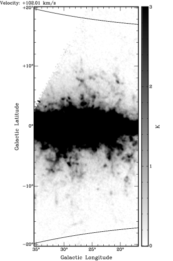
Figure 1.— H I intensity in a single GASS channel at $V_{\mathrm{LSR}}=102$ km s^-1 over the region of the first Galactic quadrant studied here. This area is symmetric in longitude to the fourth quadrant region studied in Paper I and covers the same latitudes. The curved lines show the latitude boundaries of the region searched for clouds. The lack of data in the top, left corner shows the declination limit of GASS.

2.2. The QI Tangent Point Sample

To define a sample of disk-halo clouds that has reasonably well-determined properties, we limited the study of QI clouds to those located near tangent points, where the largest velocity, $V_{\mathrm{t}}$, occurs as the line of sight reaches the minimum Galactocentric radius (see Figure 2). In the absence of random motions, clouds in pure Galactic rotation cannot have $V_{\mathrm{LSR}}>V_{\mathrm{t}}$, and all clouds with $V_{\mathrm{LSR}}=V_{\mathrm{t}}$ would be located at tangent points. However, random motions characterized by a cloud-cloud velocity dispersion ($\sigma_{cc}$) can push a cloud’s $V_{\mathrm{LSR}}$ beyond $V_{\mathrm{t}}$. The deviation velocity, $V_{\mathrm{dev}}\equiv V_{\mathrm{LSR}}-V_{\mathrm{t}}$, is a measure of the discrepancy between a cloud’s LSR velocity and the maximum velocity expected from Galactic rotation in its direction. By focusing on clouds with velocities beyond $V_{\mathrm{t}}$, i.e., with $V_{\mathrm{dev}}\gtrsim 0$ km s^-1 in QI, we isolate a tangent point sample of clouds within a specific region of the Galaxy whose volume is dependent on the cloud-cloud velocity dispersion (Celnik et al., 1979; Stil et al., 2006). Note that because we study clouds only relatively close to the Galactic plane, our definition of $V_{\mathrm{dev}}$ assumes corotation, but, unlike the definition used for studies of high-velocity clouds (Wakker, 1991), does not include presumptions about the thickness of the H I layer.

Figure 2.— Schematic view of the QI and QIV tangent point regions of the Galaxy discussed in this paper. The longitude boundaries of the regions are denoted by the dotted arrows and the locus of tangent points is the dashed circle that connects the Sun and the Galactic center. The solid lines enclose the area around the tangent points bound by the longitude limits and a kinematic distance $\pm 18$ km s^-1 about $V_{\mathrm{t}}$ for a flat rotation curve. Most of the clouds discussed here lie in these two areas.

We define the tangent point sample as those clouds with velocities $V_{\mathrm{LSR}}\geq V_{\mathrm{t}}-0.8$ km s^-1, where $0.8$ km s^-1 accounts for one channel spacing. Clouds that meet this velocity criterion must lie reasonably close to the tangent point, and thus at a distance from the Sun $d_{\mathrm{t}}=R_{0}\cos(l)/\cos(b)$ where $R_{0}\equiv 8.5$ kpc. The accuracy of the adopted distances has been determined using the simulations of §3. Terminal velocities were taken from the analysis of QI H I by McClure-Griffiths & Dickey (in preparation) derived identically to their QIV work (McClure-Griffiths & Dickey, 2007) used in Paper I. At longitudes outside the McClure-Griffiths & Dickey range ($l<19\arcdeg$), terminal velocities were taken from the CO observations of Clemens (1985).

The procedure to detect and measure clouds in the QI tangent point sample is identical to that for QIV and used the following two criteria: (1) clouds must span 4 or more pixels and be clearly visible over three or more channels in the spectra, and (2) clouds must be distinguishable from unrelated background emission. Sample spectra of clouds within QI are shown in Figure 3. Clouds are blended and confused at low $V_{\mathrm{dev}}$ and near the Galactic plane, and they become impossible to identify. We quantify this effect and apply it to our simulations (§3.1). Paper I gives further details on the selection criteria and search method.

Figure 3.— A random selection of spectra showing disk-halo clouds detected in the GASS QI data.

2.3. Observed Properties of the QI Tangent Point Sample

We detect and measure 255 H I tangent point clouds in the QI region. Their properties are presented in Table 1 and include Galactic longitude, $l$, Galactic latitude, $b$, velocity with respect to the local standard of rest, $V_{\mathrm{LSR}}$, peak brightness temperature, $T_{\mathrm{pk}}$, FWHM of the velocity profile, $\Delta v$, peak H I column density, $N_{HI}$, minor and major axes, $\theta_{\mathrm{min}}$ and $\theta_{\mathrm{maj}}$, and the H I mass, $M_{HI}d^{-2}$. These properties were determined analogously to those in Paper I. Histograms of peak brightness temperature, FWHM, and angular size are presented in Figure 4. The clouds have properties similar to those detected in QIV, with median values $T_{\mathrm{pk}}=0.5$ K, $\Delta v=10.6$ km s^-1, and angular size $25^{\prime}$. As many as 80% of the clouds may be unresolved in at least one dimension.

Table 1Observed Properties of Tangent Point H I Clouds in the Quadrant I Region

$l$	$b$	$V_{\mathrm{LSR}}$	$T_{\mathrm{pk}}$	$\Delta v$	$N_{HI}$	$\theta_{\mathrm{min}}\times\theta_{\mathrm{maj}}$	$M_{HI}d^{-2}$
(deg)	(deg)	(km s-1)	(K)	(km s-1)	($\times 10^{19}$ cm-2)	(arcmin $\times$ arcmin)	($M_{\odot}$ kpc-2)
$17.30$	$-8.80$	$135.9\pm 2.6$	$0.84$	$12.5\pm 1.3$	$2.04\pm 0.28$	$16\times 30$	$9.8$
$17.44$	$2.17$	$139.8\pm 4.7$	$0.35$	$14.0\pm 3.0$	$0.95\pm 0.28$	$18\times 21$	$6.2$
$17.60$	$-11.21$	$134.4\pm 4.9$	$0.41$	$16.0\pm 2.9$	$1.27\pm 0.32$	$20\times 22$	$5.1$
$17.72$	$3.94$	$133.6\pm 10.2$	$0.21$	$21.8\pm 7.5$	$0.89\pm 0.44$	$20\times 34$	$8.7$
$17.85$	$-9.66$	$131.7\pm 1.7$	$0.87$	$8.2\pm 1.0$	$1.39\pm 0.21$	$20\times 24$	$7.7$

Note. — Table 1 is published in its entirety in the electronic edition of the Astrophysical Journal. A portion is shown here for guidance regarding its form and content. Properties were determined analogously to those described in Paper I.

Figure 4.— (a) Histogram of peak brightness temperature of the QI tangent point clouds. The median $T_{\mathrm{pk}}=0.5$ K while the lower cutoff is due to the sensitivity limit. The arrow represents the $5\Delta T_{b}$ detection level. We assume $\sqrt{N}$ errors. (b) Histogram of the FWHM of the velocity profile of the tangent point clouds. The median value is $10.6$ km s^-1 and most profiles are well resolved. (c) Histogram of the angular size of the clouds, $(\theta_{\mathrm{maj}}\theta_{\mathrm{min}})^{1/2}$, where $\theta_{\mathrm{maj}}$ and $\theta_{\mathrm{min}}$ are from Table 1. The median angular diameter of the clouds is $25^{\prime}$. The spatial resolution limit of $16^{\prime}$ is noted with the arrow.

Figure 5 shows the longitude vs. $V_{\mathrm{LSR}}$ of all clouds from the tangent point sample within the QI region, along with the adopted terminal velocity curve. Although we searched for clouds at all velocities between $V_{\mathrm{t}}$ and $V_{\mathrm{LSR}}=300$ km s^-1, there were no clouds detected at $V_{\mathrm{LSR}}>160$ km s^-1, and no cloud has a velocity $>50$ km s^-1 beyond that allowed by Galactic rotation. Just as in the QIV data of Paper I, there is a steep decline in the number of clouds beyond the terminal velocity indicating that the kinematics of these clouds are dominated by Galactic rotation.

Figure 5.— Longitude–velocity diagram of clouds with $V_{\mathrm{LSR}}\gtrsim V_{\mathrm{t}}$ (crosses) within the QI region. The terminal velocity curve (solid line) was derived from H I and CO observations near the Galactic plane. The steep decline in the number of clouds with $V_{\mathrm{LSR}}\gg V_{\mathrm{t}}$ (see also Figures 8 and 13) shows that the motions of these clouds are dominated by Galactic rotation. We searched all $V_{\mathrm{LSR}}\leq 300$ km s^-1 but find no clouds with $V_{\mathrm{LSR}}>160$ km s^-1.

2.4. Derived Properties of the QI Tangent Point Sample

In Table 2 we present the cloud properties that depend on the assumption that the clouds are located at tangent points, which include the distance, $d$, Galactocentric radius, $R$, distance from the Galactic plane, $z$, radius, $r$, and physical mass of H I, $M_{HI}$. The deviation velocity, $V_{\mathrm{dev}}\equiv V_{\mathrm{LSR}}-V_{\mathrm{t}}$, is also presented, which shows the discrepancy between a cloud’s LSR velocity and the maximum velocity expected from Galactic rotation in its direction. These properties were determined analogously to those for the QIV clouds as described in Paper I. Errors were also determined analogously, with the uncertainty in the terminal velocity, $\delta V_{\mathrm{t}}$, taken to be $3$ km s^-1 for all clouds at $l>19\arcdeg$, where the terminal velocities were determined from H I observations, and $9$ km s^-1 for longitudes where the terminal velocity was derived from CO observations. These adopted uncertainties are identical to those used in Paper I; the difference between H I and CO uncertainties is expected to account for the granularity of molecular clouds (Burton & Gordon, 1978; McClure-Griffiths & Dickey, 2007). For quantities whose uncertainties depend on distance, a simulated population of clouds was used to determine these effects.

Table 2Derived Properties of Tangent Point H I Clouds in the Quadrant I Region

$l$	$b$	$V_{\mathrm{LSR}}$	$V_{\mathrm{dev}}$	$d$	$R$	$z$	$r$	$M_{HI}$
(deg)	(deg)	(km s-1)	(km s-1)	(kpc)	(kpc)	(kpc)	(pc)	($M_{\odot}$)
$17.30$	$-8.80$	$135.9\pm 2.6$	$5.1\pm 9.4$	$8.2\pm 0.6$	$2.5^{+0.1}$	$-1.26\pm 0.10$	$26\pm 5$	$660\pm 280$
$17.44$	$2.17$	$139.8\pm 4.7$	$6.6\pm 10.2$	$8.1\pm 0.6$	$2.5^{+0.1}$	$0.31\pm 0.02$	$23\pm 4$	$410\pm 180$
$17.60$	$-11.21$	$134.4\pm 4.9$	$2.6\pm 10.3$	$8.3\pm 0.6$	$2.6^{+0.1}$	$-1.61\pm 0.12$	$25\pm 5$	$350\pm 150$
$17.72$	$3.94$	$133.6\pm 10.2$	$1.3\pm 13.6$	$8.1\pm 0.6$	$2.6^{+0.1}$	$0.56\pm 0.04$	$30\pm 6$	$580\pm 250$
$17.85$	$-9.66$	$131.7\pm 1.7$	$3.1\pm 9.2$	$8.2\pm 0.6$	$2.6^{+0.1}$	$-1.38\pm 0.11$	$26\pm 5$	$520\pm 220$

Note. — Table 2 is published in its entirety in the electronic edition of the Astrophysical Journal. A portion is shown here for guidance regarding its form and content. Properties were determined analogously to those described in Paper I.

The distributions of radii and mass of the clouds are shown in Figures 6 and 7. The median radius is $28$ pc while the median mass in H I is $700M_{\odot}$. It is likely that the individual values for the radii are overestimates, as a significant fraction of clouds appear to be unresolved. Confusion of unrelated clouds may also increase the measured angular size of small clouds. We used simulations to interpret the $V_{\mathrm{dev}}$, $z$, and $R$ distributions and present the results in the following section.

Figure 6.— Histogram of physical radius of the QI tangent point clouds. The median radius is $28$ pc. The spatial resolution limit of $16^{\prime}$ at the median cloud distance gives a limiting radius of $18$ pc. We assume $\sqrt{N}$ errors.

Figure 7.— Histogram of the H I mass of the tangent point clouds in the QI data set. The median mass is $\sim 700\ M_{\odot}$. We assume $\sqrt{N}$ errors.

3. Analysis of the QI Tangent Point Sample

3.1. Simulation of the Cloud Distribution

As demonstrated in Paper I, simulations can establish the fundamental characteristics of an observed population, including the uncertainties introduced by the assumption that all clouds with $V_{\mathrm{dev}}\gtrsim 0$, i.e., $V_{\mathrm{LSR}}\gtrsim V_{\mathrm{t}}$, are at the tangent point. Indeed, without simulations it is difficult to accurately derive quantities such as the surface density or scale height from the tangent point cloud data. Consider, for example, a population of clouds in a small area at a tangent point in QI that have a characteristic cloud-cloud velocity dispersion $\sigma_{cc}$. The ensemble has on average $\langle V_{\mathrm{LSR}}\rangle=V_{\mathrm{t}}$, and exactly half of the clouds will have $V_{\mathrm{LSR}}\geq V_{\mathrm{t}}$ and thus be included in the tangent point sample. An area along the line of sight somewhat closer to us than the tangent point will have $\langle V_{\mathrm{LSR}}\rangle<V_{\mathrm{t}}$, but owing to random motions, some fraction of the clouds — fewer than half — will nonetheless have $V_{\mathrm{LSR}}\geq V_{\mathrm{t}}$ and thus end up in the sample of “tangent point” clouds. The number that do depends on the number of clouds at the offset location and the cloud-cloud velocity dispersion. Because the change in $\langle V_{{\mathrm{LSR}}}\rangle$ with distance from the Sun may be only 5-10 km s^-1 kpc^-1 over much of the inner Galactic disk, a very large volume of the Galaxy must be simulated to encompass all clouds likely to end up with forbidden velocities.

By determining the functions that best represent the observed data, an understanding of the properties of the cloud population is obtained that is otherwise unattainable. We simulated a population of clouds to represent the observed tangent point population within QI, applying the same $l$, $b$ and $V_{\mathrm{LSR}}$ selection criteria as for the observed population. A cut was also applied to account for the declination limit of the data. The functional form for the cloud distribution is identical to that adopted for QIV:

$$n(R,z)=\Sigma(R)\exp\left({-\frac{|z|}{h}}\right),$$ (1)

where $\Sigma(R)$ is the surface density in kpc^-2, $h$ is the exponential scale height, and $R$ and $z$ are the cylindrical coordinates. $\Sigma(R)$ is composed of $16$ independent bins of width $0.25$ kpc, spanning $R=2.5$ to $6.5$ kpc.

The velocities of the simulated clouds were derived assuming a flat rotation curve where $\Theta=\Theta_{0}=220$ km s^-1 with a random line of sight component drawn from a Gaussian with a dispersion $\sigma_{cc}$. Corotation is assumed: there is no variation in Galactic rotational velocity with distance from the plane. This issue is discussed in §5.1.3. Over the first and second quadrants, $5\times 10^{4}$ clouds were generated of which 1954 lay within the defined $l$, $b$, $V_{\mathrm{LSR}}$, and $\delta$ range of the QI clouds. This set was then normalized to compare directly with the observed population and Kolmogorov-Smirnov (K-S) tests were performed to estimate the quality of the fit between observation and simulation. Results of the fits to the distributions are presented in §§3.2–3.4. We defer a discussion of the implications of these findings along with a detailed comparison between the first and fourth quadrant clouds until §4.

To determine the uncertainties introduced by the assumption that all clouds with $V_{\mathrm{dev}}\gtrsim 0$ are located at tangent points at a distance $d_{\mathrm{t}}=R_{0}\cos(l)/\cos(b)$, we calculated the fractional distance error of the simulated clouds as a function of deviation velocity, longitude and latitude. As shown by the simulations presented in Paper I, clouds with increasingly forbidden velocities have smaller distance uncertainties, i.e., are more likely to be actually located at $d_{\mathrm{t}}$. This can be understood as follows. The cloud in QI with the highest forbidden velocity has $V_{\mathrm{dev}}\approx 42$ km s${}^{-1}\approx 3\sigma_{cc}$ (see below). From a group of $\sim 100$ clouds at the tangent points with a random velocity of $\sigma_{cc}$ we would expect to find $\sim 1$ such cloud. However, at a location away from the tangent point, where the $\langle V_{\mathrm{LSR}}\rangle$ is much lower, a cloud would have to have a more extreme random velocity, $\gg 3\sigma_{cc}$ to have the identical $V_{\mathrm{dev}}$. Thus the greater the $V_{\mathrm{dev}}$, the more likely, on average, that a cloud has come from a population with high $V_{\mathrm{LSR}}$ and is thus near the tangent point. There is also a slight dependence of the distance uncertainties on longitude, but no dependence on latitude. Likewise, there is a longitude and deviation velocity dependence for the uncertainty in Galactocentric distance.

Confusion effects are a strong function of proximity of clouds to the bulk of Galactic H I: clouds will increasingly be blended and missed at lower heights and lower values of $V_{\mathrm{dev}}$. This is obvious from Figure 1. The confusion manifests itself in the $z$ vs. $V_{\mathrm{dev}}$ plot of Figure 8 as the triangular region near the Galactic plane that is devoid of detected clouds. To account for these effects, we have parameterized the boundaries of the confusion-affected region by the dashed lines shown in Figure 8, and apply these cutoffs to both the observed and simulated data to compare the two as directly as possible. This is in contrast to how we addressed these effects with the QIV data, where we simply omitted all clouds with $|b|\leq 2\arcdeg$, as the number of tangent point clouds in QIV was too small to justify a more detailed cutoff.

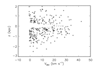
Figure 8.— Distance from the Galactic plane as a function of deviation velocity of QI tangent point clouds. Confusion limits the detectability of clouds that have low values of $V_{\mathrm{dev}}$ and are near the plane. Dashed lines represent the cutoffs that were applied to the simulations to reflect the effects of this confusion. Note the decrease in number of clouds as a function of $V_{\mathrm{dev}}$ at all $z$, showing that the disk-halo clouds follow Galactic rotation.

3.2. Cloud-Cloud Velocity Dispersion

The simulated population of QI clouds that best represents the observed first quadrant population has a random cloud-cloud velocity component drawn from a Gaussian with a dispersion $\sigma_{cc}=14.5$ km s^-1 (with a K-S test probability of $51\%$ that the observed and simulated distributions were drawn from the same distribution). Values of $\sigma_{cc}$ between $14$ and $15.5$ km s^-1 also provide acceptable fits to the measured $V_{\mathrm{dev}}$, having K-S test probabilities $\geq 15\%$.

3.3. Radial Surface Density

The amplitude of each radial bin, $\Sigma(R)$, was optimized to best fit the observed longitude distribution of the tangent point clouds by minimizing the Kolmogorov-Smirnov $D$ statistic (the maximum deviation between the cumulative distributions) using Powell’s algorithm (Press et al., 1992). The fits were optimized for three different initial estimates of $\Sigma(R)$, and as they all converged on a similar solution, we adopted the mean of the three solutions as the best fit to the data.

The longitude distribution of both the observed and simulated population of clouds, along with that derived from a population of clouds with a uniform surface density, is shown in Figure 9. The K-S test probability is 88% that the observed and simulated distributions were drawn from the same distribution. Such an unusually high K-S test probability is not surprising in this case, as the parameters of the simulation were fine-tuned to reproduce the observed longitude distribution. The probability that the observed and a uniformly distributed population were drawn from the same distribution is $3\%$, so the observations are marginally inconsistent with being drawn from a population of clouds with a uniform surface density. In this case most of the discrepancy arises from the bins with the highest longitude.

Figure 9.— Longitude distribution of observed (solid line) and simulated (dashed line) QI clouds, with a uniform surface density population overlaid (dotted line). The uniformly distributed population of clouds closely resembles the observed population except at the highest longitudes, suggesting that the tangent point clouds within the QI region are distributed rather evenly. We assume $\sqrt{N}$ errors.

The most likely radial surface density distribution is shown in Figure 10. Although the area we studied included tangent points only over $2.5\leq R\leq 4.9$ kpc, the simulations indicate that a few clouds at larger $R$ are expected to have random velocities that, when added to their rotational velocity, give them a $V_{\mathrm{LSR}}>V_{\mathrm{t}}$ and thus place them in the tangent point sample.

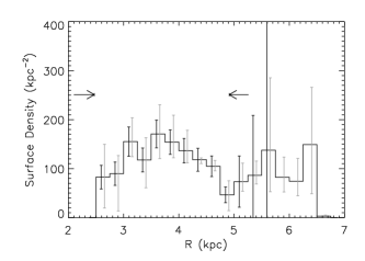
Figure 10.— Radial surface density distribution of the simulated population of QI clouds. The black error bars represent the Poisson error in the number of clouds expected to fall into the observed sample, which determined the ability of the observed data to constrain the simulated distribution. The grey error bars represent the range in values for the 3 different starting points used in the minimization. Error bars are large in the right-most bins because very few clouds at these radii have high enough random velocities such that their $V_{\mathrm{LSR}}>V_{\mathrm{t}}$. No simulated clouds within the largest radial bins meet the selection criteria of the tangent point sample. The bins without black error bars are therefore unconstrained by the observed cloud population. Arrows represent the tangent points at the longitude boundaries of the QI region.

3.4. Vertical Distribution

The vertical distribution of the tangent point clouds is best represented by an exponential with a scale height $h=800$ pc (see Figure 11). Because K-S tests are most sensitive to the differences near the median of the distribution, we tested both $n(b)$ and $n(|b|)$: the former gives higher weight to clouds closer to the plane, while the latter weighs more highly the higher latitude clouds. Also, fitting to $n(b)$ is sensitive to symmetries about the plane while fitting to $n(|b|)$ is not. For $h=800$ pc, the K-S test probability that the observed and simulated clouds were drawn from the same vertical function is $61\%$ when comparing against $|b|$, but not acceptable when comparing against $b$. Scale heights between $700$ and $850$ pc were acceptable for the distribution of $|b|$, while scale heights between 950 and $1100$ pc were consistent with the distribution of $b$ values, with 1000 pc being the best fit, having a probability of $24\%$. This discrepancy likely indicates that our low-latitude confusion cutoff (Figure 8) is not conservative enough. As this effects the distribution of $b$ more strongly than of $|b|$, we adopt the preferred value from the latter comparison, $h=800$ pc.

Figure 11.— Vertical distribution of the observed QI (solid line) and simulated (dashed line) population of clouds. The observed population is well represented by a simulated population with an exponential scale height of $800$ pc. Note that inclusion of a simulated “confusion-cutoff” (Figure 8) does a reasonable job of reproducing the decrease of clouds near the plane. We assume $\sqrt{N}$ errors.

4. Comparison of Cloud Populations in the Two Quadrants

4.1. Trends in Physical Properties

The physical properties of disk-halo tangent point H I clouds from QI and QIV are summarized in Table 3. Individual clouds in both quadrants of the Galaxy have similar properties, which suggests that they belong to the same population and probably have similar origins and evolutionary histories. We defer an analysis of the physical properties of the clouds to another paper; here we note just a few trends that give important insight into the nature of the disk-halo clouds.

Table 3Properties of Tangent Point Disk-Halo Clouds in GASS

	Median		90% Range
Parameter	QI	QIV	QI	QIV
$T_{\mathrm{pk}}$ (K)	$0.5$	$0.5$	$0.2\rightarrow 2.7$	$0.2\rightarrow 2.1$
$\Delta v$ (km s-1)	$10.6$	$10.6$	$4.2\rightarrow 23.2$	$4.4\rightarrow 22.3$
$N_{HI}$ ($\times 10^{19}$ cm-2)	$1.0$	$1.0$	$0.2\rightarrow 6.2$	$0.3\rightarrow 6.5$
Angular Size (′)	$25$	$28$	$17\rightarrow 38$	$21\rightarrow 44$
$r$ (pc)	$28$	$32$	$<19\rightarrow 44$	$<23\rightarrow 50$
$M_{HI}$ ($M_{\odot}$)	$700$	$630$	$130\rightarrow 4100$	$120\rightarrow 4850$
$d$ (kpc)	$7.7$	$7.7$	$7.2\rightarrow 8.1$	$7.2\rightarrow 8.1$
$R$ (kpc)	$3.7$	$3.6$	$2.7\rightarrow 4.6$	$2.9\rightarrow 4.6$
$|z|$ (pc)	$660$	$560$	$190\rightarrow 1640$	$320\rightarrow 1690$

Note. — Median values of the tangent cloud properties, where the number of tangent point clouds is 255 for QI and 81 for QIV. Most properties have a large scatter about the median in all samples, as demonstrated by the $90\%$ range. The angular size is $(\theta_{\mathrm{maj}}\theta_{\mathrm{min}})^{1/2}$.

First, as the gas mass required for a cloud to be gravitationally bound is $M\approx r\Delta v^{2}/G$, where $r$ is the radius, $\Delta v$ is the FWHM, and $G$ is the gravitational constant, the clouds fail to be self-gravitating by several orders of magnitude. This was noted in the discovery of the disk-halo cloud population, and applies not only to individual clouds, but also to dense clumps within clouds revealed in high-resolution observations (Lockman, 2002; Pidopryhora et al., 2009).

Second, there is strong evidence that clouds farther from the Galactic plane have larger linewidths than clouds nearer the plane (Figure 12). This confirms previous suggestions of the trend (Lockman, 2002; Stil et al., 2006; Ford et al., 2008). Moreover, given its continuity with $|z|$, it does not appear to arise from the superposition of separate populations of clouds, but supports the hypothesis that it reflects pressure variations throughout the halo and the fundamental role that pressure has in controlling the phases of the neutral ISM (Wolfire et al., 1995; Koyama & Ostriker, 2009). Indeed, many clouds at $|z|\sim 1$ kpc exhibit a two-phase structure with broad and narrow line components (Lockman & Pidopryhora, 2005).

Figure 12.— FWHM of the H I profile, $\Delta v$, as a function of distance from the Galactic plane for all tangent point clouds from QI and QIV (crosses). The star at $|z|=0.1$ kpc and $\Delta v=5.5$ km s^-1 shows the median values from the Stil et al. (2006) sample of clouds near the Galactic plane. Linewidths tend to increase with distance from the Galactic plane.

The clouds must be either pressure-confined or transitory features, as they are not gravitationally bound. Without higher resolution data than those presented here, we are unable to measure the pressure of the clouds, so cannot comment directly on the first possibility. If they are transitory features, however, their lifetimes must be significantly less than both the thermal evaporation timescale, which is $\gtrsim 100$ Myr (Stanimirović et al., 2006) and the internal dynamical time ($\sim 3$ Myr for the median cloud radius and linewidth). While the first of these timescales is consistent with them evolving on a free-fall timescale ($\sim 30$ Myr from 1 kpc, based on the vertical potential of Benjamin & Danly 1997), as might be expected if they are lifted or ejected into the halo from the disk or if they form above the disk and rain down, they expand and disperse much more quickly unless there is some form of confinement.

4.2. Cloud Location and Numbers

A summary of the properties of disk-halo H I clouds at the QI and QIV tangent points is presented in Table 4. Although the first and fourth quadrant regions span the same Galactocentric radii and vertical distances from the plane, differing only by being located on opposite sides of the Sun-center line, there is a striking difference in the number of detected tangent point clouds: 255 in QI compared to only 81 in QIV.

Table 4Summary of Disk-Halo H I Cloud Distributions in QI and QIV

	QI		QIV
Parameter	Value	Best Fit	Value	Best Fit	Consistent?
$n_{\mathrm{tp}}$	$255$		$81$		No
$\sigma_{cc}$ (km s-1)		$14-15.5$		$16-22$	Yes
$h$ (pc)		$700-850$		$300-500$	No
$\Sigma(R)$		$\sim$uniform		$\sim$concentrated	No

Note. — The quantity $n_{\mathrm{tp}}$ is the number of clouds detected at the tangent points. Properties derived from simulations are also presented. The number of clouds is strikingly different between quadrants, as are the vertical scale heights and radial surface density distributions. The cloud-cloud velocity dispersions, however, are similar in both quadrants.

Values of $V_{\mathrm{dev}}$ for clouds in QI and QIV are similar (Figure 13), with a K-S probability of $76\%$ of having been drawn from the same distribution, suggesting that the cloud-cloud velocity dispersion in both quadrants is identical. This conclusion is supported by the simulations, which are consistent with $\sigma_{cc}\approx 16$ km s^-1 in both quadrants. The cloud distributions, however, differ significantly in both the vertical and radial directions.

Figure 13.— Distribution of observed $V_{\mathrm{dev}}$ for the QI tangent point clouds (solid line) and the symmetric $-V_{\mathrm{dev}}$ for the QIV clouds (dashed line). The K-S probability is $76\%$ of them having been drawn from the same distribution, and suggests that the cloud-cloud velocity dispersion in both quadrants is identical. This is supported by the simulations, which show that both populations have distributions consistent with $\sigma_{cc}=16$ km s^-1. We assume $\sqrt{N}$ errors.

4.3. Vertical Distribution of Disk-Halo H I Clouds

The vertical distributions of the tangent point clouds derived from the simulations are shown in Figure 14. These distributions properly account for selection effects that artificially skew the appearance of the observed distributions, particularly near the plane. The scale heights differ between quadrants, with $h=400$ pc in QIV compared with $h=800$ pc in QI, as do the acceptable ranges of the scale height: in QIV acceptable fits range from $h=300$ to $500$ pc while in QI acceptable fits are between $h=700$ and $850$ pc. We tested to see if this result could occur because of differences in confusion or asymmetries about the plane, but find it quite robust: there is no overlap in acceptable ranges of $h$ between the QI and QIV tangent point cloud samples.

Figure 14.— Comparison of the derived vertical distributions of disk-halo H I clouds in QI (solid line) and QIV (dashed line) after taking into account selection criteria and confusion. Both distributions are well represented by an exponential, but with a scale height of $h=800$ pc in QI and only $h=400$ pc in QIV.

The origin of the scale height is unclear. If the clouds have a vertical random motion equal to their line of sight random motion, i.e. $\sigma_{z}=\sigma_{cc}$, their scale height at $R\approx 4$ kpc would be less than 100 pc. To achieve their observed distances from the plane at $R=3.8$ kpc the clouds would have to have $\sigma_{z}>60$ km s^-1 in QIV and $>95$ km s^-1 in QI in the model potential of Kalberla et al. (2007). Thus, given that $\sigma_{cc}$ is essentially identical in both quadrants, not only is it impossible for the derived vertical scale height of clouds to arise from motions with a magnitude of the cloud-cloud velocity dispersion $\sigma_{cc}$, but $\sigma_{cc}$ cannot be connected to the scale height. We will discuss likely explanations for the scale height in a later section.

4.4. Radial Surface Density

The radial surface density of clouds derived from the simulations, $\Sigma(R)$, is given in Figure 15. It shows not only the much larger number of clouds in QI than in QIV, but that the shape of the distributions are fundamentally different. The surface density in QI is relatively uniform, while the surface density in QIV is concentrated, and declines rapidly at $R>4.2$ kpc. The difference is statistically robust. We have compared the shapes of $\Sigma(R)$ within the well-constrained $2.5\leq R\leq 5$ kpc bins of the two quadrants, rescaling them to have the same number of clouds so as to compare only the shape, by calculating the $\chi^{2}$ of their difference compared to the null hypothesis that the shapes are identical. The null hypothesis is strongly ruled out with $\chi^{2}=31.5$ over 10 degrees of freedom, or a probability of $0.05\%$.

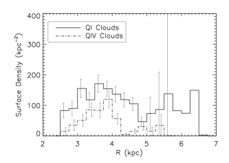
Figure 15.— Comparison of the derived radial surface density distribution of disk-halo H I clouds within the QIV region (dashed-dot line) and the QI region (solid line). There are $\approx 3$ times as many disk-halo clouds at the tangent points in QI as in QIV, and the radial distributions differ significantly as well. Error bars denote the Poisson error in the number of clouds expected to fall into each bin. The right-most bins have no error bars because no clouds at these $R$ are expected to meet the criteria of the tangent point sample. These bins are therefore unconstrained by the observed cloud population.

5. Origin of the QI-QIV Asymmetries

Even though the individual disk-halo H I clouds have virtually identical properties in the two quadrants, there are three major asymmetries in the populations: 1) There are three times as many clouds in the QI volume as in the identical volume of QIV. 2) The scale height of the QI clouds is twice that of QIV clouds. 3) The radial surface density distributions are not at all alike. In this section we consider possible explanations for these differences.

5.1. Selection Effects

5.1.1 Instrumental Effects, Cloud Selection, Confusion

The GASS H I data set has uniform instrumental properties. Although the QIV clouds were measured from an early version of the data it differs little from the final version, and in no significant way that would produce a large discrepancy between QI and QIV. One of us (H. A. F.) developed the cloud identification and measurement techniques, and produced the cloud catalogues. Every attempt was made to apply the selection criteria uniformly to the two regions. The strongest evidence for a lack of bias in the cloud selection process is given by the near identity of individual cloud properties in the two regions. This is apparent from Table 3, and also from Figures 16 and 17, which show that the distribution of peak line intensity and cloud mass is essentially identical for the tangent point clouds in QI and QIV. If there were differences in the detection level or noise in the two data sets we would expect to see, for example, more clouds with small $T_{\mathrm{pk}}$ or small H I masses in QI. This does not occur. We conclude that changes in survey sensitivity, or cloud identification and selection criteria, are not the source of the QI-QIV differences.

One difference between the QI and QIV data is that the area surveyed in QI is $\sim 15\%$ smaller due to the declination limit of GASS (see Figure 1). However, this will only cause us to underestimate the difference in the number of clouds. We note that our simulations take this effect into account and the radial surface densities, vertical distributions, and cloud-cloud velocity dispersions are therefore all unaffected.

Near the Galactic plane, or at low values of $|V_{\mathrm{dev}}|$, clouds blend with each other and with unrelated emission making it impossible to identify and measure them. It is conceivable that the cloud population in QI is less confused than in QIV, allowing more clouds to be detected. If, for example, the QI clouds had a larger $\sigma_{cc}$ than the QIV clouds then more of them would lie at V${}_{LSR}>V_{t}$ where they might be less confused with unrelated H I. This might also give an apparent increase in scale height. Table 4 shows, however, that $\sigma_{cc}$ is nearly identical in the two regions and if anything, is somewhat smaller in QI than in QIV. Moreover, Figure 18 shows that there are more clouds observed in QI at nearly every distance from the Galactic plane, whereas confusion is important only at $|z|\lesssim 0.5$ kpc. Confusion cannot be the source of the QI-QIV differences.

Figure 16.— Comparison of the normalized distribution of observed peak line temperatures in the QI (solid line) and QIV (dashed line) tangent point cloud samples. The sensitivity limits in QI and QIV are identical.

Figure 17.— Comparison of the normalized distribution of cloud masses in the QI (solid line) and QIV (dashed line) tangent point cloud samples. There is no bias toward lower mass clouds in QI.

Figure 18.— Comparison of the observed distance from the plane of H I clouds in the QI (solid line) and QIV (dashed line) tangent point samples. There are more clouds in QI than QIV at virtually every distance from the plane, eliminating any variation in confusion as a source of the QI-QIV differences.

5.1.2 Kinematic Selection Effects

The QI tangent point clouds were chosen from those with $V_{\mathrm{LSR}}\gtrsim V_{\mathrm{t}}$, where $V_{\mathrm{t}}$ is derived at each longitude from measurements of H I or CO made close to the Galactic plane. Different authors use different methods to derive $V_{\mathrm{t}}$, and we were careful to use values that treat both quadrants uniformly (see §2.2). Our adopted values of $V_{\mathrm{t}}$ are shown in Figure 19. The QI values lie below those of QIV at about half of the longitudes. The existence of large-scale deviations from symmetry in the terminal velocities (and possibly in the rotation curve itself) was an early discovery of Galactic H I studies (Kerr, 1962), and the reason that we chose to use measured values of $V_{\mathrm{t}}$ to derive the cloud samples rather than a theoretical rotation curve. Nonetheless, it is true that if for some reason the kinematics of the disk-halo cloud population is actually symmetric about the Galactic center, our choice of an asymmetric $V_{\mathrm{t}}$ curve would artificially inflate the number of clouds in QI compared to QIV.

Could this be the cause of the differences we detect? To explore this we have calculated the number of QIV tangent point clouds that would be found if the QI rather than the QIV form of $V_{\mathrm{t}}$ were used. This change would increase the number of QIV tangent point clouds from 81 to 130, still a factor of two fewer than in QI. In another test, we selected clouds in QI using for $V_{\mathrm{t}}$ at each longitude the maximum value from Figure 19. This lowered the number of clouds in the QI sample from 255 to 180, but still left it at twice the number as in QIV.

To make the number of tangent point clouds equal in QI and QIV would require the values of $V_{\mathrm{t}}$ to be systematically in error by $>20$ km s^-1 over at least $20\arcdeg$ of longitude in one quadrant only. Levine et al. (2008) have independently derived terminal velocities from H I data over part of the longitude range of interest. Their values have, on average, a lower magnitude than those we use, reflecting a difference in the adopted definition of $V_{\mathrm{t}}$. Nonetheless, their analysis shows an asymmetry similar to that in Figure 19, and an average difference between QI and QIV similar to the values we use.

We conclude that the difference in the disk-halo tangent point cloud sample between QI and QIV is highly unlikely to arise from kinematic selection effects. It is important to note as well that simply equalizing the numbers of clouds in the two quadrants does not remove the substantial difference in scale height (Figure 14) or radial distribution (Figure 15). We can find nothing in our observations or analysis that would erroneously create differences of the observed magnitude.

Figure 19.— Adopted terminal velocity curves for QI and QIV. In QI, the terminal velocities were taken from the analysis of H I by McClure-Griffiths & Dickey (in preparation). At longitudes outside the McClure-Griffiths & Dickey range ($l<19\arcdeg$), terminal velocities were taken from the CO observations of Clemens (1985). In QIV, the terminal velocities were taken from the analysis of H I by McClure-Griffiths & Dickey (2007), while for $l\geq 339\fdg 7$ we used terminal velocities determined by Luna et al. (2006).

5.1.3 The Assumption of Corotation

Throughout this work we have assumed that there is no dependence of the Galactic rotation curve on distance from the Galactic plane. Other galaxies, however, show evidence for a systematic lag in rotation of $10$–$20$ km s^-1 kpc^-1 in both ionized and neutral gas that begins perhaps 1 kpc from the plane and is of unknown origin (Fraternali et al., 2005; Rand, 2005; Marinacci et al., 2010). Evidence for departures from corotation in the Milky Way is scant (Pidopryhora et al., 2007). We defer a full analysis to a subsequent paper, but note that because most of the clouds discussed here lie at $|z|<1$ kpc, a lag may be difficult to detect. If a significant number of the disk-halo clouds do lag somewhat behind Galactic rotation, then our analysis has underestimated their numbers at the tangent point, with the result that the true scale height, and the true surface density, will be larger than given here, especially in QI where the population extends much farther from the plane than in QIV.

5.2. Differences Caused by Galactic Structure

Given that the difference in the numbers, scale height and surface density are real, might they be carrying information on some large-scale feature of the Milky Way? Figure 20 suggests that this is the case. It shows an idealization of the Galaxy with the outline of the regions of the first and fourth quadrants from which the tangent point clouds are selected (Figure 2). This depiction of the Galaxy incorporates recent findings from the Galactic Legacy Infrared Mid-Plane Survey Extraordinaire (GLIMPSE; Benjamin et al. 2003), a survey that was conducted using the Spitzer Space Telescope. The GLIMPSE data suggest that the spiral structure of the Galaxy, which had originally been thought to consist of four major arms, is dominated by two arms (the Scutum-Centaurus and Perseus arms) that extend from each end of a central bar. There are also two minor arms (the Norma and Sagittarius arms), located between the major arms. The artist’s conception incorporates the GLIMPSE findings on the location of the bar and spiral arms (Benjamin et al., 2005), as well as recent VLBI determinations of parallactic distance to some H II regions (e.g., Reid et al. 2009), the discovery of the far side of the 3-kpc arm (Dame & Thaddeus, 2008), and other evidence relevant to the overall pattern of star formation in the Galaxy (R. A. Benjamin, private communication). The solid lines enclose areas within the longitude limits of our study, with a line of sight extent equivalent to $|V_{\mathrm{LSR}}|=|V_{\mathrm{t}}|-18$ km s^-1, i.e. the $\sim 1\sigma$ volume around the tangent point for a flat rotation curve.

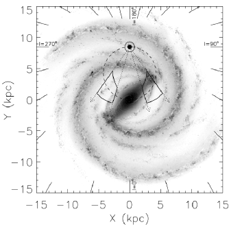
Figure 20.— Artist’s conception of the Milky Way as derived from GLIMPSE survey infrared data. The longitude boundaries of the QI and QIV regions are denoted by the dotted arrows while the locus of tangent points is represented by the dashed circle. The solid lines enclose the area around the tangent points bound by our longitude limits and a kinematic distance $\pm 18$ km s^-1 away from $V_{\mathrm{t}}$ from Figure 2. The two regions studied here, though selected to be symmetric with respect to the Sun-center line, actually sample two very different parts of the Galaxy. The QI area covers the near tip of the Galactic bar where a major spiral arm originates, while the QIV area contains only a minor arm. The artist’s conception image is from NASA/JPL-Caltech/R. Hurt (SSC-Caltech).

In the GLIMPSE view of the Milky Way, the QIV tangent point region covers a rather sparse section of the Galaxy through which only a segment of the minor Norma spiral arm passes, while the QI region lies on a much richer portion of the Galaxy where the near end of the Galactic bar merges with the beginning of the major Scutum-Centaurus arm. The radial surface density distributions of the disk-halo clouds mirror the spiral structure in both regions, suggesting a relation between the clouds and spiral features. The association of the disk-halo clouds with regions of star formation, and specifically with the asymmetry caused by the Galactic bar, offers the only solution we can find to the asymmetries in the disk-halo cloud distributions.

There is observational evidence that there has been a significant burst of star formation near where the Scutum-Centaurus arm meets the end of the bar, in the form of observations of multiple red supergiant clusters in the area ($l\sim 29\arcdeg$; e.g., see Figer et al. 2006; Davies et al. 2007; Alexander et al. 2009; Clark et al. 2009). Motte et al. (2003) even suggest that the H II region complex W43, located at $l\sim 31\arcdeg$, is a “ministarburst.” Other galaxies also have increased star formation occurring where spiral arms meet the bar ends (Phillips, 1993). We find a plethora of disk-halo H I clouds in the region where the Scutum-Centaurus arm extends from the bar end in the first quadrant, three times more than in the fourth quadrant region, suggesting that the number of clouds and their scale heights are proportional to the amount of star formation.

We can, however, find no detailed correlation between disk-halo clouds and other tracers of star formation. Neither molecular clouds (Bronfman et al., 1988), nor HII regions (Paladini et al., 2004), show a strong QI-QIV asymmetry like the disk-halo clouds, or have a radial surface density distribution with a similar shape. Methanol masers detected in the 6.7 GHz emission line are known tracers of high-mass star formation (Xu et al., 2008), and some are formed in very early protostellar cores (Minier et al., 2005). Methanol masers that have been detected by Pestalozzi et al. 2005; Pandian et al. 2007; Ellingsen 2007; Xu et al. 2008 and Cyganowski et al. 2009 within $\pm 30$ km s^-1 of $V_{\mathrm{t}}$ show a factor 2.2 excess in the QI region compared with QIV, not as large as the factor of 3.2 difference in disk-halo H I clouds, but larger than in any other population of which we are aware. However, the maser numbers peak at longitudes $\sim 30\arcdeg$ on either side of the Galactic center, a distribution not at all like the tangent point H I clouds.

We conclude that the numbers of disk-halo clouds correlate with the amount of star formation on the largest scales, but not with tracers of star formation in detail.

6. Fraction of Galactic Extraplanar H I in Disk-Halo Clouds

The new data allow estimation of the fraction of the total extraplanar H I that is in the form of the disk-halo clouds, through comparison with previous derivations of $n_{HI}(z)$ in the inner Galaxy (we cannot use the current release of GASS data to estimate $n_{HI}(z)$ as these data have not been corrected for stray radiation). Over the first longitude quadrant, Dickey & Lockman (1990) fit the vertical distribution of H I along the tangent points with a three-component model, one of which is an exponential with a scale height of 400 pc. This component contains $1.6\times 10^{20}$ cm^-2 through a full disk. There are about 100 QI disk-halo clouds per kpc² (Figure 10), which at a median H I mass of 700 $M_{\odot}$ sums to $10^{19}$ cm^-2 through a full disk, only about 5% of the total $N_{HI}$ in the Dickey & Lockman (1990) exponential component. The cloud counts, however, are very deficient near the plane because of confusion, and the total number of disk-halo clouds could be 2-3 times larger than we are able to identify. Even so, it appears that the discrete disk-halo H I clouds identified in the GASS data account for no more than perhaps 10-20% of all H I far from the plane in QI.

There are many H I structures above the disk which did not fit our strict criteria for inclusion in the catalog of “clouds” but which still contain significant amounts of H I. Also, there are certainly many small clouds detected at higher resolution (Lockman, 2002) but missed in the GASS study. The existence and extent of a truly diffuse H I halo component in the inner Galaxy thus remains uncertain. This topic will be addressed in a subsequent work when the GASS survey data corrected for stray radiation becomes available.

7. Disk-Halo Clouds as the Product of Stellar Feedback and Superbubbles

In Paper I we suggested that the disk-halo clouds could be a result of superbubbles and material that has been pushed up from the disk, as the presence of many loops and filaments were clearly visible within the QIV data, and many clouds appeared to be associated with these structures. Superbubbles can lift significant amounts of disk gas several kpc into the halo (de Gouveia Dal Pino et al., 2009). They are quite common in areas of star formation (Kalberla & Kerp, 2009), so the presence of such structures would also be expected in the QI region. The Ophiuchus superbubble is an excellent example of such a structure: it is an old superbubble ($\sim 30$ Myr) that lies within the first quadrant region and is above a section of the Galaxy containing many H II regions, including W43 (Pidopryhora et al., 2007). This superbubble is at a distance of $\sim 7$ kpc and is capped by a plume of H I at $\sim 3.4$ kpc above the plane. Many H I features have been observed to be affiliated with this superbubble at velocities near those expected at tangent points, including gas that has been swept up sideways from the disk, and clouds (Pidopryhora et al., 2007, 2009). It is likely some of the tangent point clouds in the first quadrant region are associated with this superbubble.

In §5.2 we suggested that the radial surface density distributions of the disk-halo clouds closely mirrors the spiral structure of the Galaxy, and in particular the asymmetry caused by the Galactic bar. It is interesting to note that extraplanar gas in some external spiral galaxies, such as NGC 4559, appears to be spatially related to star formation activity (Barbieri et al., 2005). Also, the presence of extraplanar dust in external galaxies implies that if extraplanar gas is a result of feedback, the processes transporting the material from the disk must be gentle and likely have low velocities in order for the dust grains to survive (Howk, 2005). This is consistent with the low $\sigma_{cc}$ that we derive for the disk-halo clouds in both quadrants.

Based on the results from our comparisons of the QI and QIV tangent samples, we therefore propose the following scenario for the origin and evolution of halo H I clouds: the clouds are related to areas of star formation, where stellar winds and supernova activity sweep and push gas from the disk into the lower halo. Some neutral gas resides in the walls of superbubbles, whose shells eventually fragment into clouds. As star formation is abundant in spiral arms, the clouds are naturally correlated with the spiral structure of the Galaxy. However, as the timescale for formation of a superbubble ($\sim 20$–$30$ Myr; de Avillez & Breitschwerdt 2004; McClure-Griffiths et al. 2006) is large compared to the lifetime of a star-forming region ($\sim 0.1$ Myr; Prescott et al. 2007), clouds that are produced in shells may no longer be at the same locations as the sites where high-mass stars are forming at the present day. The scale heights of the cloud population are reasonable if the gas is brought into the lower halo by superbubbles or feedback, as high vertical velocities are not required. The magnetic field lines in a supershell are compressed (e.g., Ferrière 2001), which increases the magnetic pressure and may aid in cloud stability if the clouds are related to supershells.

It is important to contrast this scenario with that of a standard galactic fountain, which proposes that clouds are formed by the cooling and condensing of hot gas that has been expelled from the disk, which then falls back towards the plane (Shapiro & Field, 1976; Bregman, 1980). While this model has similarities to our proposed scenario, an important difference is that the distribution of clouds would not be expected to have small-scale features, such as a peaked radial distribution, or a dramatic difference in the number of clouds between different regions of the Galaxy at similar radii, as the hot gas from which they condense is expected to be fairly uniform in the halo (Bregman, 1980). Such features are clearly present in the disk-halo H I cloud distributions, which argues for a scenario where clouds are produced more directly by events occurring within spiral arms. There is also no reason to expect the clouds to be associated with loops and filaments if related to a galactic fountain, but these structures are often observed.

In recent years the definition of a galactic fountain has been expanded to include not just the classical fountain but any scenario where gas is expelled from the disk into the lower halo and later returns to the disk regardless of gas phase and temperature (e.g., see Spitoni et al. 2008). Our proposal falls under this broader categorization of a galactic fountain.

8. Summary Comments

A total of 255 disk-halo H I clouds, some $>2$ kpc from the plane, were detected at the tangent points in the first quadrant region of GASS data, a region in longitude, latitude and velocity that is symmetric to the fourth quadrant region studied in Paper I. Individual cloud properties in the QI sample are very similar to those in the QIV sample, having median values $T_{\mathrm{pk}}=0.5$ K, $\Delta v=10.6$ km s^-1, $r=28$ pc and $M_{HI}=700M_{\odot}$. The clouds do not have enough mass to be self-gravitating. They must either be pressure-confined or transitory. The observed increase in linewidth with distance from the plane suggests that the clouds are pressure-confined and that the linewidths reflect pressure variations throughout the halo.

The cloud-cloud line of sight velocity dispersion is also similar in both regions, with a value $\sigma_{cc}\approx 16$ km s^-1. However, the QI clouds have twice the exponential scale height as the QIV clouds ($h=800$ pc vs. $h=400$ pc). As with the QIV sample, this is many times larger than can be supported by vertical motions with the magnitude of the cloud-cloud line of sight velocity dispersion. Thus the scale height in the two quadrants is neither derived from nor even related to the measured velocity dispersion of the cloud population.

Both the cloud numbers and their Galactic distribution are also markedly different between the two regions, with three times as many clouds being detected in QI than in QIV. As the clouds were selected from a uniform data set using identical criteria, this difference between the regions must result from a fundamental asymmetry between the two parts of the Galaxy. We believe that the differences arise from the coincidental location of the QI sample on a region where a major spiral arm merges with the tip of the Galactic bar, whereas the QIV sample encompasses only a portion of a minor spiral arm. While there is no agreement in detail between the Galactic distributions of disk-halo H I clouds and H II regions, methanol masers, or molecular clouds, we believe that a link with large-scale star forming regions is the only explanation for the extreme difference in numbers, distribution and scale height of clouds in the two regions.

The most likely scenario is that the disk-halo H I clouds are related to areas of star formation and result from stellar feedback and superbubbles that have swept gas into the halo forming (or releasing) the clouds in situ. These events occur frequently within spiral arms, but take tens of Myr to reach their maximum extent, by which time the stellar clusters that produced them are no longer active in star formation. Simulations of superbubble expansion (e.g., Melioli et al. 2008; Ford et al., in preparation) and semi-analytic models (e.g., Spitoni et al. 2008) show that this is a viable mechanism for producing H I clouds in the lower halo.

Disk-halo H I clouds are abundant in both QI and QIV, a volume of many kpc³. They are not an isolated phenomenon, but a major component of the Galaxy. The properties of the disk-halo cloud population rule out the possibility that most of the clouds are created through tidal stripping of satellite galaxies or infalling primordial gas — the clouds are clearly a disk population, concentrated toward the plane, highly coupled to Galactic rotation, and correlated with the spiral structure of the Galaxy. The disk-halo H I clouds therefore play an important role in Galaxy evolution and the circulation of gas between the disk and halo, and are likely common in many external galaxies, though the angular resolution and sensitivity limits of current instruments would make their detection difficult.

References

- Alexander et al. (2009) Alexander, M. J., Kobulnicky, H. A., Clemens, D. P., Jameson, K., Pinnick, A., & Pavel, M. 2009, AJ, 137, 4824
- Audit & Hennebelle (2005) Audit, E., & Hennebelle, P. 2005, A&A, 433, 1
- Baker & Burton (1975) Baker, P. L., & Burton, W. B. 1975, ApJ, 198, 281
- Barbieri et al. (2005) Barbieri, C. V., Fraternali, F., Oosterloo, T., Bertin, G., Boomsma, R., & Sancisi, R. 2005, A&A, 439, 947
- Benjamin et al. (2003) Benjamin, R. A. et al. 2003, PASP, 115, 953
- Benjamin et al. (2005) Benjamin, R. A. et al. 2005, ApJ, 630, L149
- Benjamin & Danly (1997) Benjamin, R. A., & Danly, L. 1997, ApJ, 481, 764
- Bregman (1980) Bregman, J. N. 1980, ApJ, 236, 577
- Bronfman et al. (1988) Bronfman, L., Cohen, R. S., Alvarez, H., May, J., & Thaddeus, P. 1988, ApJ, 324, 248
- Burton & Gordon (1978) Burton, W. B., & Gordon, M. A. 1978, A&A, 63, 7
- Celnik et al. (1979) Celnik, W., Rohlfs, K., & Braunsfurth, E. 1979, A&A, 76, 24
- Clark et al. (2009) Clark, J. S., Negueruela, I., Davies, B., Larionov, V. M., Ritchie, B. W., Figer, D. F., Messineo, M., Crowther, P. A., & Arkharov, A. A. 2009, A&A, 498, 109
- Clemens (1985) Clemens, D. P. 1985, ApJ, 295, 422
- Cyganowski et al. (2009) Cyganowski, C. J., Brogan, C. L., Hunter, T. R., & Churchwell, E. 2009, ApJ, 702, 1615
- Dame & Thaddeus (2008) Dame, T. M., & Thaddeus, P. 2008, ApJ, 683, L143
- Davies et al. (2007) Davies, B., Figer, D. F., Kudritzki, R.-P., MacKenty, J., Najarro, F., & Herrero, A. 2007, ApJ, 671, 781
- de Avillez & Breitschwerdt (2004) de Avillez, M. A., & Breitschwerdt, D. 2004, A&A, 425, 899
- de Gouveia Dal Pino et al. (2009) de Gouveia Dal Pino, E. M., Melioli, C., D’Ercole, A., Brighenti, F., & Raga, A. C. 2009, in Revista Mexicana de Astronomia y Astrofisica Conference Series, Vol. 36, Revista Mexicana de Astronomia y Astrofisica Conference Series, 17–24
- Dedes & Kalberla (2010) Dedes, L., & Kalberla, P. W. M. 2010, A&A, 509, 60
- Dickey & Lockman (1990) Dickey, J. M., & Lockman, F. J. 1990, ARA&A, 28, 215
- Ellingsen (2007) Ellingsen, S. P. 2007, MNRAS, 377, 571
- Ferrière (2001) Ferrière, K. M. 2001, Reviews of Modern Physics, 73, 1031
- Figer et al. (2006) Figer, D. F., MacKenty, J. W., Robberto, M., Smith, K., Najarro, F., Kudritzki, R. P., & Herrero, A. 2006, ApJ, 643, 1166
- Ford et al. (2008) Ford, H. A., McClure-Griffiths, N. M., Lockman, F. J., Bailin, J., Calabretta, M. R., Kalberla, P. M. W., Murphy, T., & Pisano, D. J. 2008, ApJ, 688, 290
- Fraternali et al. (2005) Fraternali, F., Oosterloo, T. A., Sancisi, R., & Swaters, R. 2005, in Astronomical Society of the Pacific Conference Series, Vol. 331, Extra-Planar Gas, ed. R. Braun, 239
- Houck & Bregman (1990) Houck, J. C., & Bregman, J. N. 1990, ApJ, 352, 506
- Howk (2005) Howk, J. C. 2005, in Astronomical Society of the Pacific Conference Series, Vol. 331, Extra-Planar Gas, ed. R. Braun, 287
- Howk et al. (2003) Howk, J. C., Sembach, K. R., & Savage, B. D. 2003, ApJ, 586, 249
- Kalberla et al. (2007) Kalberla, P. M. W., Dedes, L., Kerp, J., & Haud, U. 2007, A&A, 469, 511
- Kalberla & Kerp (2009) Kalberla, P. M. W., & Kerp, J. 2009, ARA&A, 47, 27
- Kalberla et al. (1980) Kalberla, P. M. W., Mebold, U., & Reich, W. 1980, A&A, 82, 275
- Kalberla et al. (1998) Kalberla, P. M. W., Westphalen, G., Mebold, U., Hartmann, D., & Burton, W. B. 1998, A&A, 332, L61
- Kerr (1962) Kerr, F. J. 1962, MNRAS, 123, 327
- Koyama & Ostriker (2009) Koyama, H., & Ostriker, E. C. 2009, ApJ, 693, 1346
- Kulkarni & Fich (1985) Kulkarni, S. R., & Fich, M. 1985, ApJ, 289, 792
- Levine et al. (2008) Levine, E. S., Heiles, C., & Blitz, L. 2008, ApJ, 679, 1288
- Lockman (1984) Lockman, F. J. 1984, ApJ, 283, 90
- Lockman (2002) —. 2002, ApJ, 580, L47
- Lockman & Gehman (1991) Lockman, F. J., & Gehman, C. S. 1991, ApJ, 382, 182
- Lockman et al. (1986) Lockman, F. J., Jahoda, K., & McCammon, D. 1986, ApJ, 302, 432
- Lockman & Pidopryhora (2005) Lockman, F. J., & Pidopryhora, Y. 2005, in Astronomical Society of the Pacific Conference Series, Vol. 331, Extra-Planar Gas, ed. R. Braun, 59
- Luna et al. (2006) Luna, A., Bronfman, L., Carrasco, L., & May, J. 2006, ApJ, 641, 938
- Marinacci et al. (2010) Marinacci, F., Fraternali, F., Ciotti, L., & Nipoti, C. 2010, MNRAS, 401, 2451
- McClure-Griffiths & Dickey (2007) McClure-Griffiths, N. M., & Dickey, J. M. 2007, ApJ, 671, 427
- McClure-Griffiths et al. (2006) McClure-Griffiths, N. M., Ford, A., Pisano, D. J., Gibson, B. K., Staveley-Smith, L., Calabretta, M. R., Dedes, L., & Kalberla, P. M. W. 2006, ApJ, 638, 196
- McClure-Griffiths et al. (2009) McClure-Griffiths, N. M. et al. 2009, ApJS, 181, 398
- Melioli et al. (2008) Melioli, C., Brighenti, F., D’Ercole, A., & de Gouveia Dal Pino, E. M. 2008, MNRAS, 388, 573
- Minier et al. (2005) Minier, V., Burton, M. G., Hill, T., Pestalozzi, M. R., Purcell, C. R., Garay, G., Walsh, A. J., & Longmore, S. 2005, A&A, 429, 945
- Motte et al. (2003) Motte, F., Schilke, P., & Lis, D. C. 2003, ApJ, 582, 277
- Paladini et al. (2004) Paladini, R., Davies, R. D., & DeZotti, G. 2004, MNRAS, 347, 237
- Pandian et al. (2007) Pandian, J. D., Goldsmith, P. F., & Deshpande, A. A. 2007, ApJ, 656, 255
- Pestalozzi et al. (2005) Pestalozzi, M. R., Minier, V., & Booth, R. S. 2005, A&A, 432, 737
- Phillips (1993) Phillips, A. C. 1993, PhD thesis, University of Washington
- Pidopryhora et al. (2009) Pidopryhora, Y., Lockman, F. J., & Rupen, M. P. 2009, arXiv:0901.4170
- Pidopryhora et al. (2007) Pidopryhora, Y., Lockman, F. J., & Shields, J. C. 2007, ApJ, 656, 928
- Prescott et al. (2007) Prescott, M. K. M. et al. 2007, ApJ, 668, 182
- Press et al. (1992) Press, W. H., Teukolsky, S. A., Vetterling, W. T., & Flannery, B. P. 1992, Numerical recipes in C. The art of scientific computing (Cambridge: University Press, —c1992, 2nd ed.)
- Rand (2005) Rand, R. J. 2005, in Astronomical Society of the Pacific Conference Series, Vol. 331, Extra-Planar Gas, ed. R. Braun, 163
- Reid et al. (2009) Reid, M. J. et al. 2009, ApJ, 700, 137
- Savage & Massa (1987) Savage, B. D., & Massa, D. 1987, ApJ, 314, 380
- Savage & Wakker (2009) Savage, B. D., & Wakker, B. P. 2009, ApJ, 702, 1472
- Schmidt (1957) Schmidt, M. 1957, Bull. Astron. Inst. Netherlands, 13, 247
- Shapiro & Field (1976) Shapiro, P. R., & Field, G. B. 1976, ApJ, 205, 762
- Spitoni et al. (2008) Spitoni, E., Recchi, S., & Matteucci, F. 2008, A&A, 484, 743
- Stanimirović et al. (2006) Stanimirović, S. et al. 2006, ApJ, 653, 1210
- Stil et al. (2006) Stil, J. M., Lockman, F. J., Taylor, A. R., Dickey, J. M., Kavars, D. W., Martin, P. G., Rothwell, T. A., Boothroyd, A. I., & McClure-Griffiths, N. M. 2006, ApJ, 637, 366
- Wakker (1991) Wakker, B. P. 1991, A&A, 250, 499
- Wolfire et al. (1995) Wolfire, M. G., McKee, C. F., Hollenbach, D., & Tielens, A. G. G. M. 1995, ApJ, 453, 673
- Xu et al. (2008) Xu, Y., Li, J. J., Hachisuka, K., Pandian, J. D., Menten, K. M., & Henkel, C. 2008, A&A, 485, 729