Universality in the run-up of shock waves to the surface of a star

Abstract

We investigate the run-up of a shock wave from inside to the surface of a perfect fluid star in equilibrium and bounded by vacuum. Near the surface we approximate the fluid motion as plane-symmetric and the gravitational field as constant. We consider the “hot” equation of state $P=(\Gamma-1)\rho e$ and its “cold” (fixed entropy, barotropic) form $P=K_{0}\rho^{\Gamma}$ (the latter does not allow for shock heating). We find numerically that the evolution of generic initial data approaches universal similarity solutions sufficiently near the surface, and we construct these similarity solutions explicitly. The two equations of state show very different behaviour, because shock heating becomes the dominant effect when it is allowed. In the barotropic case, the fluid velocity behind the shock approaches a constant value, while the density behind the shock approaches a power law in space, as the shock approaches the surface. In the hot case with shock heating, the density jumps by a constant factor through the shock, while the sound speed and fluid velocity behind the shock diverge in a whiplash effect. We tabulate the similarity exponents as a function of the equation of state parameter $\Gamma$ and the stratification index $n_{*}$.

1 Introduction

In the numerical simulation of high-energy astrophysical events, one is often faced with three linked unknowns: the mathematical model of the relevant physics (such as an equation of state), the qualitative features to expect (such as shocks) and a numerical method that correctly represents these features. This is the case for the surfaces of compact binaries just before merger.

The full simulation of compact binary mergers in general relativity has been achieved by a small number of groups in recent years. Recent papers describing their methods include [Baiotti et al.(2008)] and [Kiuchi et al.(2009)] for binary neutron star mergers, and [Etienne et al.(2009)] and [Kyutoku et al.(2010)] for black hole-neutron star mergers, all using high-resolution shock-capturing (HRSC) methods (see [Font(2008)] for a review) for simulating the matter, and [Oechslin et al.(2002)] and[Bauswein et al.(2010)] for binary neutron star mergers using smoothed particle hydrodynamics (SPH) methods.

Given the complications involved in general relativity and the large computational requirements in 3-dimensional simulations involving a range of length scales, in all these simulations the matter is modelled as a single perfect fluid. The equations of state used range from the two simple families that we also consider here, over composite polytropes and tabulated realistic cold equations of state to combinations of a tabulated cold component and a simple hot component. See [Duez(2009)] for a review. If we take current single fluid models seriously, the neutron star or stars in these models have a surface at finite radius where both the density and pressure reach zero, with vacuum outside. (By contrast, if a star has a solid crust, the density is small but finite at the surface, and the results of this paper do not apply.)

Both HRSC and SPH methods have serious difficulties in correctly modelling the physics in this region. This is essentially because quantities such as the density and pressure approach zero as powers of distance to the surface, and hence are not smooth at the surface itself. This affects in particular the numerical modelling of the balance between the gravitational field and pressure gradient in a star in equilibrium. HRSC methods, such as those cited above, replace the vacuum exterior by an unphysical low-density “numerical atmosphere” with a numerically modified time evolution. SPH methods put few particles there. As a consequence, current binary evolution codes are incapable of correctly representing behaviour involving shocks so near the surface that the physical density there becomes comparable to the atmosphere density. A typical value for the density of the numerical atmosphere is $10^{-9}$ of the central neutron star density, low in relative terms, but dense enough in absolute terms, $10^{9}kg/m^{3}$, for a perfect fluid approximation to hold.

If one is mainly interested in the generation of gravitational waves by the bulk motion of mass, the low-density, low-pressure exterior regions can probably be safely neglected. However, photon and neutrino emission are sensitive to temperature as well as mass, and therefore could be dominated by shock heating at the surface. Sound waves running down the density and pressure gradient towards the surface have a tendency to shock, see [Gundlach & Please(2010)] for a semi-quantitative criterion. In particular, tidal forces in a binary will raise waves in the interior of each star, which can form shocks as they approach the surface, see [Gundlach & Murphy(2010)]. Very close to the surface, these shocks approach similarity solutions. This means that they become singular, but at the same time that their behaviour is universal, depending on the initial data only through a single parameter.

As a step towards a correct numerical simulation of such phenomena in astrophysical contexts, we construct the similarity solutions as the solution of ordinary differential equations, and compute the related similarity exponents. We then use the Clawpack software of [LeVeque et al.(2010)] to show numerically that the similarity solution is indeed an attractor as the shock approaches the surface. To study the self-similarity it is necessary to zoom in by many orders of magnitude on the origin (the point where vacuum is reached) as the computation proceeds. The Clawpack software has been modified to repeatedly cut the domain in half and redistribute the computational points over the new domain in order to continue the calculation well into the asymptotic regime. Similar approaches have previously been used to study self-similarity numerically, e.g. in the study of self-similar blow up in [Berger & Kohn(1988)]. Our approach is described in Sec. 6.

Throughout this paper, we assume that the fluid motion is plane-parallel, and that the gravitational field is constant. The former is likely to be a good approximation for a sufficiently small part of the surface, sufficiently close to the surface, but this assumption will need to be tested in two or three-dimensional simulations in future work. The approximation of constant gravitational field as $g=GM/R^{2}$ is safe when combined with the assumption of plane-parallel symmetry because the gravity of the outer layers is neglible compared to the bulk mass $M$ of the star, and the distance $R$ to the centre varies little. As we are only considering a small region near the surface of star, general relativistic gravity can safely be approximated by Newtonian gravity, and the Lane-Emden and Tolman-Oppenheimer-Volkov solutions for spherical stars agree near the surface.

We assume perfect fluid matter in the sense of local thermal equilibrium, and consider two related equations of state. Throughout this paper, “hot EOS” will refer to the two-parameter equation of state $P(\rho,e)=(\Gamma-1)\rho e$ often called the Gamma-law EOS, and “cold EOS” to the one-parameter (barotropic) equation of state $P(\rho)=K_{0}\rho^{\Gamma}$ often called the polytropic EOS. The former reduces to the latter if the entropy is constant. The latter does not allow for shock heating (and when we use it we do not solve the energy conservation law), and we consider it here mainly for comparison with the more physical hot EOS. In [Baiotti et al.(2008)], these two equations, for $\Gamma=2$, are compared explicitly in neutron star binary mergers.

In this paper, we consider only Newtonian fluid motion. We find that this is self-consistent in the cold case. In the hot case, the fluid velocity and sound speed calculated in Newtonian fluid dynamics diverge as the shock approaches the surface, and so, depending on the initial data and on how close to the surface the perfect fluid approximation breaks down, one may have to go to special relativity.

Secs. 2 and 3 review the fluid equations and the Rankine-Hugoniot conditions at the shock.

Sec. 4 generalises the similarity solution of [Barker & Whitham(1980)] from the shallow water case $\Gamma=2$ to a cold polytropic gas with arbitrary $\Gamma$. We add a discussion of the evolution after the shock reaches the surface.

Sec. 5 rederives the similarity solution of [Sakurai(1960)] for the non-relativistic motion with the hot EOS, and tabulates more cases. We add a discussion of the equilibrium reached long after the shock has reached the surface.

In Sec. 6 we present details of the numerical code, and numerical evidence that generic smooth perturbations of the hydrostatic equilibrium are attracted to the similarity solution as the surface is approached. Sec. 7 presents our conclusions.

In the Appendix, general mathematical facts about power-law similarity solutions in one space and one time coordinate are derived, and then applied fluid motion with our hot and cold EOS. We discuss under what circumstances a conservation law in the evolution equations gives rise to an integral of the motion in the ODE system obtained under a similarity ansatz, and we show how the similarity solutions with the cold equation of state relate to the subclass of isentropic similarity solutions with the related hot equation of state.

In the following, $\simeq$ denotes equality up to sub-leading terms, while $\sim$ denotes equality up to sign, constant factors and sub-leading terms. In particular, our convention is such that $t$ and $x$ are usually negative. To simplify notation, we will take care of such signs when using the symbol $\simeq$, but will neglect them when using $\sim$. The symbol $\equiv$ indicates definitions.

2 The equations

2.1 Conservation laws

The 1D mass conservation and momentum conservation laws in a constant gravitational field $g$ in the $-x$ direction are

$$\rho_{t}+(v\rho)_{x} = 0,$$ (1)

$$(v\rho)_{t}+(v^{2}\rho+P)_{x} = -g\rho.$$ (2)

Here $\rho$ is the mass density, $v$ the velocity, and $P$ the pressure. In the cold case, these equations are closed with the barotropic equation of state

$$P(\rho)=K_{0}\rho^{\Gamma},$$ (3)

Here $K_{0}$ and $\Gamma\equiv 1+1/n$ are constants with range $K_{0}>0$ and $n>0$ (and hence $\Gamma>1$). The $n=1$ cold case is equivalent to the shallow water equations (see [LeVeque(2002)]) and the source term of (2) in this case corresponds to a linear beach with slope 1, so that the similarity solution in this case shows the behavior of a bore on a linear beach.

By contrast, in the hot case the equation of state is

$$P(\rho,e)=(\Gamma-1)\rho e,$$ (4)

where the evolution of the internal energy per rest mass $e$ is given by the total energy conservation law

$$\left[\rho\left(e+{v^{2}\over 2}\right)\right]_{t}+\left[\rho\left(e+{v^{2}\over 2}\right)v+Pv\right]_{x}=-g\rho v.$$ (5)

2.2 Thermodynamic equations

The first law of thermodynamics in the form

$$de=T\,ds-P\,d(\rho^{-1}),$$ (6)

where $s$ is the entropy per rest mass and $T$ the temperature, can be integrated over a curve of constant entropy in thermodynamical state space, with $P$ given by (4) to give

$$e(\rho,s)={K(s)\over\Gamma-1}\rho^{\Gamma-1},$$ (7)

where $K(s)$ is some, still unspecified, function of the entropy. Hence we can write the hot equation of state in the form

$$P(\rho,s)=K(s)\rho^{\Gamma}$$ (8)

The cold equation of state can therefore be obtained as the isentropic case $K=K_{0}={\rm const}$ of the hot equation of state with the same polytropic index $\Gamma$ (or $n$).

This form of the equation of state can also be used to show that

$$c^{2}\equiv\left.{\partial P\over\partial\rho}\right|_{s}={\Gamma P\over\rho}$$ (9)

for both the hot and cold case. (Physically, $c>0$ is the sound speed.) In the hot case, this can also be written as

$$c^{2}={\Gamma\over n}e.$$ (10)

Making some additional independent assumption, such as the ideal gas law $P=RT\rho$, would determine the function $K(s)$, but for the remainder of this paper, we do not need to make such a choice.

2.3 Riemann invariants

In the cold case, the equations for smooth solutions can be rewritten in the simpler form

$$\left[\partial_{t}+(v\pm c)\partial_{x}\right](v\pm 2nc)+g=0.$$ (11)

For $g=0$, the equations therefore have a pair of Riemann invariants $v\pm 2nc$, with characteristic speeds $v\pm c$ respectively. In the case $g\neq 0$, the Riemann invariants still exist, and are $v+gt\pm 2nc$, with the same speeds.

It is interesting to write the hot equations in almost Riemann form as

$$\left[\partial_{t}+v\partial_{x}\right]K = 0,$$ (12)

$$\left[\partial_{t}+(v\pm c)\partial_{x}\right](v\pm 2nc)+g = -{n\over\Gamma}c^{2}\partial_{x}\ln K,$$ (13)

where

$$K\equiv P\rho^{-\Gamma}$$ (14)

is in physical terms a function of only the entropy per mass, and is therefore conserved along particle trajectories. Note that in the isentropic case the hot evolution equations reduce to the cold ones.

2.4 Equilibrium solution

Under our assumptions, the equation of hydrostatic equilibrium is

$$P_{x}=-g\rho.$$ (15)

In the cold case, the density in hydrostatic equilibrium, after adjusting the origin of $x$, is given by

$$\rho(x)=\left(-{gx\over n\Gamma K_{0}}\right)^{n}$$ (16)

which implies

$$c(x)=\sqrt{-{gx\over n}}$$ (17)

for $x<0$, where $x=0$ is the surface of the star.

In the hot EOS case in general, the hydrostatic equilibrium solution depends on the entropy stratification of the star. In the astrophysics literature, a type of stratification is often considered where

$$p(x)=K_{*}\rho(x)^{\Gamma_{*}},$$ (18)

where $K_{*}$ and $\Gamma_{*}$ are constants which describe the equilibrium star. We define $\Gamma_{*}\equiv 1+1/n_{*}$. Note that the equation of state is still given by (8), with $K$ not in general constant. Using the hydrostatic equilibrium condition (15) and the expression (9) for the sound speed, we find the generalised equilibrium solution

$$\rho(x) = \left(-{gx\over n_{*}\Gamma_{*}K_{*}}\right)^{n_{*}}\equiv C_{\rho}(-x)^{n_{*}},$$ (19)

$$e(x) = -{gxn\over n_{*}\Gamma_{*}},$$ (20)

$$c(x) = \sqrt{-{gx\Gamma\over n_{*}\Gamma_{*}}},$$ (21)

$$K(x) = K_{*}\left(-{gx\over n_{*}\Gamma_{*}K_{*}}\right)^{1-{n_{*}\over n}}.$$ (22)

(The last two expressions are redundant). The case $n_{*}=n$ reduces to the cold result above (with $K(x)=K_{*}$). The range $n<n_{*}<\infty$ gives a stratification that is stabilised by buoyancy forces against (non-planar) vertical displacements. We will therefore only consider $n_{*}\geq n$. The marginally stable limit $n_{*}=n$ corresponds to constant entropy, something that can be achieved by convection, while $n_{*}=\infty$ can be interpreted as the isothermal limit. We will not consider the latter, as the star then has no surface at finite radius.

3 Shock into fluid at rest

3.1 Mass and momentum conservation

Let $v_{s}$, $\rho_{s}$, $P_{s}$ be the quantities just behind a shock travelling in the positive $x$-direction (towards the surface at $x=0$) with speed $\sigma$, with $v=0$ and $\rho_{0}$ and $P_{0}$ just in front of the shock. Defining

$$\mu\equiv{\rho_{0}\over\rho_{s}},$$ (23)

with the range $0<\mu<1$, the mass conservation law gives

$${v_{s}\over\sigma}=1-\mu.$$ (24)

Using (9), and defining the dimensionless quantity

$$\lambda\equiv{c_{0}^{2}\over v_{s}^{2}},$$ (25)

with range $0<\lambda<\infty$, the momentum conservation law gives

$${\Gamma\over 1-\mu}=\left({P_{s}\over P_{0}}-1\right)\lambda.$$ (26)

3.2 Cold equation of state

In the cold case

$${P_{s}\over P_{0}}=\mu^{-\Gamma},$$ (27)

and so

$$\lambda={\Gamma\mu^{\Gamma}\over(1-\mu)(1-\mu^{\Gamma})}.$$ (28)

In the limit $\lambda\to 0$ we have $\mu\to 0$, with

$$\mu\simeq\left(\lambda\over\Gamma\right)^{1\over\Gamma}.$$ (29)

In the opposite limit $\lambda\to\infty$, which will not be relevant here, we have $\mu\simeq 1-\lambda^{-1/2}$.

3.3 Energy conservation and the hot equation of state

The energy conservation law gives

$${P_{s}\over P_{0}}={{\Gamma(\Gamma-1)\over 2\lambda}-1\over(1-\mu)\Gamma-1}$$ (30)

and hence

$$\mu = 1+{\Gamma+1\over 4\lambda}-\sqrt{{1\over\lambda}+\left({\Gamma+1\over 4\lambda}\right)^{2}},$$ (31)

$${P_{s}\over P_{0}} = 1+\Gamma\left[{\Gamma+1\over 4\lambda}+\sqrt{{1\over\lambda}+\left({\Gamma+1\over 4\lambda}\right)^{2}}\right],$$ (32)

where the sign of the square root is the correct one for the Lax shock. In the limit $\lambda\to 0$,

$$\mu\simeq{\Gamma-1\over\Gamma+1}$$ (33)

and

$${P_{s}\over P_{0}}\simeq{\Gamma(\Gamma+1)\over 2\lambda},$$ (34)

which is equivalent to

$$e_{s}\simeq{v_{s}^{2}\over 2}.$$ (35)

This last result means that in the limit in which the internal energy in front of the shock can be neglected, the internal energy behind the shock is just the kinetic energy of the impact.

In the opposite limit $\lambda\to\infty$, which will not be relevant here, we have $\mu\simeq 1-\lambda^{-1/2}$. This is the same limit as in the cold case, because for weak shocks shock heating is negligible.

4 The solution behind the shock with the cold EOS

4.1 Matching conditions at the shock

Tracing a Rieman invariant into the shock from behind, one sees that with $c$ and $t$ finite, and the initial conditions finite, $v_{s}$ must remain finite. Generically it will not be zero. As the shock approaches the surface of the star, where $c_{0}\to 0$, we have $\lambda\to 0$, and hence $\mu\to 0$.

From (26) we then have $v_{s}\lesssim\sigma$. It is natural to assume that $v_{s}$ has a limit $v_{s}\to v_{*}$ as the surface is approached. This parameter $v_{*}$ is determined by the initial data. Therefore, near the surface we have $v_{s}\simeq\sigma\simeq v_{*}$, and hence, after adjusting the origin of $t$,

$$x_{s}\simeq v_{*}t.$$ (36)

(Note that in our conventions $x_{s}<0$ and $t<0$.) From (17), we have

$$c_{0}^{2}=-{gx_{s}\over n}\simeq-{gv_{*}t\over n},$$ (37)

and hence

$$\lambda\simeq-{gt\over nv_{*}}.$$ (38)

From this with (29) we have

$$\mu\simeq\left(-{t\over\tau}\right)^{1\over\Gamma},$$ (39)

where we define

$$\tau\equiv{n\Gamma v_{*}\over g},\qquad\ell\equiv v_{*}\tau.$$ (40)

Hence we find

$$c_{s}=c_{0}\mu^{-{1\over 2n}}\simeq\Gamma^{1/2}v_{*}\left(-{t\over\tau}\right)^{1\over 2\Gamma}.$$ (41)

To the same approximation (leading order in $\mu$), we can write (24) as

$$\sigma-v_{s}\simeq\mu v_{*}\simeq v_{*}\left(-{t\over\tau}\right)^{1\over\Gamma}.$$ (42)

Eqs. (41) and (42) provide boundary conditions at the shock for the smooth solution behind it. Our derivation of Eq. (41) generalises the “Whitham approximation” of [H. B. Keller & Whitham(1959)] from the shallow water case $n=1$ to general $n$.

We see that $K_{0}$ drops out of the result when expressed in terms of $c$ rather than $\rho$, but both $v_{*}$ and $g$ are relevant. (Note that $g$ comes in not through its effect on the fluid behind the shock, which we neglect, but from the assumption that the fluid in front of the shock is in hydrostatic equilibrium.)

4.2 Similarity solution

The exact solution behind the shock is likely to be attracted to a similarity solution, with the initial data remembered only through the parameter $v_{*}$. To remove $v_{*}$ as far as possible, we go to a frame moving with constant velocity $v_{*}$, and define the new variables

$$u\equiv v-v_{*},\qquad\xi\equiv x-v_{*}t$$ (43)

The PDEs that apply behind the shock are Galileo-invariant, and so (11) becomes

$$\left[\partial_{t}+(u\pm c)\partial_{\xi}\right](u\pm 2nc)+g=0,$$ (44)

but in the shock conditions we must take into account that the unperturbed fluid has $v=0$. Therefore we also define

$$s\equiv{d\xi_{s}\over dt}=\sigma-v_{*},$$ (45)

and note

$$s-u_{s}=\sigma-v_{s}.$$ (46)

It is clear that in the limit $t\to 0$, we can neglect the gravitational force compared to pressure forces, and so we look for a solution with $g=0$.

We can write the similarity solution as

$$c(x,t) = {\xi\over t}\hat{c}(y)$$ (47)

$$u(x,t) = {\xi\over t}\hat{u}(y),$$ (48)

where

$$y\equiv-{\xi\over\ell}\left(-{t\over\tau}\right)^{-\beta},$$ (49)

with $\beta$ still undetermined. (See Appendix B for a derivation.)

Above, we have shown that the matching conditions at the shock require

$$c_{s} \sim t^{1\over 2\Gamma},$$ (50)

$$s-u_{s} \sim t^{1\over\Gamma}\ll c_{s}$$ (51)

as $t\to 0_{-}$, and so

$$s\simeq u_{s}.$$ (52)

From the last equation, comparing with (48), we have $y_{s}\sim{\rm const}$ to leading order. The matching condition (52) gives

$$\hat{u}(y_{s})=\beta.$$ (53)

Note that the more accurate matching condition (42) could only be imposed at a higher order in $\lambda$ as $\lambda\to 0$. The matching condition (41) then gives

$$y_{s}\hat{c}(y_{s}) = \Gamma^{1/2},$$ (54)

$$\beta = {2+3n\over 2+2n}={2\Gamma+1\over 2\Gamma},$$ (55)

for the overall factor and exponent, respectively.

The relevant similarity solution, for arbitrary $\beta$, can be found in closed form under the assumption that $u+2nc=0$, which means that the Riemann invariant running into the shock from behind vanishes (see Appendix B), or physically, that the solution behind the shock is dominated by a wave travelling backwards from the shock. This solution can be found in implicit form as

$$\hat{c}(y)^{\beta}\left(\hat{c}(y)+{1\over 2n+1}\right)^{1-\beta} = {A\over y},$$ (56)

$$\hat{u}(y)+2n\hat{c}(y) = 0.$$ (57)

The matching conditions (53) and (54) then fix

$$A = \sqrt{\Gamma}\left({2+3n+2n^{2}\over 2+7n+6n^{2}}\right)^{-{n\over 2+2n}},$$ (58)

$$y_{s} = -{4\sqrt{n}(1+n)^{3/2}\over 2+3n}.$$ (59)

We can write

$$c(x,t)=v_{*}\left(-{t\over\tau}\right)^{\beta-1}\bar{c}(y),\quad\bar{c}(y)\equiv y\hat{c}(y),$$ (60)

and similarly for $u(x,t)$. Hence $c(x,t)$ is a regular function of $x$ at $t<0$ if and only if $\bar{c}(y)$ is a regular function of $y$. From (56) the latter is the case for the range $y_{\rm min}<y<\infty$ for some $y_{\rm min}<0$.

As discussed in Appendix B, the sonic point $y=y_{c}$ is a line of constant $y$ which is also a fluid characteristic. It is given by the condition $\hat{c}=-\beta/(2n-1)$. Fig. 1 proves graphically that $y_{\rm min}<y_{s}<y_{c}<\infty$ for all $n>0$. (The expressions for $y_{\rm min}$ and $y_{c}$ are known in closed form but are long.) Therefore, for $t<0$ the similarity solution exists between the shock location $x=x_{s}$ and $x=-\infty$, passing through a sonic point $x=x_{c}$ closely behind the shock. Fig. 2 shows $\bar{c}(y)$ against $y$ for $n=1$.

We can also write

$$c(x,t)=v_{*}\left(-{\xi\over\ell}\right)^{\gamma}\tilde{c}(y),\quad\tilde{c}(y)\equiv y^{1\over\beta}\hat{c}(y),$$ (61)

and similarly for $u(x,t)$, where

$$\gamma\equiv 1-{1\over\beta}={n\over 2+3n}={1\over 2\Gamma+1}.$$ (62)

The limit

$$\tilde{c}(\infty)=A^{1/\beta}(2n+1)^{-\gamma}$$ (63)

exists, and so $u(x,t)$ and $c(x,t)$ are regular as $t\to 0_{-}$, and become simply

$$c(x,0)=v_{*}\tilde{c}(\infty)\left(-{x\over\ell}\right)^{\gamma},\quad u(x,0)=-2nc(x,0).$$ (64)

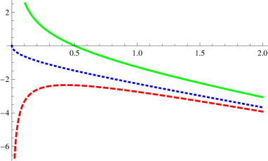
Figure 1: Cold EOS: Plots of (from below) $y_{\rm min}$ (lower boundary of the domain of the similarity solution, red, dashed), $y_{s}$ (shock location, blue, dashed) and $y_{c}$ (sonic point, green, solid) against the polytropic index $n$.

Figure 2: Cold EOS: Plot of $\bar{c}(y)$ against $y$ over the range $y_{s}\leq y\leq 10$, for $n=1$. This plot gives the instantaneous profile of the sound speed, compare Eqs. (47) and (49).

$\Gamma$	$\beta$	$\gamma$	$A$	$y_{s}$	$y_{c}$	$\tilde{c}(\infty)$
1.1	1.45455	0.3125	1.70076	-14.276	1.70076	0.556382
1.2	1.41667	0.294118	1.68007	-7.45382	1.68007	0.712463
1.3	1.38462	0.277778	1.66785	-5.08952	1.66785	0.821717
4/3	11/8	3/11	1.66534	-4.60059	1.66534	0.85234
1.4	1.35714	0.263158	1.66236	-3.84899	1.66236	0.907535
1.5	1.33333	0.25	1.66223	-3.06428	1.66223	0.978987
1.6	1.3125	0.238095	1.66638	-2.51179	1.66638	1.04075
5/3	13/10	3/13	1.67109	-2.22244	1.67109	1.07795
1.7	1.29412	0.227273	1.67394	-2.09497	1.67394	1.09559
1.8	1.27778	0.217391	1.68424	-1.76503	1.68424	1.14528
1.9	1.26316	0.208333	1.69676	-1.49452	1.69676	1.19101
2	5/4	1/5	1.71105	-1.26671	1.71105	1.23363

Table 1: Cold EOS: Table of approximate numerical values (the closed form expressions are given in the text) of $\beta$, $\gamma$, $A$, $y_{s}$, $y_{c}$ and $\tilde{c}(\infty)$ against the polytropic index $\Gamma$.

4.3 Evolution after the shock has reached the surface

The data (64) at $t=0$ are smooth, and their evolution to $t>0$ remains smooth. We were able to neglect gravity in the approach of the shock to the surface, but we must restore it in the subsequent smooth motion which occurs on a much longer timescale. This can be done exactly by going to a freely falling frame by replacing $u$ and $\xi$ with

$$\zeta \equiv x+v_{*}t-{1\over 2}gt^{2},$$ (65)

$$w \equiv v-v_{*}+gt.$$ (66)

The equations become

$$\left[\partial_{t}+(w\pm c)\partial_{\zeta}\right](w\pm 2nc)=0.$$ (67)

Clearly $w+2nc=0$ at $t=0$ and hence for $t>0$, and so the solution for $t>0$ is a simple wave characterised by

$$c_{t}-(2n+1)cc_{\zeta}=0.$$ (68)

The method of characteristics gives $c(\zeta,t)$ implicitly as

$$c=f\left[\zeta+(2n+1)ct\right],$$ (69)

where $f(x)=c(x,0)$ given in (64).

5 The solution behind the shock with the hot EOS

5.1 Matching conditions at the shock

Our numerical experiments show that the fluid velocity $v_{s}$ behind the shock does not remain constant but blows up as the shock approaches the surface. This implies that once again we are in the regime $\lambda\to 0$. From (24) with (33) we obtain

$$\sigma\simeq{\Gamma+1\over 2}v_{s}.$$ (70)

With (10), (35) gives us

$$c_{s}\simeq\sqrt{\Gamma\over 2n}v_{s}.$$ (71)

We need a third matching condition for the density. From (33), we have

$$\rho_{s}\simeq{\Gamma+1\over\Gamma-1}\rho_{0}.$$ (72)

Here the equilibrium density in front of the shock $\rho_{0}$ is given by Eq. (19).

5.2 Similarity solution

The similarity ansatz for the velocity and sound speed is similar to (47-49), namely

$$c(x,t) = {x\over t}\hat{c}(y),$$ (73)

$$v(x,t) = {x\over t}\hat{u}(y),$$ (74)

$$\rho(x,t) = C_{\rho}(-x)^{n_{*}}\tilde{\rho}(y),$$ (75)

where

$$y\equiv C_{y}(-x)(-t)^{-\beta},$$ (76)

where $C_{y}$ is a parameter (of dimension $L^{-1}T^{\beta}$) that survives from the initial data into the self-similar regime.

The relevant similarity solution begins at $y=\infty$ (corresponding to $x=-\infty$ at constant $t<0$), goes through a regular sonic point $y=y_{c}$, and ends at the shock at $y=y_{s}$. As the similarity equations are autonomous in $\eta=\ln y$, we can assume that the sonic point is at $y=1$.

We expand the solution through the regular sonic point as $\hat{u}=\hat{u}_{0}+\hat{u}_{1}\eta+O(\eta^{2})$ and $\hat{c}=\hat{c}_{0}+\hat{c}_{1}\eta+O(\eta^{2})$. For given $n_{*}$, $\beta$ and $n$, we obtain a unique value of $(\hat{u}_{0},\hat{c}_{0})$, but two values of $(\hat{u}_{1},\hat{c}_{1})$. These correspond to two smooth solution curves going through the same regular sonic point. The correct solution is easily identified by plotting.

With the shock at $\eta=\eta_{s}$, the matching conditions at the shock give

$$\hat{u}(\eta_{s}) = {2\beta\over\Gamma+1},$$ (77)

$$\hat{c}(\eta_{s}) = \sqrt{\Gamma\over 2n}\hat{u}(\eta_{s}),$$ (78)

$$\tilde{\rho}(\eta_{s}) = {\Gamma+1\over\Gamma-1}.$$ (79)

The requirement that for given $n_{*}$ and $n$ the solution curve $(\hat{u}(\eta),\hat{c}(\eta))$ goes smoothly through the sonic point and ends at the shock then determines $\beta$ and $\eta_{s}<0$ through a boundary value problem.

We solve this boundary value problem numerically by shooting from the sonic point, or rather from a small negative value of $\eta$ reached by the power-law expansion around $\eta=0$, to a trial value of $\eta_{s}$, using a trial value of $\beta$. An accurate first guess for $\eta_{s}$ and $\beta$ is obtained by approximating the solution curve from the sonic point to the shock as a linear function of $\eta$ using $\hat{u}_{1}$ and $\hat{c}_{1}$.

As in the cold case, we can write

$$c(x,t) = C_{y}^{-1}(-t)^{\beta-1}\bar{c}(y)$$ (80)

$$= C_{y}^{-{1\over\beta}}(-x)^{\gamma}\tilde{c}(y),$$ (81)

and similarly for $u(x,t)$. The limits $\tilde{c}(\infty)$ and $\tilde{u}(\infty)$ exist and are tabulated in Table 4. In contrast to the cold case, $\gamma<0$, and so $c$ and $v$ behind the shock diverge as $x\to 0_{-}$. Similarly, the instantaneous values of $c$ and $v$ just behind the shock diverge because $\beta-1<0$. In physical terms this can be thought of as a whiplash effect, where a finite amount of kinetic and internal energy is injected into ever less mass.

We can write the instantaneous density profile at $t<0$ as

$$\rho(x,t)=C_{\rho}C_{y}^{-{n_{*}}}(-t)^{n_{*}\beta}\bar{\rho}(y),\quad\bar{\rho}(y)\equiv y^{n_{*}}\tilde{\rho}(y).$$ (82)

Finally, the limit $\tilde{\rho}(\infty)$ exists and is tabulated below. Therefore the density immediately behind the shock, and the density everywhere as $t\to 0_{-}$ remain finite, as one would expect from the fact that the shock conditions show a finite compression ratio. The density profile at $t=0$ is just the one in the rest state multiplied by $\tilde{\rho}(\infty)$. This constant can be found explicitly in terms of other known constants by evaluating the integral (124) of the similarity equations at $y=y_{s}$ and as $y\to\infty$.

As a test of our calculation, Table 2 reproduces Table 1 of [Sakurai(1960)]. Focussing then on the case of an isentropic rest state, Table 4 gives key parameters of the similarity solutions for selected values of $\Gamma$.

$\Gamma\backslash n_{*}$	2	1	1/2
5/3	0.435628	0.22336	0.1141
7/5	0.3934	0.202151	0.103519
6/5	0.330985	0.170418	0.0874924

Table 2: Nonrelativistic hot EOS: Recreation of Table 1 of [Sakurai(1960)]: $1/\beta$ tabulated against $\Gamma$ (down) and $n_{*}$ (right).

$n\backslash n_{*}$	3	3/2	1
3	0.642161
3/2	0.608205	0.751791
1	0.592366	0.739586	0.807808

Table 3: Nonrelativistic hot EOS: Table of $\beta$ against $n$ and $n_{*}$. We only consider stable stratifications where $n_{*}\geq n$.

$\Gamma$	$\beta$	$\eta_{s}$	$\tilde{u}(\infty)$	$\tilde{c}(\infty)$	$\tilde{\rho}(\infty)$
1.1	0.436716	-0.0211101	0.127454	0.0190103	765.341
1.2	0.555056	-0.0468527	0.303072	0.0664771	2.01223
1.3	0.624385	-0.0722611	0.356576	0.101789	1.11067
4/3	0.642089	-0.0802736	0.368456	0.113245	0.994484
1.4	0.672222	-0.0954616	0.385789	0.135492	0.864565
1.5	0.707991	-0.116087	0.400758	0.167296	0.808397
1.6	0.736085	-0.134239	0.410263	0.198712	0.743478
5/3	0.751778	-0.14509	0.413301	0.218764	0.363108
1.7	0.758898	-0.150172	0.414418	0.228711	0.673344
1.8	0.777879	-0.164173	0.414795	0.257156	0.655824
1.9	0.793966	-0.176514	0.412426	0.283948	0.63714
2	0.807803	-0.187436	0.408344	0.309271	0.62677

Table 4: Nonrelativistic hot EOS: Table of the parameters $\beta$, $\eta_{s}$ and asymptotic values at $y=\infty$ of $\tilde{u}$, $\tilde{c}$ and $\tilde{\rho}$, against the polytropic index $n$, for the isentropic rest state case $n_{*}=n$. $\Gamma>2$ is not considered because the sound speed at ultrarelativistic temperatures is greater than the speed of light. $\Gamma=1$ is unphysical because the speed of sound is zero. We also have difficulty reaching $\Gamma=1$ when numerically solving the boundary value problem for the similarity solution.

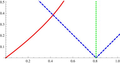
Figure 3: Nonrelativistic hot EOS: Plot of the similarity solution with $n=n_{*}=1$ in the $\hat{u}\hat{c}$ plane, illustrating the dynamical systems ideas discussed in Sec. 5.2. $\hat{u}$ is right, and $\hat{c}$ is up. The vertical straight line is the flow line and the diagonal straight line are the sonic lines (see Apppendix C). The endpoint at $\hat{u}=\hat{c}=0$ corresponds to $y=\infty$, while the other endpoint corresponds to the shock $y=y_{s}$, with the sonic point at $y_{c}=1$ by construction.

Figure 4: Nonrelativistic hot EOS: Plots of (from above) $\bar{u}(y)$ (blue, dashed), $\bar{c}(y)$ (green, dotted) and $\bar{\rho}/20$ (red, solid) for the similarity solution with $n=n_{*}=1$ for the range $y_{s}<y<e^{1}$. The sonic point is at $y_{c}=1$ by definition. These curves give the instantaneous profiles of $u$, $c$ and $\rho$ against $x$ at finite $t<0$, compare Eqs. (76), (80) (and similarly for $\bar{u}$) and (82).

5.3 New hydrostatic equilibrium after the shock

Consider now an arbitrary instantaneous state in which density and internal energy follow approximate power laws,

$$\rho \sim x^{a},$$ (83)

$$c_{s}^{2}\sim T\sim e \sim x^{b}.$$ (84)

Note that at $t=0$ in the shock heating process we have discussed, $b=2\gamma$ and $a=n_{*}$. By contrast, Eq. (21) tells us that in hydrostatic equilibrium $b=1$.

From (83) and (84) we have

$$K\sim x^{b-{a\over n}}.$$ (85)

We define the total mass per area (measured from the surface inwards) as

$$m\equiv\int_{x}^{0}\rho\,dx\sim x^{a+1}$$ (86)

and hence

$$K\sim m^{b-{a\over n}\over a+1}.$$ (87)

Let us now assume that the fluid reaches a new hydrostatic equilibrium starting from the state (83,84). This new equilibrium has a density distribution with power $\bar{a}$ and by definition has $\bar{b}=1$. If heat conduction, shock heating and other entropy-generating processes can be neglected in the approach to equilibrium, and if the fluid motion remains plane (spherically) symmetric, then the function $K=K(m)$ is unchanged, because $m$ is a Lagrangian coordinate for the plane-symmetric motion. In particular, we must have

$${b-{a\over n}\over a+1}={1-{\bar{a}\over n}\over\bar{a}+1},$$ (88)

which solves to

$$\bar{a}={(n+1)a+n(1-b)\over 1+bn}.$$ (89)

6 Numerical experiments

6.1 Numerical method

To confirm the validity of the similarity solutions presented here, we have done extensive numerical simulation using a high-resolution finite volume method designed to accurately capture shock waves. We use the open-source Clawpack software of [LeVeque et al.(2010)]. The codes used to produce the figures in this section are available at [Gundlach & LeVeque(2010)] along with more figures and animations of the results over time.

This software requires a “Riemann solver” as the basic building block. For a homogeneous conservation law with no source term, the Riemann solver takes cell averages in two neighboring grid cells and determines a set of waves propagating away from the cell interface in the solution to the Riemann problem (the conservation law with piecewise constant intial data). A simple update of the cell averages based on the distance these waves propagate into the cells gives the classic Godunov method, a robust but only first-order accurate numerical method. Second order correction terms can be defined in terms of these waves and then limiters are applied to these terms in order to avoid non-physical oscillations in the solution. This is crucial near discontinuities for problems involving shock waves, particularly when near a vacuum state as in the present problem. Complete details of the algorithms implemented in Clawpack can be found in [LeVeque(2002)], [LeVeque(1997)]. Several other books also discuss shock-capturing finite volume methods based on Riemann solvers, such as [Toro(1997)] and [Trangenstein(2009)]. The development of high-resolution shock-capturing methods has a long history, and many references can be found in the books cited above.

The discussion here will focus on several modifications that have been made to the standard software in order to handle the demands of the present problem. We use the f-wave formulation of the the wave-propagation algorithm originally proposed in [Bale et al.(2002)] in order to obtain a “well-balanced” method that preserves the steady state equilibrium solution in the stationary atmosphere ahead of the shock wave, following the approach in [LeVeque(2010)]. Maintaining this steady state requires that the pressure gradient in (2) balances the source term $-g\rho$. In the f-wave formulation, the flux difference between adjacent cells is modified by the source terms and the Riemann solver applied to this modified flux difference to obtain f-waves that are used in place of the classic waves of the Riemann solution. If the source terms are appropriately discretized at each interface, the method will be well balanced in the sense that initial data that are in equilibrium will lead to zero-strength f-waves in each Riemann solution and hence no modification to the solution. Moreover, small perturbations to an equilibrium solution will result in small amplitude f-waves. The limiters are applied to these f-waves and much more accurate solutions can be obtained for certain quasi-steady problems with this approach than with techniques such as fractional step methods (in which one alternates between solving the homogeneous conservation law and applying the source terms). Discretization of the source term $-g\rho$ requires defining an appropriate average of the densities from the two cells bordering each interface and we use the approach suggested in [LeVeque(2010)] to achieve a well-balanced method for the atmosphere at rest.

The Riemann solver for the f-wave method must then take the flux difference between two cells, as modified by the source term, and split this vector into waves propagating to the left and right that are used to update neighboring cell averages. This is typically done by splitting the vector into eigenvectors of some approximate Jacobian matrix such as the one produced by a Roe average of the neighboring states. However, near vacuum state the standard approach can lead to negative pressures or densities and a breakdown of the method. We use a variant of the Siliciu relaxation solver described in Sections 2.4.4–6 of [Bouchut(2004)], which is related to the HLLE solver. This solver has been modified to work with the f-wave formulation in recent work with [Murphy(2009)].

To see the self-similar structure that eventually develops, we need to zoom in by many orders of magnitude in the vicinity of $x=0$ at the times just before the shock reaches the origin. For general initial data specified at some time $t_{0}$ it is impossible to determine a priori the exact final time $t_{f}$ when the shock will reach $x=0$, and it varies depending on the mesh spacing and the choice of computational parameters such as the limiter used to maintain stability. For the computations presented here we have used the monotonized centered (MC) limiter (see [LeVeque(2002)]), which is generally a good limiter for nonlinear systems that gives sharper results than the minmod limiter but greater stability than superbee, for example. We have also tried minmod and obtain similar results. Note that the parameter $t$ used elsewhere in the paper for the similarity solution corresponds to $t=t_{c}-t_{f}$ where $t_{c}$ is the time variable in the computation. We start the computation with $t_{c}=0$ but reset to $t_{c}=0$ at some point as we approach the final time in order to retain more significant figures in $t$.

We compute on a domain $x_{\text{min}}\leq x\leq 0$ which is divided into $M$ finite volume cells. Initially $x_{\text{min}}=-12$, but we repeatedly cut the domain in half by halving both $x_{\text{min}}$ and $\Delta x$ in order to zoom in on the origin. In each time step we estimate the current shock location $x_{s}$ as the location of the largest change in density and we perform this regridding as soon as $x_{s}>0.1x_{\text{min}}$, i.e., when the shock is 90% of the way to the boundary. Regridding is performed by taking the solution on the right half of the domain and doubling the resolution, so that $M$ remains the same while $x_{\text{min}}$ and $\Delta x$ are halved. In each grid cell $j=M/2+1,~{}\ldots,~{}M$ we estimate a slope for each component of the solution by applying a limiter to the one-sided slopes to the left and right, and use this to construct a linear function passing through the cell average with this slope (essentially identical results are obtained with either the minmod or superbee limiters). We sample the resulting linear function at the midpoint of the left and right halves of the cell. These two values replace the values stored in cells $i$ and $i+1$, where $i=2(j-M/2)-1$. This procedure is conservative since the two new values have the same mean value as the previous single value. It is second order accurate where the solution is smooth, but it does introduce some artifacts at the shock. The new interpolated values do not lie exactly on the numerical shock Hugoniot for a propagating shock and hence small oscillations generally emerge from the shock at the regridding times that propagate into the flow behind the shock. These are quite minor and do not hamper our ability to see the expected self-similar behavior.

The time step $\Delta t$ is chosen automatically by the Clawpack software, based on a user-supplied target Courant number, which we take to be 0.8. The Courant number is computed in each time step as

$${\text{\bf}CFL}=\frac{\Delta t}{\Delta x}\max_{i,p}|s_{i}^{p}|$$ (90)

where $s_{i}^{p}$ is the wave speed of the $p$th wave for the Riemann problem between cells $i-1$ and $i$. The time step $\Delta t$ for the next step is chosen by setting ${\text{\bf}CFL}$ in (90) to the target Courant number and solving for $\Delta t$. (The actual Courant number in the next step may differ from the target since the nonlinear wave speeds $s_{i}^{p}$ are recomputed in each step. If the actual Courant number is larger than the stability limit of 1 then the step is re-taken with a smaller $\Delta t$, which at this point can be calculated to hit the target Courant number exactly since the waves speeds are now known.) Using this mechanism, the time step automatically scales with $\Delta x$ as the computational domain is subdivided. We output results every $N_{\text{out}}$ time steps (some fixed number depending on $M$) to obtain snapshots of the solution as it gets further into the asymptotic regime. The space-time numerical grids used resemble a set of nested boxes all sharing the top right corner at $x=0,~{}t_{c}=t_{f}$. Note that with this strategy the shock never reaches $x=0$ and we typically halt the computation when $x_{\text{min}}\approx 10^{-10}$ (after about 35 domain halvings).

From the final frames of the solution we can estimate $t_{f}$, the time when the shock would hit $x=0$. As mentioned above, to obtain enough significant figures in $t_{f}-t_{c}$ we reset $t_{c}$ to 0 at some point in the computation, typically when $x_{\text{min}}\approx-10^{-6}$.

For boundary conditions at $x=x_{\text{min}}$ we use the zero-order extrapolation conditions that are often used in Clawpack to avoid non-physical reflections at computational boundaries. The values in the first interior grid cell are simply copied to ghost cells adjacent to the cell before each time step as described in Chapter 5 of [LeVeque(2002)]. This is obviously unphysical in that it does not represent the overall solution that we have cut off. However, this has no influence on the portion of the solution we are interested in. After regridding, the shock has been shifted from $x\approx 0.1x_{\text{min}}$ to $x\approx 0.2x_{\text{min}}$ after $x_{\text{min}}$ is halved. Using an explicit method with Courant number less than 1, information can propagate no more than 1 grid cell per time step. Hence in the time between regriddings any effect of boundary conditions at $x=x_{\text{min}}$ can contaminate at most 10% of the cells before the next regridding takes place, at which point we throw away the left half of the cells. So these boundary conditions can never affect the solution near the shock wave.

The boundary condition imposed at $x=0$ is immaterial for this work since we never allow the shock to reach the boundary. We need only insure that the equilibrium solution is not disturbed adjacent to the boundary. We use a well-balanced method as described above that maintains the steady state between regridding times. Unfortunately, this is disturbed by regridding since reconstructing and sampling a piecewise linear function as described above gives new cell values that are not in exact equilibrium. So in the undisturbed region ahead of the shock we reset the solution by evaluting the exact form of the known equilibrium solution on the new finer grid each time we regrid.

6.2 Cold equation of state

For the cold EOS with $n=1$, the equilibrium solution has $\rho(x)=-x$, $v(x)=0$, and $c(x)=\sqrt{-x}$. For numerical experiments we perturbed this with strong generic displacements in density and momentum centered about different points, namely

$$\rho(x,0) = -x+10\exp\left(-((x+11)/0.3)^{2}\right),$$ (91)

$$(\rho v)(x,0) = 30\exp\left(-((x+10)/0.3)^{2}\right),$$ (92)

on $-12\leq x\leq 0$. The late-time behaviour is independent of these initial data except for the fitting of the free parameters $v_{*}$ and $t_{c}$, thus showing that the similarity solution is universal. Figures 5 through 7 show results for this case.

For this case, $M=4800$ grid cells were used and we took 40000 time steps, at which point the shock was within distance $1\times 10^{-14}$ of the origin. This required less than 3 minutes of CPU time on a MacBook Pro using a single 2.2GHz processor.

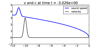
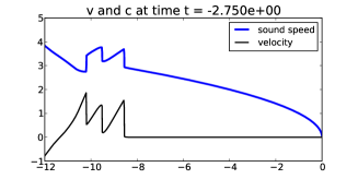
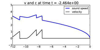
Figure 5: Numerical solution for the cold EOS $n=1.0$, showing the fluid velocity and sound speed after 0, 800, 1600, and 8000 time steps on a grid with $M=4800$ grid cells. The generic Gaussian initial data breaks up into left-going and right-going waves. The times listed here and in later figures are $t_{c}-t_{f}$ as discussed in the text, corresponding to $t$ of the similarity solution.

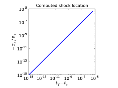
Figure 6: Computed shock location for the cold EOS with $n=1$, illustrating that the shock has constant speed $v_{*}$ as $t_{c}\to t_{f}$ over many decades. Results of more than 21000 time steps are plotted (with $M=4800$) on a log-log scale.

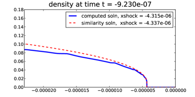
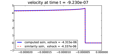
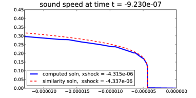
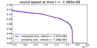
Figure 7: Cold equation of state with $n=1$. The density (top), velocity (middle), and sound speed (bottom) at two different times. The left column shows the solution after 20000 time steps and the right column shows the solution after 24000 time steps. In all cases the solid blue curve is the computed solution with $M=4800$ grid cells and the red dashed curve is the similarity solution. For animations, see [Gundlach & LeVeque(2010)].

A wave travelling right has sharpened into a double N-wave by the time its leading edge has reached $x=-8.5$. By the time the leading edge has reached $x=-3.4$, the leading N-wave has been caught up by and merged with the second N-wave, and the wave going left has steepened into an N-wave and completely left the grid.

The expected similarity solution is obtained by solving Eq. (56), multiplied by $y$, numerically for $\bar{c}(y)\equiv y\hat{c}(y)$. The parameters $v_{*}$ and $t_{f}$ (the final time, when the shock arrives at the surface) must be fit from the computed solution. For late times in the computation, the shock appears to propagate at nearly constant velocity and fitting a linear function to the observed shock location gives an estimate for $t_{f}$. The constant velocity should be $v_{*}$, but we have found that a more accurate estimate of $v_{*}$ is obtained by examining the Riemann invariant $v+2nc=v_{*}={\rm const}$, which is very nearly constant behind the shock in the computed solution.

As $x_{s}\to 0$, the instantaneous profiles of $c$ and $v$ in the numerical solution behind the shock begin to resemble the similarity solution first in shape and in the shock location while an overall factor in $c$ and $v$ agrees only later. By the time the shock is at $x_{s}\sim 10^{-3}$, there is agreement within a factor of 2. The agreement is convincing by the time the shock has reached $x_{s}\sim 10^{-6}$. This is a strong indication that the similarity solution is an attractor, at sufficiently small $x_{s}$ and $t_{c}-t_{f}$. The relevant dimensionless number here is that $x_{s}$ is about $10^{-6}$ times its value when a shock first formed from generic initial data. As $x_{s}\to 0$ as $t_{c}-t_{f}\to 0_{-}$, the agreement is very good at late times, as illustrated in Figure 6.

Figure 7 shows the results after 20000 and 24000 time steps, illustrating close agreement with the similarity solution. At later times the agreement is not so good though convergence tests show that at any fixed time there is increasingly good agreement as the grid is refined.

6.3 Hot equation of state

Figures 8 through 10 show results for three hot EOS cases: $n=n_{*}=1,~{}n=n_{*}=1.5$, and $n=1,~{}n_{*}=1.5$. The initial behaviour of the shocks is qualitatively similar to the cold EOS case. The late-time behaviour approaches the similarity solution and is again independent of the initial data except for the fitting of the free parameters $C_{y}$ and $t_{c}$. Note the very different scaling of the axes in each case.

The hot EOS case is easier to compute than cold EOS case and all of these results are shown on grids with $M=1200$ cells. Finer grids give even closer agreement. With $M=4800$ the computed solution is indistinguishable from the similarity solutions to plotting accuracy. Moreover, the solutions continue to match well out to $x_{s}\sim 10^{-15}$, after starting to agree with the similarity solution very well at $t\sim 10^{-3}$, when $x_{s}\sim 0.01$.

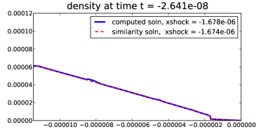
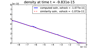
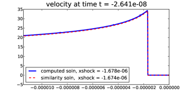
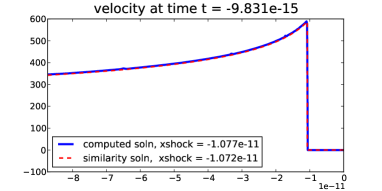
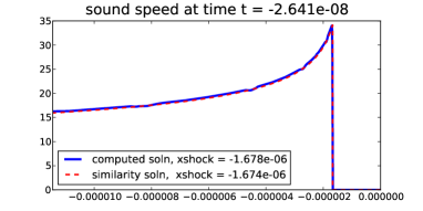
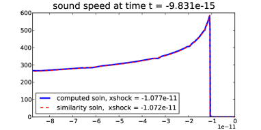
Figure 8: Hot equation of state with $n=n_{*}=1$. The density (top), velocity (middle), and sound speed (bottom) at two different times. The left column shows the solution after 6000 time steps and the right column shows the solution after 10000 time steps. In all cases the solid blue curve is the computed solution with $M=1200$ grid cells and the red dashed curve is the similarity solution. For animations, see [Gundlach & LeVeque(2010)].

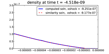
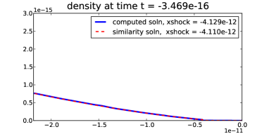
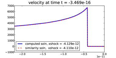
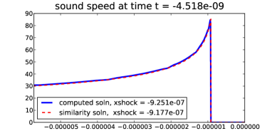
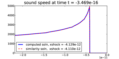
Figure 9: Hot equation of state with $n=n_{*}=1.5$. The density (top), velocity (middle), and sound speed (bottom) at two different times. The left column shows the solution after 6000 time steps and the right column shows the solution after 10000 time steps. In all cases the solid blue curve is the computed solution with $M=1200$ grid cells and the red dashed curve is the similarity solution. For animations, see [Gundlach & LeVeque(2010)].

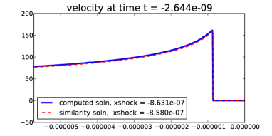
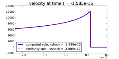
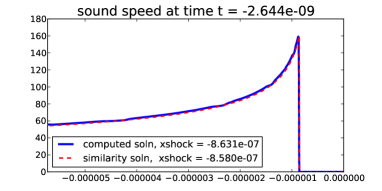
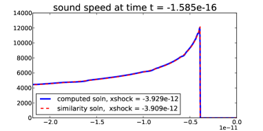
Figure 10: Hot equation of state with $n=1.0,~{}~{}n_{*}=1.5$. The density (top), velocity (middle), and sound speed (bottom) at two different times. The left column shows the solution after 6000 time steps and the right column shows the solution after 10000 time steps. In all cases the solid blue curve is the computed solution with $M=1200$ grid cells and the red dashed curve is the similarity solution. For animations, see [Gundlach & LeVeque(2010)].

7 Conclusions

We have constructed similarity solutions that describe a shock approaching the surface of a star from the interior, in the limit where the shock is very close to the surface and can be approximated as planar. We have shown by numerical simulation in the planar approximation that generic initial data approach the similarity solution as a universal endstate as the shock approaches the surface.

The behaviour is very different for cold and hot equations of state. In the cold EOS, the fluid behind the shock moves to leading order as a single body, with the matter still in front of the shock getting stuck on like insects to the front of a car, and dynamically insignificant. The density directly behind the shock becomes ever larger than that in front, and the velocity directly behind the shock approaches a constant.

With the hot equation of state, shock heating becomes essential, and this indicates that the cold EOS approximation is completely wrong for shocks near the surface. The ratio of densities in front and behind the shock approaches a constant. The fluid velocity and sound speed behind the shock diverge, which means that eventually the motion has to be treated relativistically. There would then be a (non-self-similar) transition to a new, ultra-relativistic similarity solution, where one also has to assume that $P=\rho e/3$. This ultra-relativistic solution has been investigated by [Nakayama & Shigeyama(2005)], but it would depend on the physical circumstances if it becomes relevant before the perfect fluid approximation breaks down (and has to be replaced, for example, by kinetic theory) at the surface of the star.

We hope that our solutions provide at least rough approximations to shock formation near a stellar surface in some circumstances. They are also good testbeds for codes capable of dealing with stellar surfaces. Our simulations are based on the Clawpack software but required some modification to standard methods in order to compute into the similarity regime. In particular, we have used a well-balanced approach that maintains the hydrostatic equilibrium ahead of the shock to machine precision and a remeshing procedure to obtain well resolved solutions down to $x_{s}\sim 10^{-15}$.

In an appendix, we have given a self-contained derivation of the similarity solution. We stress how similarity solutions for the cold equation of state can be identified with isentropic similarity solutions for the hot equation of state, and under what circumstances any conservation law in the original fluid equations gives rise to an integral of the motion in the ordinary differential equations resulting from a similarity ansatz.

Appendix A General notes on similarity solutions

A.1 Transport laws

Consider a transport law of the form

$$\varphi_{t}+v\varphi_{x}=0,$$ (93)

where $v$ is a velocity, and the dimension of $\varphi$ is undetermined. Without loss of generality, we can write any power-law similarity ansatz as

$$\varphi = x^{\alpha}\tilde{\varphi}(y),$$ (94)

$$v = x^{\gamma}\tilde{v}(y),$$ (95)

where

$$y\equiv xt^{-\beta}.$$ (96)

(Any more general ansatz is related to this by redefining $y$, $\tilde{v}$ and $\tilde{\varphi}$.) In order to obtain an ODE in $y$ alone, we require

$$\gamma=1-{1\over\beta}\Leftrightarrow\beta={1\over 1-\gamma}.$$ (97)

The resulting ODE can be simplified by defining

$$\hat{v}(y)\equiv y^{-{1\over\beta}}\tilde{v}(y),$$ (98)

and becomes

$$\left(\hat{v}-\beta\right)y\tilde{\varphi}^{\prime}+\alpha\hat{v}\tilde{\varphi}=0.$$ (99)

This redefinition is equivalent to defining

$$v={x\over t}\hat{v}(y).$$ (100)

This no longer contains $\gamma$, and makes $\hat{v}$ dimensionless.

If, in particular, $\alpha=\gamma$, and we define $\tilde{\varphi}(y)\equiv y^{1/\beta}\hat{\varphi}(y)$, the transport law becomes

$$\left(\hat{v}-\beta\right)y\hat{\varphi}^{\prime}+(\hat{v}-1)\hat{\varphi}=0.$$ (101)

A.2 Conservation laws and integrals

Consider the conservation law

$$\varphi_{t}+F_{x}=0.$$ (102)

Without loss of generality, the most general power law similarity ansatz that results in an ODE is

$$\varphi = x^{\alpha}\tilde{\varphi}(y),$$ (103)

$$F = x^{\alpha+1}t^{-1}\tilde{F}(y),$$ (104)

and this ODE is

$$-\beta\tilde{\varphi}^{\prime}+\tilde{F}^{\prime}+{\alpha+1\over y}\tilde{F}=0.$$ (105)

If and only if $\alpha=-1$, this admits an integral of the form

$$\tilde{F}-\beta\tilde{\varphi}=\rm const.$$ (106)

In particular, if $F=v\varphi$, so that we have

$$\varphi_{t}+(v\varphi)_{x}=0,$$ (107)

and making the consistent ansatz (100), we have

$$\left(\hat{v}-\beta\right)\tilde{\varphi}=\rm const.$$ (108)

Usually, however, we cannot arrange for $\alpha=-1$.

By contrast, if we have a conserved mass density $\rho$, then any quantity $K$ that is constant along fluid world lines gives rise to an integral of the ODEs in the self-similarity ansatz. From

$$K_{t}+vK_{x} = 0,$$ (109)

$$\rho_{t}+(v\rho)_{x} = 0,$$ (110)

we get

$$(\rho K^{p})_{t}+(v\rho K^{p})_{x}=0,$$ (111)

for any $p$. Assuming

$$\rho = x^{\alpha}\tilde{\rho}(y),$$ (112)

$$K = x^{\nu}\tilde{K}(y),$$ (113)

and (100), we can now choose $p=-(\alpha+1)/\nu$, and obtain

$$\left(\hat{v}-\beta\right)\tilde{\rho}\tilde{K}^{p}=\rm const.$$ (114)

without any restriction on $\nu$.

Appendix B Cold polytropic gas dynamics

B.1 Similarity ansatz

In gas dynamics $u$ and $c$ both scale as velocities. Therefore, with the ansatz

$$u = {\xi\over t}\hat{u}(y),$$ (115)

$$c = {\xi\over t}\hat{c}(y),$$ (116)

the equations (44) with $g=0$, using (101), become

$$\left(\hat{u}\pm\hat{c}-1\right)\left(\hat{u}\pm 2n\hat{c}\right)+\left(\hat{u}\pm\hat{c}-\beta\right)y\left(\hat{u}\pm 2n\hat{c}\right)^{\prime}=0.$$ (117)

These equations become automous in the independent variable $\eta=\ln y$, thus defining a dynamical system in the $\hat{u}\hat{c}$-plane. The direction field is reflection-symmetric about the line $\hat{c}=0$, and trajectories cannot cross this line, so that we can assume $\hat{c}>0$.

We note in passing that a self-similar solution can be obtained also for $g\neq 0$ if we set $\beta=2$. The dimensionless self-similarity variable is then $y=x/(gt^{2})$, from dimensional analysis (self-similarity of the first kind).

B.2 Dynamical system analysis

The general solution for $\beta=1$ is the trivial one $u=u_{0}$, $c=c_{0}$.

For $\beta\neq 1$, the lines $\hat{c}=\pm(\hat{u}-\beta)$ define sonic points, where the lines of constant $y$ are tangential to one of the two fluid characteristics in the $xt$-plane. The abstract dynamical system is regular there, with $d\hat{c}/d\hat{u}=\mp 1/(2n)$, but the ODEs in $y$ or $\eta$ are in general singular there, with $d\epsilon/d\eta\sim 1/\epsilon$, where $\epsilon$ is the distance to the line, and so solution curves end there with $\epsilon\sim\sqrt{\eta_{0}-\eta}$.

However, on each line of sonic points, there is one regular sonic point given by $\hat{c}=\pm\hat{u}/(2n)$, where $d\epsilon/d\eta$ is finite (because both its numerator and denominator vanish). They are

$$\hat{c}=\pm{\beta\over 2n-1},\qquad\hat{u}={2n\beta\over 2n-1}.$$ (118)

Precisely one of these is in the physical region $\hat{c}>0$, depending on the sign of $\beta$ and $2n-1$.

There are two smooth solutions through each of these points, with slopes

$${d\hat{c}\over d\hat{u}}=\mp{1\over 2n},\mp{(\beta-1)(4n^{2}+1)+4n\over 4n\left[1+2n(\beta-1)\right]}.$$ (119)

A further power-law expansion shows that for the first of these solutions $\hat{c}=\pm 2n\hat{u}$ to all orders. One of the two ODEs (117) is then identically satisfied, and the remaining one becomes separable when written in $\hat{c}$ alone and is independent of the sign $\pm$ above. An implicit solution in closed form is given in (56-57) above.

Appendix C Hot polytropic gas dynamics

C.1 Similarity ansatz

A useful form of the general power-law similarity ansatz is

$$\rho = x^{n_{*}}\tilde{\rho}(y),$$ (120)

$$u = {x\over t}\hat{u}(y),$$ (121)

$$c = {x\over t}\hat{c}(y).$$ (122)

In the variable $\eta=\ln y$ the the resulting ODEs are autonomous. Furthermore, their right-hand sides are rational functions of only $\hat{u}$, $\hat{c}$ and the parameters ${n_{*}}$, $\beta$ and $n$. This means that we have a dynamical system in the $\hat{u}\hat{c}$-plane, with $\ln\rho$ slaved to $\hat{u}$ and $\hat{c}$. Again we assume that $\hat{c}>0$.

C.2 Integral of the motion

The reason that $\tilde{\rho}$ does not appear on the right-hand sides is that $K$ is constant on fluid worldlines, and hence that an integral of the motion exists. We have

$$\Gamma K = c^{2}\rho^{-{1\over n}}=x^{2-{{n_{*}}\over n}}t^{-2}\hat{c}^{2}\tilde{\rho}^{-{1\over n}}$$ (123)

$$= x^{2-{{n_{*}}\over n}-{2\over\beta}}y^{2\over\beta}\hat{c}^{2}\tilde{\rho}^{-{1\over n}}$$

From our discussion in Sec. A.2 we now have the integral

$$\left(\hat{u}-\beta\right)y^{2p\over\beta}\hat{c}^{2p}\tilde{\rho}^{1-{p\over n}}=\rm const.,$$ (124)

where

$$p\equiv-{{n_{*}}+1\over q},\qquad q\equiv 2-{{n_{*}}\over n}-{2\over\beta}.$$ (125)

C.3 Isentropic limit

To compare the ODEs for $\hat{u}$ and $\hat{c}$ with their counterparts for the cold EOS, we can write them in the form

$$\left(\hat{u}\pm\hat{c}-1\right)\left(\hat{u}\pm 2n\hat{c}\right)+\left(\hat{u}\pm\hat{c}-\beta\right)y\left(\hat{u}\pm 2n\hat{c}\right)^{\prime}$$ (126)

$$= -{n\beta q\over\Gamma}{\hat{c}^{2}\over\hat{u}-\beta}.$$

The right-hand side in this equation corresponds to the right-hand side in Eq. (13).

The cold similarity equations (13) are obtained as the case $q=0$ of the hot EOS similarity equations (126). Conversely, the limit $q\to 0$ of the integral (124) is

$$y^{2\over\beta}\hat{c}(y)^{2}\tilde{\rho}(y)^{-{1\over n}}={\rm const}.$$ (127)

and from (123) we see that $K$ is constant. Therefore, any combination of ${n_{*}}$, $\beta$ and $n$ such that $q=0$ represents an instant of the isentropic limit of the hot EOS case, and conversely, any similarity solution with the cold EOS can be interpreted as an isentropic similarity solution with the hot EOS, with ${n_{*}}$ given by $q=0$, and $\tilde{\rho}(y)$ given by (127).

C.4 Dynamical system analysis

In general, $\hat{u}^{\prime}(\eta)$ and $\hat{c}^{\prime}(\eta)$ are singular (their denominators vanish) on the straight lines $\hat{u}-\beta=0$ and $\hat{c}=\pm(\hat{u}-\beta)$. These lines divide the half-plane $\hat{c}>0$ into four sectors.

Limits $y\to 0$ and $y\to\infty$

For $|\hat{c}|,|\hat{u}|\gg 1,|\beta|$, we have $\hat{u},\hat{c}\sim y^{-1}$ as $y\to 0$ and and for $|\hat{c}|,|\hat{u}|\ll 1,|\beta|$, we have $\hat{u},\hat{c}\sim y^{-1/\beta}$ as $y\to\infty$. The limit of $\hat{u}/\hat{c}$ is undetermined.

Flow line $\hat{u}=\beta$

The line $\hat{u}=\beta$ represents points where a fluid world line coincides with a similarity line. Let us call it the flow line. Near it, $\hat{u}-\beta\sim\eta-\eta_{0}$ and $\hat{c}\sim(\eta-\eta_{0})^{-\beta q/2\Gamma}$. So solutions end there at finite $\eta$ but in the dynamical system it is an asymptote.

Sonic lines $\hat{c}=\pm(\hat{u}-\beta)$

The two other lines represent sonic points, where a sound characteristic coincides with a similarity line of constant $y$. We shall call them the sonic lines of the dynamical system. The dynamical system is regular there, with $d\hat{c}/d\hat{u}=\mp 1/(2n)$, but the ODEs in $y$ or $\eta$ are singular there, with $d\epsilon/d\eta\sim 1/\epsilon$, where $\epsilon$ is the distance to the line, and so solution curves end there with $\epsilon\sim\sqrt{\eta_{0}-\eta}$. On each sonic line, there is also one regular sonic point where the $y$ or $\eta$ derivatives are also finite. Exactly one of these is in the physical region $\hat{c}>0$, depending on ${n_{*}}$, $\beta$ and $n$. Through each regular sonic point there are two smooth solutions.

C.5 Special case $\beta=1$

For $\beta=1$, the regular sonic points move down to $\hat{c}=0$, $\hat{u}=1$. There the solution ends because $\hat{c}$ cannot change sign.

For $\beta=1$ only, the Galileo transformation $u\to u+v_{*}$ relates different solutions of the similarity ODEs, so that any solution $(\hat{u}(y),\hat{v}(y))$ can be obtained from a reference solution $(\hat{u}_{*}(y),\hat{v}_{*}(y))$ as

$$\hat{u}(y)-1 = \left(1-{A\over y}\right)\Bigl{[}\hat{u}_{*}(y-A)-1\Bigr{]},$$ (128)

$$\hat{c}(y) = \left(1-{A\over y}\right)\hat{c}_{*}(y-A),$$ (129)

where $A$ is a real constant. Note that this transformation does not mix solutions in the four sectors, so one needs one reference solution in each sector to fill the phase plane.

References

- [Baiotti et al.(2008)] Baiotti, L., Giacomazzo, B. & Rezzolla, L. 2008 Accurate evolutions of inspiralling neutron-star binaries: prompt and delayed collapse to black hole. Phys. Rev. D 78, 084033.
- [Bale et al.(2002)] Bale, D., LeVeque, R. J., Mitran, S. & Rossmanith, J. A. 2002 A wave-propagation method for conservation laws and balance laws with spatially varying flux functions. SIAM J. Sci. Comput. 24, 955–978.
- [Barker & Whitham(1980)] Barker, J. W. & Whitham, G. B. 1980 The similarity solution for a bore on a beach. Comm. Pure Appl. Math. 33, 447–460.
- [Bauswein et al.(2010)] Bauswein, A., Janka, H.-Th. & Oechslin, R. 2010 Testing approximations of thermal effects in neutron star merger simulations. submitted to Phys. Rev. D.
- [Berger & Kohn(1988)] Berger, M. & Kohn, R. 1988 A rescaling algorithm for the numerical calculation of blowing-up solutions. Comm. Pure Appl. Math. 41, 841–863.
- [Bouchut(2004)] Bouchut, F. 2004 Nonlinear stability of finite volume methods for hyperbolic conservation laws and well-balanced schemes for sources. Boston: Birkhäuser.
- [Duez(2009)] M. D. Duez 2009 Numerical relativity confronts compact neutron star binaries: a review and status report, Class. Quantum Grav. 27, 114002.
- [Etienne et al.(2009)] Etienne, Z. B., Liu, Y. T, Shapiro, S. L. & Baumgarte, T. W. 2009 Relativistic simulations of black hole-neutron star mergers: Effects of black-hole spin. Phys. Rev. D 79, 044024.
- [Font(2008)] Font, J. A. 2008 Numerical hydrodynamics and magnetohydrodynamics in general relativity. Living Reviews in Relativity 2008-7.
-
[Gundlach & LeVeque(2010)]
Gundlach, C. & LeVeque, R. J. 2010 codes and simulations for this paper.
www.clawpack.org/links/shockvacuum10. - [Gundlach & Murphy(2010)] Gundlach, C. & Murphy, J. 2010 Tidal shock waves in binaries. in preparation.
- [Gundlach & Please(2010)] Gundlach, C. & Please, C. 2009 Generic behaviour of nonlinear sound waves near the surface of a star: smooth solutions, Phys. Rev. D 79, 067501; Erratum ibid. D 79, 089901 (2009).
- [H. B. Keller & Whitham(1959)] H. B. Keller, D. A. Levine & Whitham, G. B. 1959 Motion of a bore over a sloping beach. J. Fluid Mech. 7, 302.
- [Kiuchi et al.(2009)] Kiuchi, K., Sekiguchi, Y., Shibata, M. & Taniguchi, K. 064037 Longterm general relativistic simulation of binary neutron stars collapsing to a black hole. Phys. Rev. D 80, 064037.
- [Kyutoku et al.(2010)] Kyutoku, K., Shibata, M. & Taniguchi, K. 2010 Gravitational waves from nonspinning black hole-neutron star binaries: dependence on equations of state. accepted for publication in Phys. Rev. D.
- [LeVeque(1997)] LeVeque, R. J. 1997 Wave propagation algorithms for multi-dimensional hyperbolic systems. J. Comput. Phys. 131, 327–353.
- [LeVeque(2002)] LeVeque, R. J. 2002 Finite Volume Methods for Hyperbolic Problems. Cambridge University Press.
- [LeVeque(2010)] LeVeque, R. J. 2010 A well-balanced path-integral f-wave method for hyperbolic problems with source terms. To appear in J. Sci. Comput., www.clawpack.org/links/wbfwave10.
- [LeVeque et al.(2010)] LeVeque, R. J. et al. 2010 clawpack software. www.clawpack.org.
- [Murphy(2009)] Murphy, J. 2009 Personal communication.
- [Nakayama & Shigeyama(2005)] Nakayama, K. & Shigeyama, T. 2005 Self-similar evolution of relativistic shock waves emerging from plane-parallel atmospheres. Astrophys. J. 627, 310–318.
- [Oechslin et al.(2002)] Oechslin, R., Rosswog, S. & Thielemann, F.-K. 2002 Conformally flat smoothed particle hydrodynamics: Application to neutron star mergers. Phys. Rev. D 65, 103005.
- [Baiotti et al.(2008)] L. Baiotti, B. Giacomazzo & L. Rezzolla 2008 Accurate evolutions of inspiralling neutron-star binaries: prompt and delayed collapse to black hole, Phys. Rev. D 78, 084033.
- [Sakurai(1960)] Sakurai, A. 1960 On the problem of a shock wave arriving at the edge of a gas. Comm. Pure Appl. Math. 13, 353–370.
- [Toro(1997)] Toro, E. F. 1997 Riemann Solvers and Numerical Methods for Fluid Dynamics. Berlin, Heidelberg: Springer-Verlag.
- [Trangenstein(2009)] Trangenstein, J. 2009 Numerical Solution of Hyperbolic Partial Differential Equations. Cambridge University Press.