The ground state of binary systems with a periodic modulation of the linear coupling

Abstract

We consider a quasi-one-dimensional two-component systm, described by a pair of Nonlinear Schrödinger/Gross-Pitaevskii Equations (NLSEs/GPEs), which are coupled by the linear mixing, with local strength $\Omega$, and by the nonlinear incoherent interaction. We assume the self-repulsive nonlinearity in both components, and include effects of a harmonic trapping potential. The model may be realized in terms of periodically modulated slab waveguides in nonlinear optics, and in Bose-Einstein condensates too. Depending on the strengths of the linear and nonlinear couplings between the components, the ground states (GSs) in such binary systems may be symmetric or asymmetric. In this work, we introduce a periodic spatial modulation of the linear coupling, making $\Omega$ an odd, or even function of the coordinate. The sign flips of $\Omega(x)$ strongly modify the structure of the GS in the binary system, as the relative sign of its components tends to lock to the local sign of $\Omega$. Using a systematic numerical analysis, and an analytical approximation, we demonstrate that the GS of the trapped system contains one or several kinks (dark solitons) in one component, while the other component does not change its sign. Final results are presented in the form of maps showing the number of kinks in the GS as a function of the system’s parameters, with the odd/even modulation function giving rise to the odd/even number of the kinks. The modulation of $\Omega(x)$ also produces a strong effect on the transition between states with nearly equal and strongly unequal amplitudes of the two components.

I Introduction

Currently available experimental techniques make it possible to create two-component Bose-Einstein condensates (BEC). In the first experiments on such systems mixtures of different hyperfine atomic states were used, such as atoms of ⁸⁷Rb with different values of the total spin, $F$ trapp . Such binary BEC systems offer straightforward possibilities for the realization of novel quantum phase transitions. In particular, while the superfluids formed by ⁸⁷Rb atoms in states $\left|F=1,m_{F}=-1\right\rangle$ and $\left|F=2,m_{F}=+1\right\rangle$ are immiscible, the proximity of this system to the miscibility threshold makes it possible to create specific phase-separation patterns Rb-separation . On the other hand, the pair of $\left|F=1,m_{F}=1\right\rangle$ and $\left|F=2,m_{F}=2\right\rangle$ states form a miscible superfluid, in which the separation between the species may be induced by an external field or by a specific flow pattern Ketterle . The immiscibility-miscibility border in binary systems may be shifted by means of the Feshbach-resonance technique, which changes the strength of the nonlinear interactions using external magnetic or optical fields Feshbach .

Novel avenues in the physics of multicomponent BECs were opened with an realization of all-optical trapping and creation of spinor condensates, where the different components correspond to the different Zeeman levels of a given hyperfine manifold of spin $F$ (for reviews cf. vandruten ; lewen-annals ; Zawist ). In this case , in principle, the number of (relevant) components can be controlled (from $2$ to $2F+1$) using optical methods, and Feshbach resonances may be used to tune the desired collisional channels.

Very accurate models for the description of BEC in quantum gases are provided by the Gross-Pitaevskii equation (GPE), or systems of coupled GPEs, in the case of the binary system GPE . With the help of these equations, ground states (GSs) of the binary systems ground and excitations on top of them Mason have been studied in detail. A well-known pattern created by the immiscibility in the binary BEC is the domain wall between spatial regions occupied by the different species domain , which may also be accurately described by means of coupled GPEs Tripp .

An additional physically interesting ingredient of the binary-condensate settings is a possibility to induce the interconversion in the mixture of two hyperfine, or Zeeman states of the same atom by an electromagnetic spin-flipping field BBS , or a two-photon Raman transition (cf. vandruten ). In terms of the coupled GPEs, the interconversion is accounted for by linear-coupling terms. Diverse effects have been predicted in such models, including Josephson oscillations between the states Josephson , domain walls DWs , “co-breathing” oscillation modes in the mixture breathing , nontopological vortices vortex , a linear-mixing-induced shift of the miscibility-immiscibility transition Merhasin , spontaneous symmetry breaking in two-component gap solitons SKA , etc.

Similar models, combining the nonlinear and linear interaction between two modes, occur in nonlinear optics. A well-known example is the system of coupled nonlinear Schrödinger equations (NLSEs) for two orthogonal polarizations of light in a nonlinear optical fiber. In that case, the linear coupling represents the mixing between linear polarizations in a twisted fiber, or between circular polarizations in a fiber with an elliptically deformed core Agrawal . To develop a model in optics similar to that describing the BEC, one can consider a slab waveguide with a built-in array of fiber-like elements (strips or photonic nanowires buried into the slab, which gives rise to the linear mixing of TE and TM-polarized modes Panoiu ). A more versatile optical setting may be based on slab waveguides made as a photonic crystal phot-cryst . Then, the propagation distance in the respective NLSE is a counterpart of the temporal variable in the GPE, while the transverse coordinate in the waveguide model plays the same role as the spatial coordinate in the GPE.

An issue of obvious physical interest is the identification of the GS in linearly-coupled binary systems. A general limitation on all stationary states in such systems is that both components must have equal values of the chemical potential [this condition is not imposed onto systems with the incoherent, i.e., XPM (cross-phase-modulation) interaction between the components]. Nevertheless, the GS in the symmetric linearly coupled system may feature a nontrivial asymmetric shape. Typically, the spontaneous symmetry breaking of the GS happens when the linear coupling competes with the nonlinear self-attraction acting in each component symmbreaking .

The relative sign of the two stationary fields is a significant characteristic of the GS in the linearly-coupled binary system, as this sign couples to that of linear-mixing constant ($\Omega$) through the corresponding term of the Hamiltonian density, hence it affects the choice of the state providing for the minimum of the Hamiltonian (see more details below). This circumstance is expected to become nontrivial if $\Omega$ is subject to a spatial modulation, which makes it a sign-changing function of the coordinate, $\Omega=\Omega(x)$. Indeed, if the local structure of the GS adiabatically follows the change of $\Omega(x)$, this means that the relative sign of the two components, being locked to the sign of $\Omega(x)$, must flip along with it. Therefore, each zero crossing of $\Omega(x)$ must give rise to a kink, alias dark soliton, in one of the two components, while the other one keeps a constant sign. This idea has been developed in Ref. Dum , where the authors designed a method to generate dark solitons and vortices in multicomponent BECs by means of stimulated Raman adiabatic passage (STIRAP) from one internal state to another. While the initial BEC had a ground state wave function (without sign changes, or topological defects), the target BEC exhibited dark solitons or vortices depending on the spatial dependence and symmetry of the Raman coupling.

The objective of this work is develop the ideas of Ref. Dum further and identify in more detailed and systematic way the structures of the GS in the linearly-coupled binary systems with $\Omega(x)$ subject to the periodic change of its sign. This situation can be readily implemented in the above-mentioned optical model, by means of an appropriate superstructure created on top of the slab carrying the periodic waveguiding array or the photonic-crystal structure. In terms of the BEC, the periodic modulation of $\Omega(x)$ may be realized too, in principle, if the spin-flipping electromagnetic field is patterned as a standing wave. Obviously, the latter realization cannot be achieved using a direct (microwave) transition, as the frequency of the transition between the hyperfine atomic states, $\sim 10$ GHz citeBBS, corresponds to wavelength $\sim 30$ mm of the electromagnetic field. This is too large in comparison with the size of experimental setups, and it could at best allow for a linear in space coupling, that could generate a single soliton, as pointed out in Ref. Dum . Note, however, that periodic modulation of $\Omega(x)$ of desired period can be easily realized, if we use the two photon Raman transitions.

It is also worth noticing that effect discussed here have a lot of similarity to the effect of disordered-induced-order dio , which occurs in systems with continuous symmetry (such as complex phase, $U(1)$ symmetry in BECs), when a symmetry breaking random, quasi-periodic, or even periodic field (coupled to the order parameter) is applied. Such random field will force the systems to order in a direction ”orthogonal” to the symmetry breaking field. For example, a two-component BEC with real random (pseudo-random) Raman coupling between the components, will order in such a way that the relative phase between the components will be $\pi/2$ armand1 . Similar, phase control effects and disorder induced orderings occur in Fermi superfluids armand2 , or in quantum $XY$ spin chains in 1D armand3 .

This paper is organized as follows. The model, based on the system of coupled NLSEs/GPEs, is formulated in Section II, where some analytical results are reported too. In addition to the linear and XPM couplings, the equations also include a weak trapping potential, to make the extension of the GS effectively finite. Basic numerical findings, in the form of actual GS profiles and maps summarizing the most essential characteristic of the GS, viz., the number of kinks in it, are reported in Section III. The paper is concluded by Section IV.

II The model and analytical results

II.1 The coupled equations

We consider a system of equations for wave functions of the two components, $\psi_{1,2}$, which are cast in the notation corresponding to scaled GPEs,

$$i\left(\psi_{n}\right)_{t}=\left[-\frac{1}{2}\nabla^{2}+V\left(x,y\right)+\left|\psi_{n}\right|^{2}+g\left|\psi_{3-n}\right|^{2}\right]\psi_{n}+\frac{1}{2}\Omega(x)\psi_{3-n},$$ (1)

with $n=1,2$. The normalization is used to set the SPM (self-phase-modulation) coefficients equal to $1$, while $g$ is the free XPM coefficient. Equations (1) are written in the two-dimensional form, but assuming a strongly anisotropic trapping potential, $V\left(x,y\right)=\left(1/2\right)\left(\omega_{x}x^{2}+\omega_{y}y^{2}\right)$, where $\omega_{x}=0.01\omega_{y}$, and $\omega_{x}\equiv\omega=0.05$ is fixed below. Accordingly, the equations were solved numerically in a strongly anisotropic domain, $-25<x<+25,\leavevmode\nobreak\ -0.5<y<+0.5$. The modulated linear-coupling constant was taken in two forms, odd and even ones:

$$\Omega(x)=A\left\{\sin\left(\alpha x\right),\cos\left(\alpha x\right)\right\}$$ (2)

(most results are reported below for the former shape of the modulation). The amplitude and wavenumber of the modulation, $A$ and $\alpha$, will be varied below as free parameters. As concerns the XPM coefficient, numerical results are reported below for $g=-1,0,2/3,1,$ and $2.$ In terms of the optics, the most relevant values are $g=2/3$ and $g=2$, which correspond, respectively, to the pairs of linearly and circularly polarized waves Agrawal . The intermediate value $g=1$ and “exotic” ones, $g=0$ and $g=-1$ are, in principle, possible in photonic-crystal slabs. In the BEC system, both positive and negative values of $g$ may be adjusted by means of the Feshbach-resonance method.

Stationary solutions to Eqs. (1) are sought for in the customary form, $\psi_{1,2}\left(x,y,t\right)=\exp\left(-i\mu t\right)\phi_{1,2}(x,y)$. Real stationary wave functions $\phi_{1,2}$ (recall chemical potential $\mu$ is identical for both components) were found by means of the standard numerical technique based on the solution of Eqs. (1) in imaginary time imaginary . For analytical considerations, we adopt the stationary equations in the one-dimensional form,

$$\mu\phi_{n}=\left[-\frac{1}{2}\frac{d^{2}}{dx^{2}}+\frac{\omega^{2}}{2}x^{2}+\phi_{n}^{2}+g\phi_{3-n}^{2}\right]\phi_{n}+\frac{A}{2}\left\{\begin{array}[]{c}\sin(\alpha x)\\ \cos(\alpha x)\end{array}\right\}\phi_{3-n},$$ (3)

with $\Omega(x)$ taken as per Eq. (2).

II.2 Analytical considerations

To understand basic properties of the GS predicted by Eqs. (3), we start with the case of the uniform system (infinitely long or subject to periodic boundary conditions), i.e., with $\omega=0$, and $\alpha=0$, the linear-coupling coefficient corresponding to $\cos\left(\alpha x\right)\equiv 1$ in Eq. (3). The Hamiltonian density of the uniform states is

$$\mathcal{H}=\frac{1}{2}\left(\phi_{1}^{4}+\phi_{2}^{4}\right)+g\phi_{1}^{2}\phi_{2}^{2}+A\phi_{1}\phi_{2}.$$ (4)

A natural objective is to identify the GS as a state that minimizes the Hamiltonian density (4) for a fixed value of the total atomic density, in terms of the BEC (or total-power density, in terms of optics), $\mathcal{N}=\phi_{1}^{2}+\phi_{2}^{2}$.

One can find two different uniform solutions to Eqs. (3) with $\omega=\alpha=0$, symmetric and asymmetric. The former one is

$$\phi_{1}=-\mathrm{sgn}(A)\phi_{2}\text{, }\phi_{1}^{2}=\phi_{2}^{2}=\mathcal{N}/2,\leavevmode\nobreak\ \mu=\left(1+g\right)\mathcal{N}/2-\left|A\right|/2,$$ (5)

with the respective Hamiltonian density

$$\mathcal{H}_{\mathrm{symm}}=\frac{1}{4}\left(g+1\right)\mathcal{N}^{2}-\frac{1}{2}\mathcal{N}\left|A\right|$$ (6)

[a symmetric solution subject to the opposite sign locking, $\phi_{1}=+\mathrm{sgn}(A)\phi_{2}$, exists too, but it gives rise to a higher Hamiltonian density]. The asymmetric solution is

$$\phi_{1,2}^{2}=\frac{1}{2}\left[\mathcal{N}\pm\sqrt{\mathcal{N}^{2}-\left(g-1\right)^{-2}A^{2}}\right],\leavevmode\nobreak\ \mu=\mathcal{N}$$ (7)

($+$ and $-$ pertain to $\phi_{1}$ and $\phi_{2}$), with the relative sign of the wave functions locked so as to satisfy $\mathrm{sgn}(\phi_{1}\phi_{2})=-\mathrm{sgn}\left(\left(g-1\right)A\right)$. The corresponding values of the Hamiltonian density is

$$\mathcal{H}_{\mathrm{asymm}}=\frac{1}{2}\mathcal{N}^{2}-\frac{1}{4}\frac{A^{2}}{g-1}.$$ (8)

Obviously, asymmetric solution (7) exists under the condition of $\left|g-1\right|>|A|/\mathcal{N}$, and the comparison of expressions (6) and (8) demonstrates that the GS, which must realize the minimum of the Hamiltonian density, corresponds to the asymmetric state at $g>1$, and to the symmetric one at $g<1$. This result exactly coincides with the elementary immiscibility (miscibility) condition in the uniform medium, $g>1$ ($g<1$) Mineev . Thus, in the ideal uniform configuration, the point of the transition between the symmetric and asymmetric states, $g=1$, is not shifted by the linear mixing. However, the difference from the linearly uncoupled system is that, in the immiscible phase (at $g>1$), the binary system without the linear coupling must form domain walls , while the linearly coupled system may stay uniform, spontaneously concentrating a larger number of atoms (or larger optical power, in terms of optics) in one component.

The state with a strongly broken symmetry, i.e., $\left|\phi_{2}\right|\ll\left|\phi_{1}\right|$, which corresponds to small values of $|A|$, can be found as an approximate nonuniform analytical solution to the full system of equations (3), which include the trapping potential ( $\omega>0$), and $\alpha\neq 0$. In the zero-order approximation ($A=0$), one may take the solution as $\phi_{2}=0$ and $\phi_{1}(x)$ in the form of the Thomas-Fermi (TF) ansatz. After that, the first-order ($\sim A$) solution for $\phi_{2}(x)$, and the solution for $\phi_{1}(x)$, which includes the second-order ($\sim A^{2}$) correction, are found in the following form: at $x^{2}<2\tilde{\mu}/\omega^{2}$,

$$\phi_{2}(x)=-\frac{A}{2}\frac{\sqrt{\tilde{\mu}-\omega^{2}x^{2}/2}}{\left(g-1\right)\left(\tilde{\mu}-\omega^{2}x^{2}/2\right)+\alpha^{2}/2}\left\{\begin{array}[]{c}\sin(\alpha x)\\ \cos(\alpha x)\end{array}\right\},$$ (9)

$$\phi_{1}(x)=\sqrt{\tilde{\mu}-\omega^{2}x^{2}/2}\left\{1\mp\frac{A^{2}}{16}\frac{\cos\left(2\alpha x\right)}{\left(\alpha^{2}+\tilde{\mu}-\omega^{2}x^{2}/2\right)\left[\left(g-1\right)\left(\tilde{\mu}-\omega^{2}x^{2}/2\right)+\alpha^{2}/2\right]}\right\},$$ (10)

and $\phi_{1}=\phi_{2}=0$ at $x^{2}>2\tilde{\mu}/\omega^{2}$. Here, $\sqrt{\tilde{\mu}-\omega^{2}x^{2}/2}$ is the usual form of the TF approximation for $\phi_{1}(x)$, with the effective chemical potential including a small correction, $\tilde{\mu}\equiv\mu+A^{2}/\left(4\alpha^{2}\right)$, which eliminates a formal secular term at the second order of the perturbative expansion. The upper and lower signs in front of $A^{2}$ in Eq. (10) correspond, respectively, to the upper and lower rows in Eqs. (3) and (9).

III Numerical results

III.1 Ground-state profiles

Simulations of Eqs. (1) in imaginary time $t\equiv-i\tau$ were performed in the interval of $0<\tau<500$, with time step $\Delta\tau=10^{-3}$. In fact, the convergence to stationary patterns was achieved by $\tau\sim 100-200$. The finally generated patterns do not depend on the choice of the seed configuration in the imaginary-time integration.

A set of typical profiles of the GSs generated by the numerical method are displayed in Fig. 1. The profiles were obtained varying the amplitude of the odd modulation function in Eq. (3), $A$, and the XPM coefficient, $g$, for a particular fixed value of the modulation wavenumber, $\alpha=0.4624$ (other values $\alpha\lesssim 1$ produce essentially the same picture, see also below).

The approximate analytical solution given by Eqs. (9), (10) adequately describes the general shape of the patterns, including the facts that the number of kinks is odd in the case of the odd modulation [and even, in the case of the even modulation, as shown by the numerical results generated for function $\cos\left(\alpha x\right)$ in Eq. (3)]. The dip in the profile of the stationary wave function $\phi_{1}(x)$, which is observed, around $x=0$, at $g=-1$ for $A=0.01$, and at $g=-1,0,2/3$ for $A=0.1$, is correctly explained by Eq. (10), which includes the correction to the TF (zero-order) approximation with the curvature at the center opposite to that of the TF waveform, the amplitude of the correction growing with the decrease of $g$. Further, the numerically found wave function $\phi_{2}(x)$ is accurately approximated by Eq. (9) at $g=2/3,1,2$ for $A=0.01$, and at $g=2$ for $A=0.1$, the agreement being qualitative in other cases.

Comparing these results to analytical solutions (5) and (7) obtained in the uniform system, we conclude that, at $g=-1$ and $g=0$ for $A=0.01,$ at $g=-1,0,2/3,1$ for $A=0.1,$ and all values of $g$ for $A=1$, both components in the numerically found solutions have approximately equal amplitudes, the difference from the uniform system being that the periodic change of the sign of $\Omega(x)$ gives rise to the array of kinks in $\phi_{2}(x)$. Another essential deviation from the uniform system is observed in the transition between the states with nearly equal and strongly different amplitudes of the two components: as shown above, in the uniform system the transition point, $g=1$, does not depend on the linear-coupling coefficient, $A$, while the numerical results demonstrate a strong dependence of the transition on $A$: in the case of the weak coupling, $A=0.01$, the transition occurs around $g=0$, where the GS of the uniform system would remain symmetric; in the case of the moderate coupling, $A=0.1$, the transition takes place around $g=2/3$, i.e., close to the point $g=1$ predicted by the analysis of the uniform system; finally, the strong linear coupling, $A=1$, keeps the amplitudes of the components virtually equal even at $g=2,$ where the uniform system would feature the strong asymmetry, as per solution (7).

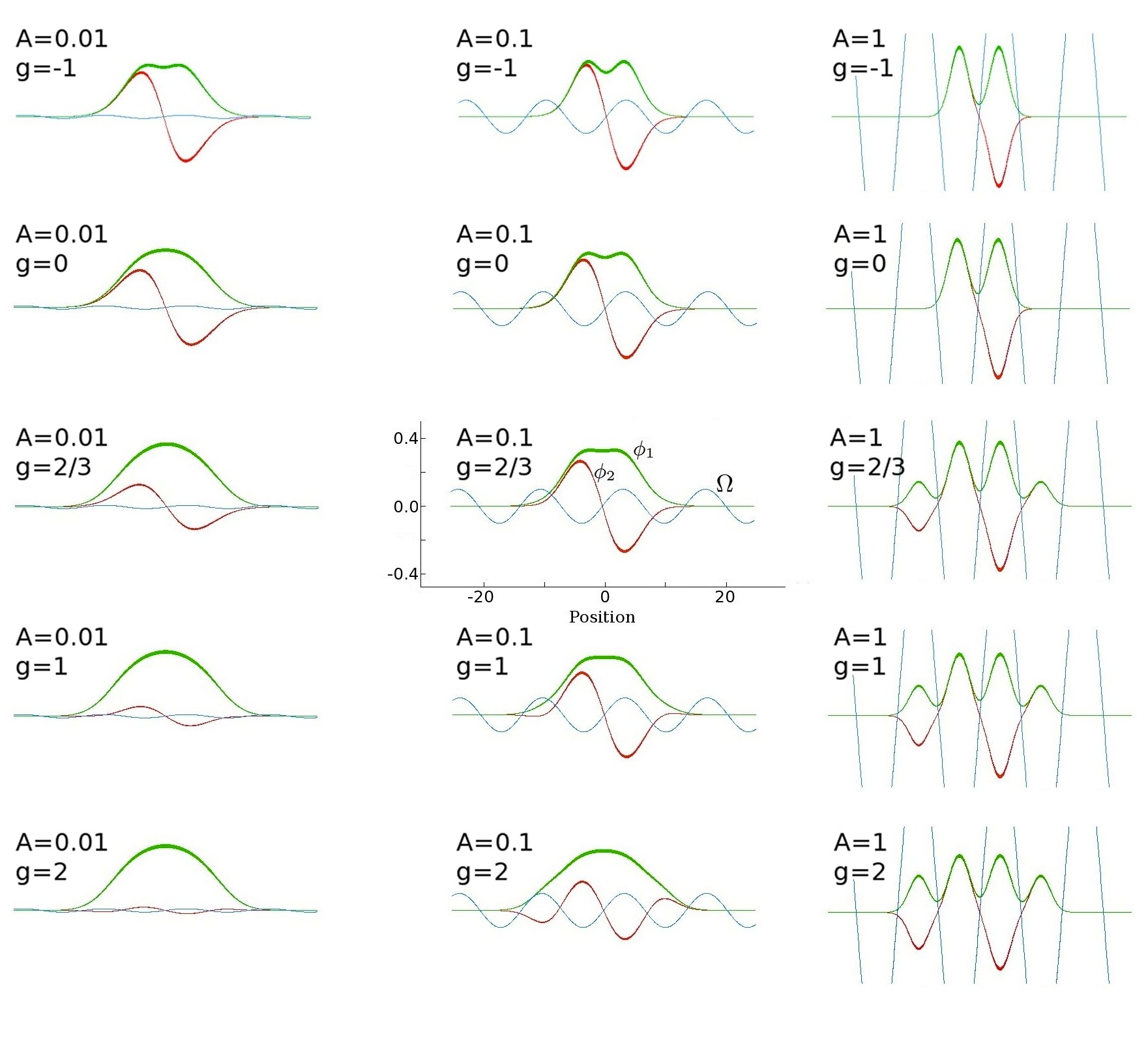
Figure 1: (Color online) Stationary wave functions $\phi_{1}(x)$ (green) and $\phi_{2}(x)$ (red) in the case of the odd modulation function, $\Omega(x)=A\sin\left(\alpha x\right)$ (blue), see Eq. (2). The left, middle and right columns correspond to the weak, moderate, and strong linear coupling, respectively, with $A=0.01$, $A=0.1$, and $A=1$. The rows running from top to bottom correspond the following values of the XPM coefficient: $g=-1,0,2/3,1,2$.

III.2 The number of kinks in the ground states

The number of kinks is the most essential overall (topological) characteristic of the GS [we stress that the kinks are always formed in one component, which is denoted $\phi_{2}(x)$, while the other component, $\phi_{1}(x)$, does not change its sign]. As said above, in the case of the odd/even spatial modulation of the linear coupling in Eqs. (3) and (2), the number of kinks is always odd/even too. Analyzing numerical data, we counted those kinks which showed, in their core areas, the amplitude of $\phi_{2}$ that would be no smaller than $5\%$ of the largest value of $\psi_{1}$. In terms of the present analysis, this actually means that the kinks were taken into account if the respective amplitude of $\phi_{2}(x)$ would not fall below $\phi_{2}=0.02$.

The number of kinks in the GS is presented, as a function of the linear-coupling strength $A$ and modulation wavenumber $\alpha$, in maps collected in Fig. 2, at four fixed values of the XPM coefficient $g$. The case of $g=-1$ is not included, as it always gives rise to a single kink, cf. Fig. 1. The latter observation is explained by the fact that the attraction between the two components, in the case of $g=-1$, impedes $\phi_{2}(x)$ to cross zero while $\phi_{1}(x)$ is not too small, except for at the central point. On the other hand, at $g>0$ the repulsion between the components facilitates the appearance of the zero crossings of $\phi_{2}(x)$, thus leading to the increase in the number of kinks. We note that the maps pertaining to different positive values of $g$, i.e., $g=2/3,$ $1$, and $2$, are not drastically different.

Quite naturally, the number of the kinks increases with the modulation wavenumber, $\alpha$, as the kinks are associated with points where $\Omega(x)$ changes its sign. The same argument explains why the number of kinks increases too with the modulation strength, $A$.

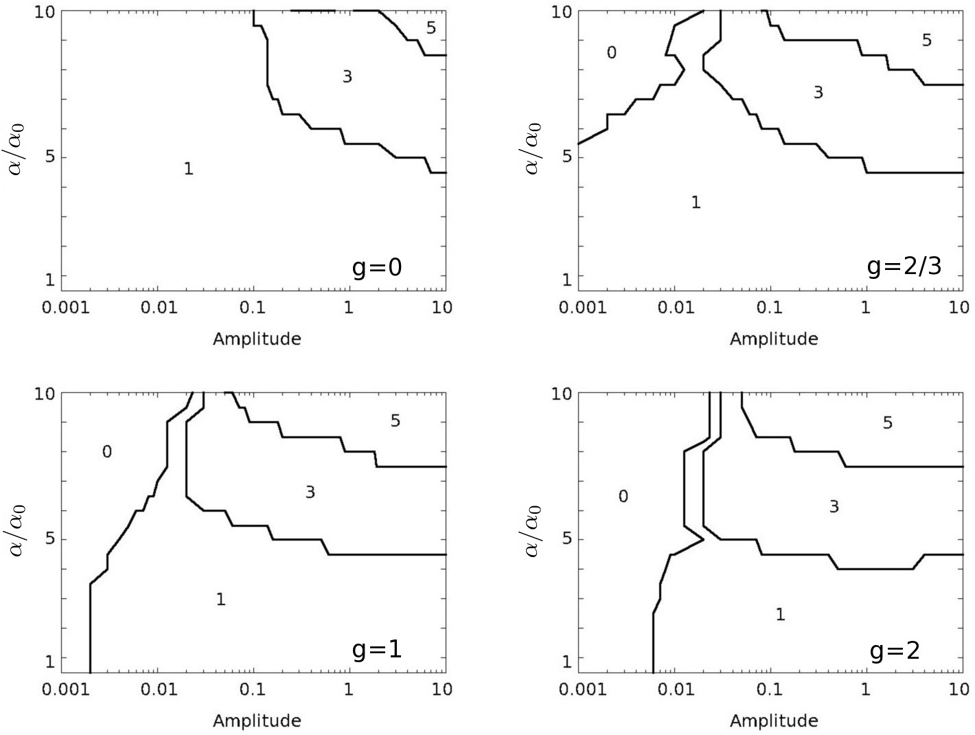
Figure 2: The number of kinks in the numerically found ground states, as a function of amplitude $A$ and normalized wavenumber $\alpha/\alpha_{0}$ (with $\alpha_{0}=0.09248$) of the odd spatial modulation of the linear coupling, see Eq. (2). The maps are displayed at four fixed values of the XPM coefficients, $g=0,2/3,1,2$. The values of $A$ are shown on the logarithmic scale, to comprise the cases of weak, moderate, and strong linear coupling. In this case of the odd modulation, the number of kinks is odd too, see the text.

Some data concerning the number of kinks has also been collected for the case of the even modulation of the local modulation, with function $\cos\left(\alpha x\right)$ in Eq. (2). The respective map is displayed in Fig. 3 for $g=0$. The absence of the kink at the central point makes their overall number smaller than in the case of the odd modulation. In this case, general features exhibited by the dependence of the number of kinks on parameters $A,\alpha$ and $g$ are qualitatively the same as in the case of the odd modulation.

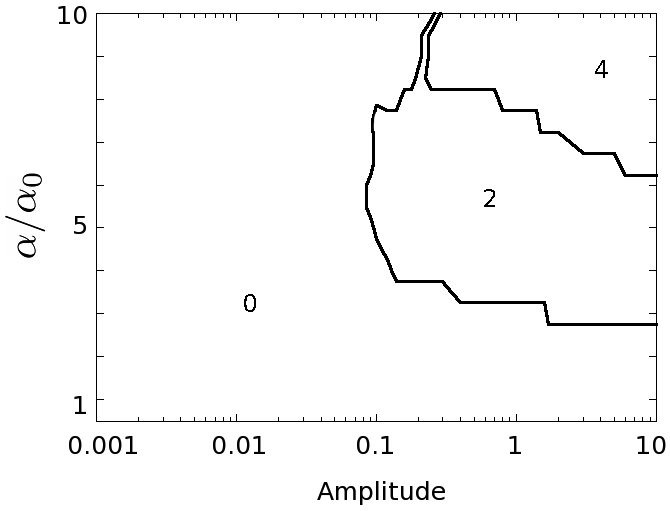
Figure 3: The same as in Fig. 3 (again, with $\alpha_{0}=0.09248$), but for the case of the even modulation function, $\cos\left(\alpha x\right)$, in Eq. (2), and $g=0$. The number of kinks is even in the case of the even modulation, see the text.

IV Conclusion

The objective of this work was to identify the GSs (ground states) in two-component models based on the system of two NLSEs/GPEs coupled by the linear interconversion and nonlinear (XPM) interaction, with the self-repulsion acting in each component. A well-known property of such systems is that their GSs may be represented by either symmetric or asymmetric states, depending on the strengths of linear and XPM couplings. In the present model, we have extended the idea of Ref. Dum and considered in detail the periodic odd, or even spatial modulation of the linear coupling, $\Omega(x)$. The repeated change of the sign by $\Omega(x)$ produces a strong impact on the structure of the GS in the two-component system, as the relative sign of the components tends to be locked to the local sign of $\Omega$. Accordingly, the GS of the trapped system features one or several kinks in one component, while the other component does not change its sign. The parity of the number of kinks coincides with that of the modulation function. The interplay of the modulation of $\Omega(x)$ with the trapping potential also strongly affects the transition between the states with nearly equal and strongly different amplitudes of the two components. These results were obtained by means of the systematic numerical analysis, and also in the analytic perturbative form. The model may be realized in nonlinear optics, in terms of periodically modulated slab waveguides. Also, it may also be implemented in BECs, when two-photon Raman transitions are used.

A challenging problem is to extend the analysis to two-dimensional binary systems, with a two-dimensional (checkerboard-patterned) modulation of the linear coupling. This two-dimensional setting may also be realized in the photonic-crystal medium. In 2D, as as already discussed in Dum , it should be possible to generate vortices and (in more complex settings) other types of topological defects. In fact, this method of vortex generation is completely analogue to the methods of creating ”artificial” magnetic fields employing spatially dependent Berry’s phase Juze , or Raman couplings Lin . Another interesting extension of the present studies is to perform a similar analysis for quantum systems, formulated in terms of an appropriate Bose-Hubbard model, i.e. in the strongly correlated limit, where one expects the appearance of quantum solitons (cf. kostia and references therein).

B.A.M. appreciates hospitality of ICFO (Institut de Ciències Fotòniques), Castelldefels (Barcelona), Spain. The work of this author was supported, in a part, by the German-Israel Foundation through grant No. 149/2006. We acknowledge also financial support from the Spanish MINCIN project FIS2008-00784 (TOQATA), Consolider Ingenio 2010 QOIT, EU STREP project NAMEQUAM, ERC Advanced Grant QUAGATUA, and from the Humboldt Foundation.

References

- (1) C. J. Myatt, E. A. Burt, R. W. Ghrist, E. A. Cornell, and C. E. Wieman, Phys. Rev. Lett. 78, 586 (1997).
- (2) L. Pitaevskii and S. Stringari, Bose-Einstein Condensation (Clarendon Press: Oxford, 2003).
- (3) D. S. Hall, M. R. Matthews, J. R. Ensher, C. E. Wieman, and E. A. Cornell, Phys. Rev. Lett. 99, 190402 (1998); K. M. Mertes, J. W. Merrill1, R. Carretero-González, D. J. Frantzeskakis, P. G. Kevrekidis, and D. S. Hall, ibid. 99, 190402 (2007).
- (4) D. M. Weld, P. Medley, H. Miyake, D. Hucul, D. E. Pritchard, and W. Ketterle, Phys. Rev. Lett. 103, 245301 (2009); C. Hamner, J. J. Chang, P. Engels , and M. A. Hoefer, arXiv:1005.2601 (2010).
- (5) S. Inouye, M. R. Andrews, J. Stenger, H. J. Miesner, D. M. Stamper-Kurn, and W. Ketterle, Nature 392, 151 (1998); M. Theis, G. Thalhammer, K. Winkler, M. Hellwig, G. Ruff, R. Grimm, and J. H. Denschlag, Phys. Rev. Lett. 93 123001 (2004).
- (6) D.M. Stamper-Kurn and W. Ketterle, Proceedings of Les Houches 1999 Summer School, Session LXXII (cond-mat/0005001) (1999).
- (7) M. Lewenstein, A. Sanpera, V. Ahufinger, B. Damski, A. Sen(De), and U. Sen”, Adv. Phys. 56, 243 (2007).
- (8) K. Eckert, L. Zawitkowski, M. J. Leskinen, A. Sanpera, and M. Lewenstein New J. Phys. 9, 133 (2007).
- (9) T. L. Ho and V. B. Shenoy, Phys. Rev. Lett. 77, 3276 (1996); E. Timmermans, ibid. 81, 5718 (1998)
- (10) M. A. Porter, P. G. Kevrekidis, and. B. A. Malomed, Physica D 196, 106 (2004).
- (11) H. J. Miesner, D. M. Stamper-Kurn, J. Stenger, S. Inouye, A. P. Chikkatur, and W. Ketterle, Phys. Rev. Lett. 82, 2228 (1999).
- (12) M. Trippenbach, K. Goral, K. Rzazewski, B. Malomed, and Y. B. Band, J. Phys. B - At. Mol. Opt. Phys. 33, 4017 (2000).
- (13) R. J. Ballagh, K. Burnett, and T. F. Scott, Phys. Rev. Lett. 78, 1607 (1997).
- (14) J. Williams, R. Walser, J. Cooper, E. Cornell, and M. Holland, Phys. Rev. A 59, R31 (1999).
- (15) D. T. Son and M. A. Stephanov, Phys. Rev. A 65, 063621 (2002).
- (16) S. D. Jenkins and T. A. B. Kennedy, Phys. Rev. A 68, 053607(2003).
- (17) Q.-H. Park and J. H. Eberly, Phys. Rev. A 70, 021602(R) (2004).
- (18) I. M. Merhasin, B. A. Malomed, and R. Driben, J. Phys. B: At. Mol. Opt. Phys. 38, 877 (2005).
- (19) S. K. Adhikari and B. A. Malomed, Phys. Rev. A 79, 015602 (2009).
- (20) G. P. Agrawal, Nonlinear Fiber Optics (Academic Press: San Diego, 1995).
- (21) E. Dulkeith, F. Xia, L. Schares, W. M. J. Green, and Y. A. Vlasov, Opt. Exp. 14, 3853 (2006); N.-C. Panoiu, B. A. Malomed, and R. M. Osgood, Jr., Phys. Rev. A 78, 013801 (2008).
- (22) S. G. Johnson, P. R. Villeneuve, S. H. Fan, and J. D. Joannopoulos, Phys. Rev. B 62, 8212 (2000); S. G. Tikhodeev, A. L. Yablonskii, E. A. Muljarov, N. A. Gippius, and T. Ishihara, ibid. 66, 045102 (2002).
- (23) A. W. Snyder, D. J. Mitchell, L. Poladian, D. R. Rowland, and Y. Chen, J. Opt. Soc. Am. B 8, 2102 (1991).
- (24) R. Dum, J.I. Cirac, P. Zoller, and M. Lewenstein, Phys. Rev. Lett. 80, 2969 (1998).
- (25) A. Aharony, Phys. Rev. B 18, 3328 (1978); B.J. Minchau and R.A. Pelcovits, Phys. Rev. B 32, 3081 (1985); D.E. Feldman, J. Phys. A 31, L177 (1998); D.A. Abanin, P.A. Lee, and L.S. Levitov, Phys. Rev. Lett. 98, 156801 (2007); G.E. Volovik, JETP Lett. 84, 455 (2006); J. Wehr, A. Niederberger, L. Sanchez-Palencia, and M. Lewenstein, Phys. Rev. B 74, 224448 (2006).
- (26) A. Niederberger, T. Schulte, J. Wehr, M. Lewenstein, L. Sanchez-Palencia, and K. Sacha, Phys. Rev. Lett. 100, 030403 (2008).
- (27) A. Niederberger, J. Wehr, M. Lewenstein, and K. Sacha, Europhys. Lett 86, 26004 (2009).
- (28) A. Niederberger, M. M. Rams, J. Dziarmaga, F. M. Cucchietti, J. Wehr, M. Lewenstein Phys. Rev. A 82, 013630 (2010).
- (29) M. L. Chiofalo, S. Succi, and M. P. Tosi, Phys. Rev. E 62, 7438 (2000).
- (30) V. P. Mineev, Zh. Eksp. Teor. Fiz. 67, 263 (1974) [English translation: Sov. Phys.—JETP 40, 132 (1974)].
- (31) G. Juzeliunas and P. Öhberg, Phys. Rev. Lett. 93, 033602, (2004);G. Juzeliunas, P. Öhberg, J. Ruseckas, and A. Klein, Phys. Rev. A 71, 053614 (2005); K.J. Günter, M. Cheneau, T. Yefsah, S.P. Rath, and J. Dalibard, Phys. Rev. A 79, 011694(R) (2009).
- (32) Y.-J.Lin, R.L. Compton, A.R. Perry, W.D. Phillips, J.V. Porto, and I.B. Spielman, Phys. Rev. Lett. 102, 130401 (2009); Y.-J.Lin, R. L. Compton, K. Jiménez-Garcıa, J.V. Porto, and I.B. Spielman, Nature 462, 628 (2009).
- (33) K.V. Krutitsky, J. Larson, and M. Lewenstein, submitted to Phys. Rev. A., arXiv:0907.0625.