Mass reconstruction by gravitational shear and flexion

Abstract

Aims. Galaxy clusters are considered as excellent probes for cosmology. For that purpose, their mass needs to be measured and their structural properties needs to be understood.

Methods. We propose a method for galaxy cluster mass reconstruction which combines information from strong lensing, weak lensing shear and flexion. We extend the weak lensing analysis to the inner parts of the cluster and, in particular, improve the resolution of substructure.

Results. We use simulations to show that the method recovers the mass density profiles of the cluster. We find that the weak lensing flexion is sensitive to substructure. After combining the flexion data into the joint weak and strong lensing analysis, we can resolve the cluster properties with substructures.

1 Introduction

Galaxy clusters are the most massive virialized structures in the universe, and are considered as valuable probes for cosmological parameters. From numerical simulations one can identify collapsed structures (called halos) and study their properties. In $\Lambda$CDM simulation, the density profile of halos has a universal form, closely following the NFW profile (Navarro et al. 1996). Moreover, numerical simulations predict a rich population of sub-clumps within the virial radius of the main halo.

Weak gravitational lensing provides a powerful tool for studying the mass distribution of clusters of galaxies as well as the large-scale structure in the Universe (see Bartelmann & Schneider 2001; Refregier 2003; Schneider et al. 2006; Munshi et al. 2008, for reviews on weak lensing). Several methods were developed on cluster mass reconstructions (see e.g. Kaiser & Squires 1993; Seitz & Schneider 2001). Besides weak lensing, strong lensing systems are also employed to extend the weak lensing analysis into the inner part of clusters, such as the multiply-imaged systems and the corresponding identification of the location of critical curves (Cacciato et al. 2006; Bradač et al. 2005b). Since then some cluster mass reconstructions have been successfully carried out (Bradač et al. 2005a, 2006; Merten et al. 2009). Both methods reconstruct the gravitational potential $\psi$, based on minimizing a $\chi^{2}-$function comparing observed data with model (Bartelmann 1996; Seitz et al. 1998).

Flexion has been recently studied as the derivative of the shear, and responds to small-scale variations in the gravitational potential (Goldberg & Natarajan 2002; Goldberg & Bacon 2005; Bacon et al. 2006). The two complex spin-1 and spin-3 components of flexion together with the shear describe how intrinsically round sources are mapped into ‘arclets’. The measurement of flexion can be obtained in principle from the same imaging data as used for shear measurements, and methods for that have been discussed in the literature (Irwin & Shmakova 2006; Okura et al. 2007; Goldberg & Leonard 2007; Schneider & Er 2008). One disadvantage of shear technique is that galaxies have a broad intrinsic ellipticity distribution which constitutes a serious noise component. Since third-order brightness moments of galaxies are suspected to be much smaller than second-order ones, we expect a lower intrinsic noise in flexion measurements. It has been noted that flexion can contribute to study the galaxy and cluster halo mass and density profiles, and particularly sensitive to substructure (Bacon et al. 2009; Leonard et al. 2009; Okura et al. 2008). Okura et al. (2008); Leonard et al. (2007) have used flexion measurements to detect substructure in Abell 1689.

We propose a method that combines shear measurements and flexion into a weak lensing mass reconstruction, which enable us to reconstruct the mass distribution of a lens with special sensitivity to substructure. It is based on an estimations of the lensing potential using $\chi^{2}$-minimization. The resulting equations are first linearzied and then solved by iteration. We outline the basic lensing formalism in Sect. 2, and the ideas of reconstruction method in Sect. 3 (calculations are shown in the Appendix). Numerical tests are presented in Sect. 4, and conclusions are given in Sect. 5.

2 Basic formalism

We mainly follow the notations of Schneider & Er (2008) to present the basic gravitational lensing shear and flexion formalism. We adopt the thin lens approximation where the lensing mass distribution is projected onto the lens plane. Thus, all the lensing properties are contained in the lensing potential $\psi$, which is the projected Newtonian gravitational potential on the lens plane

$$\psi(\mbox{\boldmath$\theta$})={1\over\pi}\int_{\Re^{2}}{\mathrm{d}}^{2}\theta^{\prime}\kappa(\mbox{\boldmath$\theta$}^{\prime}){\rm ln}|\mbox{\boldmath$\theta$}-\mbox{\boldmath$\theta$}^{\prime}|\;,$$ (1)

where $\theta$ denotes the (angular) position in the lens plane, and $\kappa(\mbox{\boldmath$\theta$})$ is the projected mass density $\Sigma(\mbox{\boldmath$\theta$})$ of the lens in units of

$$\Sigma_{\rm cr}={c^{2}\over 4\pi G}{D_{\infty}\over D_{\rm d}D_{\rm d,\infty}},\;\;{\rm so}\;\;\kappa(\mbox{\boldmath$\theta$})={\Sigma(\mbox{\boldmath$\theta$})\over\Sigma_{\rm cr}}$$ (2)

for a fiducial source located at a redshift $z\rightarrow\infty$. Here $D_{\infty},D_{\rm d}$ and $D_{\rm d,\infty}$ are the angular diameter distances between the observer and the source, the observer and the lens and between the lens and the source, respectively. The second-order local expansion of the lensing equation in Cartesian coordinates reads $\beta_{i}=\theta_{i}-\psi_{,ij}\theta_{j}-\psi_{,ijk}\theta_{j}\theta_{k}/2$, where indices separated by a comma denote partial derivatives with respect to $\theta_{i}$, and the Einstein summation convention is used. The surface mass density $\kappa$ and the complex shear $\gamma=\gamma_{1}+{\rm i}\gamma_{2}$ are given in terms of the deflection potential through

$$\kappa=(\psi_{,11}+\psi_{,22})/2,\;\gamma=(\psi_{,11}-\psi_{,22})/2+{\rm i}\psi_{,12}\;.$$ (3)

The two flexions ${\cal F},{\cal G}$ are combinations of third-order derivatives of $\psi$, and also related to the gradient of $\kappa$ and $\gamma$

$${\cal F} = {1\over 2}\left[\psi_{,111}+\psi_{,122}+{\rm i}\left(\psi_{,112}+\psi_{,222}\right)\right]\;;$$

$${\cal G} = {1\over 2}\left[\psi_{,111}-3\psi_{,122}+{\rm i}\left(3\psi_{,112}-\psi_{,222}\right)\right]\;,$$

$${\cal F} = \nabla_{\rm c}\kappa=\nabla_{\rm c}^{*}\gamma,\;{\cal G}=\nabla_{\rm c}\gamma,$$ (4)

where we defined the differential operators

$$\nabla_{\rm c}={\partial\over\partial\theta_{1}}+{\rm i}{\partial\over\partial\theta_{2}};\;\nabla_{\rm c}^{*}={\partial\over\partial\theta_{1}}-{\rm i}{\partial\over\partial\theta_{2}}.$$

The second-order lensing equation in complex notation then reads

$$\beta=(1-\kappa)\theta-\gamma\theta^{*}-{1\over 4}{\cal F}^{*}\,\theta^{2}-{1\over 2}{\cal F}\,\theta\theta^{*}-{1\over 4}{\cal G}\,(\theta^{*})^{2}\;.$$ (5)

Due to the mass-sheet degeneracy in lensing system (see, e.g., Falco et al. 1985; Schneider & Seitz 1995) the lens equation is rewritten in reduced form as (see Schneider & Er 2008)

$$\hat{\beta} \equiv {\beta\over(1-\kappa)}$$

$$= \theta-g\theta^{*}-\Psi_{1}^{*}(G_{1})\,\theta^{2}-2\Psi_{1}(G_{1})\,\theta\theta^{*}-\Psi_{3}(G_{1},G_{3})\,(\theta^{*})^{2}\;,$$

where $g,G_{1},G_{3}$ are the reduced shear and the reduced flexion components,

$$g = {\gamma\over 1-\kappa}\;;$$

$$G_{1} \equiv \nabla_{\rm c}^{*}g={{\cal F}+g{\cal F}^{*}\over(1-\kappa)}\;;$$

$$G_{3} \equiv \nabla_{\rm c}g={{\cal G}+g{\cal F}\over(1-\kappa)}\;,$$ (7)

and where $\Psi_{1},\Psi_{3}$ are given by

$$\Psi_{1} = {G_{1}-gG_{1}^{*}\over 4(1-gg^{*})},$$

$$\Psi_{3} = {G_{3}\over 4}-{g(G_{1}-gG_{1}^{*})\over 4(1-gg^{*})}\;.$$ (8)

All the relation above are written for sources located at redshift $z\rightarrow\infty$. For a source at redshift $z$ and lens at redshift $z_{\rm d}$, the lensing strength is reduced by multiplying $\psi$ (and all its derivatives) by a ‘cosmological weight’ function,

$$Z(z)\equiv\left[D_{\rm d,\infty}\over D_{\infty}\right]^{-1}{D_{\rm ds}\over D_{\rm s}}H(z-z_{\rm d}),$$ (9)

where $D_{\rm ds}$ and $D_{\rm s}$ are the angular diameter distances between the lens and the source, and the observer and the source. $H(z-z_{\rm d})$ is the Heaviside step function to give zero weight to sources located in front of the lens. Thus, at redshift $z$

$$\kappa(z) = Z(z)\kappa,\,\gamma(z)=Z(z)\gamma,$$

$${\cal F}(z) = Z(z){\cal F},\,{\cal G}(z)=Z(z){\cal G}.$$ (10)

Information about the lensing potential can be obtained through the reduced shear and reduced flexion by measuring the ellipticity $\epsilon$ and the higher-order brightness moments, or called HOLICs (Okura et al. 2007). The information on the lens potential is contained in the transformation between the source and image ellipticity

$$\epsilon^{\rm s}=\begin{cases}\dfrac{\epsilon-g}{1-g^{*}\epsilon}\quad{\rm for}\;\bigl{\lvert}g\bigr{\rvert}<1;\\[15.00002pt] \dfrac{1-g\epsilon^{*}}{\epsilon^{*}-g^{*}}\quad{\rm for}\;\bigl{\lvert}g\bigr{\rvert}>1,\\ \end{cases}$$ (11)

and the higher-order brightness moments

$$T_{1}^{\rm s} \approx T_{1}-{9F_{0}-12Q_{0}^{2}\over 4}G_{1},$$

$$T_{3}^{\rm s} \approx T_{3}-{3F_{0}\over 4}G_{3},$$ (12)

where $Q,T,F$ are the second-, third- and fourth- order brightness moments, respectively (see Schneider & Er 2008, for definitions), the superscript ^s indicates source quantities, and the subscript indicates the spin of the moments. If we assume that the ensemble average of intrinsic moments vanish, $\langle\epsilon^{s}\rangle=0$, $\langle T_{1,3}^{\rm s}\rangle=0$, the expectation value for the galaxy image quantities yields the estimator of reduced shear and reduced flexion

$$g=\begin{cases}\bigl{\langle}\epsilon\bigr{\rangle}\quad{\rm if}\;|g|<1,\\[10.00002pt] \bigl{\langle}{1/\epsilon^{*}}\bigr{\rangle},\quad{\rm otherwise},\\ \end{cases}$$ (13)

$$G_{1} \approx t_{1}=\left\langle{4\over 9F_{0}-12Q_{0}^{2}}T_{1}\right\rangle;$$

$$G_{3} \approx t_{3}=\left\langle{4\over 3F_{0}}T_{3}\right\rangle.$$ (14)

Here we use $t_{1,3}$ to indicate the estimators of the reduced flexion. These estimates of reduced shear and reduced flexion break down when the image is located on or close to a critical curve.

3 Mass reconstruction method

The strategy of our method is similar to that of the strong- and weak-lensing united method (Bradač et al. 2005b, a). Thus, we include flexion in the reconstruction of the lensing potential $\psi$. There are two reasons for combining shear and flexion other than using flexion alone in the mass reconstruction. In current observations, the number density of images from which flexion can be estimated is low, as we can see in our simulation data. Even with future higher flexion number density surveys, flexion is most sensitive to substructures, but rather insensitive to the larger-scale (cluster-scale) smooth potential.

3.1 The $\chi^{2}$-function

We describe the cluster mass distribution by the deflection potential $\psi$ on a regular grid, use finite differencing to calculate the deflection angle, the reduced shear and the flexion. These quantities on the grid are considered to describe the lens model which can be compared with data. Our aim is to seek a potential ${\psi}$ that minimizes the difference between model ($g,G_{1},G_{3}$) and data ($\epsilon,t_{1},t_{3}$). We therefore define a $\chi^{2}$-function

$$\chi^{2}(\psi)=\chi^{2}_{s}(\psi)+\chi^{2}_{\epsilon}(\psi)+\chi^{2}_{f}(\psi)+\eta R(\psi),$$ (15)

where $\chi^{2}_{s}$, $\chi^{2}_{\epsilon}(\psi)$ and $\chi^{2}_{f}(\psi)$ contain the information from strong lensing multiple image systems, shear and flexion, respectively. $\eta R$ is a regularization term, used to smooth out small-scale noise components, i.e., to avoid overfitting the data. For a multiple image system with $N_{m}$ images located at $\mbox{\boldmath$\theta$}_{m}$, the $\chi^{2}_{s}$ term is well defined by Bradač et al. (2005b)

$$\chi^{2}_{s}=\sum_{\rm str}\sum_{m=1}^{N_{m}}b_{m}^{T}S^{-1}b_{m},$$ (16)

where $\sum_{\rm str}$ is the sum over all strong lens system, and $\mbox{\boldmath$b$}_{m}=\mbox{\boldmath$\theta$}_{m}-\mbox{\boldmath$\alpha$}(\mbox{\boldmath$\theta$}_{m})-\mbox{\boldmath$\beta$}_{s}$. $\mbox{\boldmath$\beta$}_{s}$ is the average source position, and $S$ is the covariance matrix $S={\rm diag}(\sigma^{2}_{s1},\sigma^{2}_{s2})$. The shear term $\chi^{2}_{\epsilon}$ is

$$\chi^{2}_{\epsilon}=\sum^{N_{\rm g}}_{i=1}{|\epsilon_{i}-g(\mbox{\boldmath$\theta$},z_{i})|^{2}\over\sigma_{\epsilon}^{2}},$$ (17)

where $N_{\rm g}$ is the number of background galaxies, and

$$\sigma_{\epsilon}^{2}=\left(1-|g|^{2}\right)^{2}\sigma_{\epsilon^{s}}^{2}+\sigma_{\rm err}^{2},$$ (18)

with $\sigma_{\epsilon^{s}}\approx 0.3$ is the standard deviation (Brainerd et al. 1996), $\sigma_{\rm err}$ is the measurement error, which we take 0.1 in this paper, and $g$ is the reconstructed reduced shear.

The flexion term is defined in a way similar to the shear

$$\chi^{2}_{f}=\sum^{N_{f}}_{i=1}\left({|t_{1i}-G_{1}(\mbox{\boldmath$\theta$}_{i},z_{i})|^{2}\over{\sigma_{t1}^{2}}}+{|t_{3i}-G_{3}(\mbox{\boldmath$\theta$}_{i},z_{i})|^{2}\over\sigma_{\large t3}^{2}}\right),$$ (19)

where $G_{1,3}$ are the reduced flexions at position $\mbox{\boldmath$\theta$}_{i}$ and redshift $z_{i}$ in our model. Note that we can measure only the reduced flexion. There is a significant difference between the reduced flexion and its approximation ${\cal F}/(1-\kappa)$ or ${\cal G}/(1-\kappa)$ in the region where the shear is not small. However, the definition of reduced flexion (Eq.7) renders the $\chi^{2}_{f}$ function (Eq.19) complicated and the equations become difficult to solve. We thus define

$$G_{1}^{\prime}\equiv{{\cal F}\over 1-\kappa};\;\;\;G_{3}^{\prime}\equiv{{\cal G}\over 1-\kappa}.$$ (20)

From Eq.(7) it is easy to obtain

$$G_{1}^{\prime}={G_{1}-gG_{1}^{*}\over 1-gg^{*}};\;\;\;G_{3}^{\prime}=G_{3}-gG_{1}^{\prime}.$$ (21)

We thus use a modified estimator for the observed reduced flexion,

$$t_{1}^{\prime}={t_{1}-\epsilon t_{1}^{*}\over 1-\epsilon\epsilon^{*}};\;\;\;t_{3}^{\prime}=t_{3}-\epsilon t_{1}^{\prime},$$ (22)

and replace $t_{1}$, $t_{3}$ by $t_{1}^{\prime}$, $t_{3}^{\prime}$ in (Eq.19). The flexion term $\chi^{2}_{f}$ is thus redefined as

$$\chi^{2}_{f}=\sum^{N_{f}}_{i=1}\left(\dfrac{\left|\dfrac{{\cal F}_{i}}{1-\kappa_{i}}-t^{\prime}_{1i}\right|^{2}}{\sigma_{t1^{\prime}}^{2}}+\dfrac{\left|\dfrac{{\cal G}_{i}}{1-\kappa_{i}}-t^{\prime}_{3i}\right|^{2}}{\sigma_{t3^{\prime}}^{2}}\right).$$ (23)

The $\sigma^{2}_{t1^{\prime}}$ and $\sigma^{2}_{t3^{\prime}}$ are different from the dispersion in flexion measurement or intrinsic flexion variance, which are both difficult to obtain from current observations. In Goldberg & Leonard (2007), the intrinsic scatter of flexion are estimated as $\sigma_{a|{\cal F}|}=0.03$ and $\sigma_{a|{\cal G}|}=0.04$, where $a$ is the semi-major axis of the lensed image, so that the combination $a|\cal F|$ represents a dimensionless term. Hawken & Bridle (2009); Leonard et al. (2009) used a conservative estimate $\sigma_{\cal F}=0.1/^{\prime\prime}$. Here we use

$$\sigma^{2}_{t1^{\prime}}=\left|{\partial G_{1}^{\prime}\over\partial g}\right|^{2}\sigma^{2}_{\epsilon}+\sigma^{2}_{t1};$$

$$\sigma^{2}_{t3^{\prime}}=\left|{\partial G_{3}^{\prime}\over\partial g}\right|^{2}\sigma^{2}_{\epsilon}+\sigma^{2}_{t3},$$ (24)

where $\sigma_{t1}$, $\sigma_{t3}$ are the dispersion of flexion data. The first term on the right is scatter due to intrinsic ellipticity and shear measurement error.

In principle, the total number of flexion measurements is the same as the number of galaxy images $N_{f}=N_{g}$ from which shear can be estimated. But in reality, flexion is measurable only for a subset of (larger) images; beside that, we discard low signal-to-noise flexion measurements. Thus the number of images from which flexion can be estimated is usually smaller than the number of galaxy images with shear measurements.

To find the minimum $\chi^{2}$-function, we solve the set of equations

$${\partial\chi^{2}(\{\psi_{i}\})\over\partial\psi_{i}}=0,$$ (25)

which is in general a non-linear set of equations. This problem is solved by an iterative procedure (Bradač et al. 2005b). We perform a three-level iteration process, start with initial model $\kappa^{0}$ as the fixed regularization, linearize the system (Appendix), solve the linear system of equations as the inner-level. These steps are repeated until convergence of $\kappa$ is achieved. The middle-level is repeating the inner level with new regularization, based on the estimate of $\kappa$ from previous step result, until we can get $\chi^{2}_{\rm red}\sim 1$. Finally we increase the number of grid points in the field and repeat the first two level iterations on the new grid until we reach the final desired grid spacing, i.e., resolution.

For the regularization we choose

$$R=\sum_{i,j=1}^{N_{x},N_{y}}\left[\kappa_{ij}^{(n)}-\kappa^{(n-1)}(\mbox{\boldmath$\theta$}_{ij})\right]^{2},$$ (26)

where $\kappa^{(n)}$ and $\kappa^{(n-1)}$ are current and previous resulting $\kappa$ map in every middle-level. For the first step, we can use an initial model $\kappa^{(0)}$ which is obtained from other methods, or simple set $\kappa^{(0)}=0$ across the whole field.

3.2 Grid point field

Finite differencing techniques (Abramowitz & Stegun 1972) provide a way to calculate $\kappa$ and $\gamma$ on the potential $\psi$ grid field. We need 9 grid points for second-order derivatives required for $\kappa$ and $\gamma$, and 16 points for flexion. But by using $4\times 4$ points, one would obtain the flexion value at the center of a grid cell. Thus we instead use $5\times 5$ finite difference scheme to obtain the flexion on the grid. For instance,

$${\cal F}_{1}(i,j)={1\over 12\Delta^{3}}\sum^{+2}_{\Delta_{i},\Delta_{j}=-2}W_{\Delta_{i},\Delta_{j}}\psi(i+\Delta_{i},j+\Delta_{j}),$$ (27)

where the coefficients $W_{\Delta_{i},\Delta_{j}}$ used for spin-1 flexion are given in the left panel of Fig. 1. Bilinear interpolation can be used to obtain the shear and flexion for an arbitrary position in the field. We need to extend two grid rows and columns on each boundary of the entire field, which means we use a $(N+4)^{2}$ grid to perform the method for inner $N^{2}$ grid. Note that the flexion drops quickly with increasing distance from the cluster center, so that there is few images with flexion signal near the grid boundary.

Since shear and flexion are second- and third-order derivatives of $\psi$, the potential field is not fixed with shear and flexion constraints alone. However, $\kappa$ is unchanged under the transformation $\psi(\mbox{\boldmath$\theta$})\to\psi(\mbox{\boldmath$\theta$})+\psi_{0}+\mbox{\boldmath$\alpha$}\cdot\mbox{\boldmath$\theta$}$, where $\psi_{0}$ and $\alpha$ are arbitrary constants. We leave the constants free to simplify the numerical solution. The mass-sheet degeneracy transformation of the potential is given by $\psi\to\psi^{\prime}=(1-\lambda)\theta^{2}/2+\lambda\psi$, which does not affect the reduced shear and reduced flexion, but affects $\kappa$ as

$$\kappa^{\prime}=(1-\lambda)+\lambda\kappa,$$ (28)

which we call the $\lambda$ transformation. We will take advantage of this transformation for adjusting $\kappa$ later. We note that the mass-sheet transformation is exact only for all sources being located at the same redshift; for a redshift distribution, the mass-sheet degeneracy is broken. However, this breaking is not very strong, as long as no multiple images of sources with very different redshifts are considered (see Bradač et al. 2005b)

${\cal F}_{1}\to 1/(12\Delta^{3})$

${\cal G}_{1}\to 1/(8\Delta^{3})$

Figure 1: The finite differencing coefficients of ${\cal F}_{1}$(left) and ${\cal G}_{1}$(right). The coefficients of ${\cal F}_{2}$(${\cal G}_{2}$) are the same as that of ${\cal F}_{1}$(${\cal G}_{1}$) after rotating by $\pi/2$ anticlockwise(clockwise).

4 Numerical test of field properties

4.1 NIS model

First we perform our method on a Non-singular Isothermal Sphere model. The data is generated on a $40\times 40$ grid potential field with

$$\psi(\theta)={\theta_{\rm E}\over 2}\sqrt{\theta^{2}+\theta_{c}^{2}}+{\theta_{\rm E}\theta_{c}\over 2}{\rm ln}\left(\sqrt{\theta^{2}+\theta_{c}^{2}}-\theta_{c}\over\theta\right),$$ (29)

where $\theta_{\rm E}=1$ arcmin and $\theta_{c}=0.2$ arcmin. The reduced shear and reduced flexion are calculated by finite differencing. To ensure that no strongly lensed objects are included, we reject all the data points of which the absolute value of the reduced shear is larger than 0.9. Fig. 2 shows the original and reconstructed radial $\kappa$ and $|g|$ profiles. The value is obtained by annular bin average on the grid field, the origianl one as well as the reconstructed one. The small fluctuations of the results around the input profile is mainly due to noise and low grid resolution. In the left panel, we plot the convergence $\kappa$ after applying the $\lambda$ transformation Eq.28. We can see that convergence is well recovered for large $\theta$, up to the vertical line. For smaller $\theta$, the results from shear alone deviate strongly from the input. However, using shear and flexion together significantly improves the resulting mass profile. In the right panel, the absolute value of the reduced shear is shown, which is not affected by mass-sheet degeneracy. Both results, from shear alone and from combining shear and flexion show agreement with the input model. Again for small $\theta$, the result from the combined shear and flexion data gives better agreement with the input line.

Figure 2: Radial profile of the NIS cluster, the solid line is the input model, the plus points are the reconstructed result with weak lensing shear only, and the cross points are the result with weak lensing shear and flexion. The mock data is generated out of the vertical line. Left panel: convergence $\kappa$ after $\lambda$ transformation, Right panel: the absolute value of reduced shear $|g|$, all for a source at $z_{s}\to\infty$.

4.2 Mock data

Our mock data uses a cluster taken from N-body simulations by Jing & Suto (2002); Jing (2002). The cluster is simulated in the framework of a $\Lambda$CDM model with $\Omega_{\Lambda}=0.7$, $\Omega_{\rm m}=0.3$, the normalization of power spectrum $\sigma_{8}=0.9$ and Hubble constant $H_{0}=70{\rm km\,s^{-1}Mpc^{-1}}$. Dark matter halos are identified with the friends-of-friends method using a linking length equal to 0.2 times the mean particle separation. The halo mass $M$ is defined as the mass enclosed within the virial radius according to the spherical collapse model (Kitayama & Suto 1996; Bryan & Norman 1998; Jing & Suto 2002). The virial mass of the cluster which we use here is $3.4\times 10^{14}{\rm h^{-1}}M_{\odot}$ and its redshift is $z_{\rm d}=0.326$. The particles within a box with side length of 2 virial radii were projected onto the lens plan. The surface densities are calculated using the smoothed particle hydrodynamics smoothing algorithm (Monaghan 1992) on a $4096\times 4096$ grid. The lensing potential is obtained using the fast Fourier transform method (Bartelmann et al. 1998).

A finer grid 0.1 arcsec resolution is created around the cluster center with side length of 4 arcmin. We obtain the mapping $\mbox{\boldmath$\beta$}(\mbox{\boldmath$\theta$})$ from the lens equation for each grid point and the corresponding second-order derivatives using cubic spline interpolation. We perform cubic spline interpolation again to the second-order derivatives to get the third-order derivatives. The background sources are located at random position in the source planes, and their redshifts follow a Gamma distribution

$$p(z)=\frac{z^{2}}{2\>z_{0}^{3}}\exp\left(-z/z_{0}\right)\;,$$ (30)

where $z_{0}=1/3$. The peak is at $z=2/3$ and the mean redshift is $\langle z\rangle=3z_{0}=1$. The Newton-Raphson method is used to find the corresponding images position on the image plane. The reduced shear and flexion for each image were linear interpolated using four nearest grid points.

One simulated cluster with two different projection directions is used to generate the two different sets of mock data (Fig. 3). We name the two sets of data as d02 and d03. All of the reduced shear data is used in our calculation, but for flexion, we only consider reduced flexion with absolute value in the range from 0.01 to 0.5. For higher values, merging of multiple images most likely render any flexion measurement impossible (in fact, there the whole concept of flexion break down – see Schneider & Er 2008). On the other hand, very small values of the reduced flexion are exceedingly difficult to measure and would contribute very little information due to the low signal-to-noise.

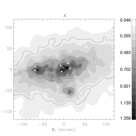
Figure 3: The convergence map of two simulated cluster used for generating mock strong lensing multiple images, weak lensing shear and flexion data. The triangles denote the image positions of multiple image systems which we use for the reconstruction. $\kappa$ is plotted for sources at $z_{s}\to\infty$, given in linear gray-scale and contours. We name the left panel cluster d02 and the right one cluster d03.

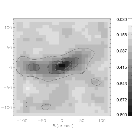
Figure 4: $\kappa$-maps obtained from shear and flexion reconstruction of the mock data cluster d02 after the $\lambda$ transformation (Eq.28), where $\lambda$ is chosen to yield the smallest $D^{2}$ (Eq.31). The left panel shows the result using $N_{\rm g}=1000$ shear galaxies and 3 multiple image systems, while in the right panel we add 89 flexion values.

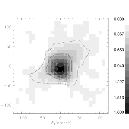
Figure 5: Reconstructed $\kappa$-maps from mock data cluster d03 after the $\lambda$ transformation. Left panel shows the result using $N_{\rm g}=$ 1000 shear galaxies, and 3 multiple image systems, whereas the right panel also uses 60 flexion values.

4.3 Reconstructed $\kappa$ map

The two mock catalogues are used to test the performance of our method. We start with an initial $20\times 20$ grid, increase $N_{x}$ and $N_{y}$ by one for each outer loop iteration, up to a $30\times 30$ grid. We use $N_{\rm g}=1000$ weak lensing galaxy images in each reconstruction, which is an accessible background galaxy number density of $\sim$ 60 images arcmin^-2. The result of the reconstructions are shown in Fig. 4 for d02 and Fig. 5 for d03. The initial regularization parameter is set to $\eta=200$ for cluster d02, and $\eta=300$ for cluster d03, and is increased by a factor of 10 for each outer-level iteration. It is usually better to set high $\eta$ and allowing $\kappa$ to change slowly. Since our reconstruction is done in a three-level iteration, and in each step we ensure $\chi^{2}/N_{\rm dof}\sim 1$, the method can successfully adapt to the data and the results are not sensitive to the initial choice of $\eta$. We need also an initial $\kappa^{0}$ field for the regularization. A simple model $\kappa^{0}=0.01$ is used here. We have also performed additional reconstructions with different initial models, and found the results are nearly independent of the initial $\kappa^{0}$, but a more realistic model allows for a faster convergence.

The number of flexion values that we used for the two cluster is different. We obtained 89 reduced flexion value between 0.01 to 0.5 in d02 (Fig. 4), and 60 that for d03 (Fig. 5). Since there is more significant extended structure in cluster d02 than in d03, we found that there are more high flexion signal data (the absolute value of the spin-1 reduced flexion greater than 0.01) in cluster d02 than that in cluster d03.

The results show that our method can reproduce the main properties of the projected mass distribution of both clusters, and is especially powerful in resolving the substructure. Fig. 4 shows that our method can reconstruct the $\kappa$ map by combining multiple images, weak lensing shear and flexion data for cluster d02. Unfortunately we cannot clearly distinguish local small-scale maxima which are due to noise from the true low-mass substructure, even with the help of flexion, like the one in the bottom corner of Fig. 4. However we can see that after including flexion, the halos become more peaky and more massive substructures are resolved and at the correct positions. In Fig. 5 it is encouraging to see that besides the overall mass distribution of the cluster halo, our method can resolve the small clumps after including flexion data. The small clump is not very significant even in the input convergence (Fig. 3), which is at a resolution of $400\times 400$. We also performed additional tests in which we use different sets of weak lensing shear and flexion data for both clusters and confirmed the validity of our method. In some cases of cluster d03 data, the shape properties can be better reconstructed and the small clump can be clearly resolve, but the position of the small clump can have an offset up to 10 arcsec from its real position. In some other realizations, the small clump cannot be clearly resolved, which is due to the noise and local low background image density around the small clump.

As an additional test, we calculate the difference $D^{2}$ between our reconstruction and the input $\kappa$, which is defined as

$$D^{2}={1\over N^{\prime}}\sum_{i,j}^{N^{\prime}}|\kappa_{ij}-\kappa_{ij}^{\rm(input)}|^{2},$$ (31)

where $N^{\prime}$ is number of grid points which are not inside the critical curves. We apply the $\lambda$ transformation (Eq.28) to the convergence results, choosing $\lambda$ such as to yield the smallest difference $D^{2}$. For cluster d02, the $D^{2}_{\rm sw}$ of the result from shear only is 0.0086, and when including flexion, it becomes 0.0085. For cluster d03, $D^{2}_{\rm sw}=0.0077$ and $D^{2}_{\rm swf}=0.0066$, respectively. Whereas we have employed the multiple image systems in our reconstruction, in cases where such strong lensing systems are not available the relative improvement obtained by the inclusion of flexion is expected to be considerable larger.

We also enlarged the allowed range for flexion to $[0.001,0.5]$ and find that in some cases, $D^{2}$ becomes larger after including flexion. After checking our resulting $\kappa$ on all grids, we identify the points which give larger $D^{2}$ after combining the flexion signal. We are aware that the relation of the reduced flexion and the reduced shear (Eq.22) can transfer extra noise from shear into flexion, especially in case of large intrinsic shear noise. In brief, if we decrease the threshold of flexion and use more data with lower signal-to-noise. The minimizing of $\chi^{2}$ will relatively lose the constrain on the region with strong flexion signal, thus a bigger $D^{2}$ is obtained.

Finally a word on the dispersion of flexion $\sigma_{t}^{\prime}$. This is a difficult parameter to determine at the moment, since we have little knowledge about the noise behavior in flexion measurement. The one we used in this paper (Eq.24) has a problem: as pointed out by Bacon et al. (2009), the flexion variance is biased by the content of substructure. Moreover, we noticed that the $\sigma_{t^{\prime}}$ we used is underestimated, it can be seen from following: $\chi^{2}_{f}/N_{f}$ is significant smaller than 1, i.e. $\sigma_{t^{\prime}}$ is too large and the constrain from flexion is lose and down weighted. If we apply more steps of iteration, the noise might be over fitted. In that case, the cluster becomes very peaky, and looks like being truncated at some edge region. Some other forms for $\sigma_{t}^{\prime}$ have been also tested, e.g. in analogy to the shear

$$\sigma^{2}_{t^{\prime}}=\left(1-(\theta_{0}|t^{\prime}|)^{2}\right)^{2}\sigma^{2}_{t^{s}}+\sigma^{\prime 2}_{\rm err},$$ (32)

where $\theta_{0}$ is size of the image. We can easily see that this $\sigma_{t^{\prime}}$ is not independent of image size and $\sigma^{\prime}_{\rm err}$ is different from that of shear (Eq.18), since it is not dimensionless. It turns out that flexion is underestimated, of which the parameter we used is $\sigma_{t^{s}}=0.1/^{\prime\prime}$ and $\sigma^{\prime}_{\rm err}=0.1/^{\prime\prime}$. Thus, flexion variance will affect the constraint of flexion. A more suitable model of flexion noise need to be constructed.

5 Conclusions

In this paper we propose a method for projected cluster mass reconstruction, which combines strong, weak lensing shear and flexion data. The method is based on a least-$\chi^{2}$ fitting of the lensing potential $\psi$ (Bradač et al. 2005b; Cacciato et al. 2006). The particular strength of this method is that the flexion data provides more information to the inner parts of the cluster and on substructure.

We test the performance of the method on our mock clusters, comparing the results with and without flexion. In the NIS cluster, our method can reproduce the radial profile of the convergence and the reduced shear. Flexion can significantly improve the result in the inner part of the mass profile. In the other test, we generate our mock data from simulated clusters. We are able to reconstruct the main properties of the cluster mass distributions; in particular when the flexion data is included, our method can successfully resolve the cluster and substructure. In addition, our result is almost independent of the initial model $\kappa^{0}$ and the regularization parameter $\eta$.

We have assumed that the intrinsic flexion is small. However, the correction for the reduced flexion introduces extra noise from shear to flexion, especially in the case where the intrinsic galaxies are highly elliptical. The effect of the noise is limited where the shear and flexion are strong, which is, however, not the case in the outer regions of the clusters. It is of interest to study the relation of intrinsic noise and flexion in detail.

In Leonard et al. (2007); Okura et al. (2008), the result of mass reconstruction by flexion has shown that flexion is sensitive to substructure, and insensitive to the smooth component of the cluster. Our method of combining shear and flexion takes the advantages of shear on cluster scale, and of flexion for substructures.

The number density of background galaxies that we used, $\sim$ 60 images arcmin^-2, is accessible by current telescopes such as HST. With future telescopes, the accuracy and number density of images can be improved. Once flexion can be measured accurately, the noise behavior and intrinsic flexion scatter are certainly need to be studied before putting flexion into practical use.

Appendix A The iteration

We present the method outlined in Sect. 3.1 on how we linearize and solve Eq.(25). The lensing quantities are calculated by finite differencing, and are thus linear combinations of $\psi$ at each position. They are expressed in the following matrix notations (Fig. 1)

$$\kappa(\theta_{i})=M^{\kappa}_{ik}\psi_{k};\;$$ (33)

$$\gamma_{1}(\theta_{i})=M^{\gamma_{1}}_{ik}\psi_{k};\quad\gamma_{2}(\theta_{i})=M^{\gamma_{2}}_{ik}\psi_{k};\;$$ (34)

$${\cal F}_{1}(\theta_{i})=M^{\rm f1}_{ik}\psi_{k};\quad{\cal F}_{2}(\theta_{i})=M^{\rm f2}_{ik}\psi_{k};\;$$ (35)

$${\cal G}_{1}(\theta_{i})=M^{\rm g1}_{ik}\psi_{k};\quad{\cal G}_{2}(\theta_{i})=M^{\rm g2}_{ik}\psi_{k}.$$ (36)

Then we plug these into Eq.(25) and obtain the full form of the equations. Here we write down the first flexion term as an example. The strong lens multiple images, shear and regularization part can be found in Bradač et al. (2005b) and the second flexion term will be analogously to the first one,

$$\chi_{\rm f1}^{2}(\psi)=\sum_{i=1}^{N_{\rm f}}{|(1-\kappa)t_{1}-F|^{2}\over(1-\kappa)^{2}\sigma_{t1^{\prime}}^{2}}\;;$$ (37)

here $t_{1}$ is given by Eq.(22), and we drop the prime on $t_{i}^{\prime}$ in this appendix, for notational simplicity. We also omit the index $i$ to all parameters of every galaxy for simplicity. We fix the denominator $\hat{\sigma}_{t1}^{2}=(1-\kappa)^{2}\sigma_{t1}^{2}$ as constant at each iteration step, so they will not appear in the derivative,

$${\partial\chi_{\rm f1}^{2}(\psi)\over\partial\psi_{k}} = \sum_{i=1}^{N_{\rm f}}{-2\over\hat{\sigma}_{t1}^{2}}\sum_{r=1,2}\left[\left[(1-\kappa)t_{1r}-F_{r}\right]\left(t_{1r}{\partial\kappa\over\partial\psi_{k}}+{\partial F_{r}\over\partial\psi_{k}}\right)\right]$$ (38)

$$= \sum_{i=1}^{N_{\rm f}}{-2\over\hat{\sigma}_{t1}^{2}}\bigg{[}M^{\rm f1}_{ij}M^{\rm f1}_{ik}+M^{\rm f2}_{ij}M^{\rm f2}_{ik}+(t_{11}^{2}+t_{12}^{2})M^{\kappa}_{ij}M^{\kappa}_{ik}$$

$$+t_{11}(M^{\rm f1}_{ij}M^{\kappa}_{ik}+M^{\rm f1}_{ik}M^{\kappa}_{ij})$$

$$+t_{12}(M^{\rm f2}_{ij}M^{\kappa}_{ik}+M^{\rm f2}_{ik}M^{\kappa}_{ij})\bigg{]}\psi_{k}$$

$$+{2\over\hat{\sigma}_{t1}^{2}}\left[t_{11}M^{\rm f1}_{ij}+t_{12}M^{\rm f2}_{ij}+(t_{11}^{2}+t_{12}^{2})M^{\kappa}_{ij}\right],$$

where $t_{11}$ and $t_{12}$ are the two components of the spin-1 flexion estimator of galaxy images.

It is easy to separate the terms with or without $\psi$, and write Eq.(25) in the form

$$B_{kj}\psi_{k}=V_{j},$$ (39)

with the matrix $B_{kj}$ and vector $V_{j}$ containing the contributions from the nonlinear part.

$$B_{kj}^{\cal F} = \sum_{i=1}^{N_{\rm f}}{1\over\hat{\sigma}^{2}_{t1}}\big{[}M^{\rm f1}_{ij}M^{\rm f1}_{ik}+M^{\rm f2}_{ij}M^{\rm f2}_{ik}+t_{11}(M^{\rm f1}_{ij}M^{\kappa}_{ik}+M^{\rm f1}_{ik}M^{\kappa}_{ij})$$ (40)

$$+ t_{12}(M^{\rm f2}_{ij}M^{\kappa}_{ik}+M^{\rm f2}_{ik}M^{\kappa}_{ij})+(t_{11}^{2}+t_{12}^{2})M^{\kappa}_{ij}M^{\kappa}_{ik}\big{]},$$

where $i$ denote summation over all the galaxy images. The data vector is

$$V_{j}^{\cal F}=\sum_{i=1}^{N_{\rm f}}{1\over\hat{\sigma}^{2}_{t1}}\left[t_{11}M^{\rm f1}_{ij}+t_{12}M^{\rm f2}_{ij}+(t_{11}^{2}+t_{12}^{2})M^{\kappa}_{ij}\right].$$ (41)

Here $B_{kj}^{\cal F}$ and $V_{j}^{\cal F}$ are contributions from spin-1 flexion. The same calculation can be performed for spin-3 flexion, and a similar result is obtained. Combining all the matrixes and data vectors, one can complete the matrix $B_{kj}$ and the vector $V_{j}$.

References

- Abramowitz & Stegun (1972) Abramowitz, M. & Stegun, I. A. 1972, Handbook of Mathematical Functions, ed. M. Abramowitz & I. A. Stegun
- Bacon et al. (2009) Bacon, D. J., Amara, A., & Read, J. I. 2009, arXiv:0909.5133
- Bacon et al. (2006) Bacon, D. J., Goldberg, D. M., Rowe, B. T. P., & Taylor, A. N. 2006, MNRAS, 365, 414
- Bartelmann (1996) Bartelmann, M. 1996, A&A, 313, 697
- Bartelmann et al. (1998) Bartelmann, M., Huss, A., Colberg, J. M., Jenkins, A., & Pearce, F. R. 1998, A&A, 330, 1
- Bartelmann & Schneider (2001) Bartelmann, M. & Schneider, P. 2001, Phys. Rep, 340, 291
- Bradač et al. (2006) Bradač, M., Clowe, D., Gonzalez, A. H., et al. 2006, ApJ, 652, 937
- Bradač et al. (2005a) Bradač, M., Erben, T., Schneider, P., et al. 2005a, A&A, 437, 49
- Bradač et al. (2005b) Bradač, M., Schneider, P., Lombardi, M., & Erben, T. 2005b, A&A, 437, 39
- Brainerd et al. (1996) Brainerd, T. G., Blandford, R. D., & Smail, I. 1996, ApJ, 466, 623
- Bryan & Norman (1998) Bryan, G. L. & Norman, M. L. 1998, ApJ, 495, 80
- Cacciato et al. (2006) Cacciato, M., Bartelmann, M., Meneghetti, M., & Moscardini, L. 2006, A&A, 458, 349
- Falco et al. (1985) Falco, E. E., Gorenstein, M. V., & Shapiro, I. I. 1985, ApJ, 289, L1
- Goldberg & Bacon (2005) Goldberg, D. M. & Bacon, D. J. 2005, ApJ, 619, 741
- Goldberg & Leonard (2007) Goldberg, D. M. & Leonard, A. 2007, ApJ, 660, 1003
- Goldberg & Natarajan (2002) Goldberg, D. M. & Natarajan, P. 2002, ApJ, 564, 65
- Hawken & Bridle (2009) Hawken, A. J. & Bridle, S. L. 2009, MNRAS, 400, 1132
- Irwin & Shmakova (2006) Irwin, J. & Shmakova, M. 2006, ApJ, 645, 17
- Jing (2002) Jing, Y. P. 2002, MNRAS, 335, L89
- Jing & Suto (2002) Jing, Y. P. & Suto, Y. 2002, ApJ, 574, 538
- Kaiser & Squires (1993) Kaiser, N. & Squires, G. 1993, ApJ, 404, 441
- Kitayama & Suto (1996) Kitayama, T. & Suto, Y. 1996, MNRAS, 280, 638
- Leonard et al. (2007) Leonard, A., Goldberg, D. M., Haaga, J. L., & Massey, R. 2007, ApJ, 666, 51
- Leonard et al. (2009) Leonard, A., King, L. J., & Wilkins, S. M. 2009, MNRAS, 395, 1438
- Merten et al. (2009) Merten, J., Cacciato, M., Meneghetti, M., Mignone, C., & Bartelmann, M. 2009, A&A, 500, 681
- Monaghan (1992) Monaghan, J. J. 1992, ARA&A, 30, 543
- Munshi et al. (2008) Munshi, D., Valageas, P., van Waerbeke, L., & Heavens, A. 2008, Phys. Rep, 462, 67
- Navarro et al. (1996) Navarro, J. F., Frenk, C. S., & White, S. D. M. 1996, ApJ, 462, 563
- Okura et al. (2007) Okura, Y., Umetsu, K., & Futamase, T. 2007, ApJ, 660, 995
- Okura et al. (2008) Okura, Y., Umetsu, K., & Futamase, T. 2008, ApJ, 680, 1
- Refregier (2003) Refregier, A. 2003, ARA&A, 41, 645
- Schneider & Er (2008) Schneider, P. & Er, X. 2008, A&A, 485, 363
- Schneider et al. (2006) Schneider, P., Kochanek, C. S., & Wambsganss, J. 2006, Gravitational Lensing: Strong, Weak and Micro, ed. P. Schneider, C. S. Kochanek, & J. Wambsganss
- Schneider & Seitz (1995) Schneider, P. & Seitz, C. 1995, A&A, 294, 411
- Seitz & Schneider (2001) Seitz, S. & Schneider, P. 2001, A&A, 374, 740
- Seitz et al. (1998) Seitz, S., Schneider, P., & Bartelmann, M. 1998, A&A, 337, 325