Eigenvectors and eigenvalues in a random subspace of a tensor product

Abstract.

Given two positive integers $n$ and $k$ and a parameter $t\in(0,1)$, we choose at random a vector subspace $V_{n}\subset\mathbb{C}^{k}\otimes\mathbb{C}^{n}$ of dimension $N\sim tnk$. We show that the set of $k$-tuples of singular values of all unit vectors in $V_{n}$ fills asymptotically (as $n$ tends to infinity) a deterministic convex set $K_{k,t}$ that we describe using a new norm in $\mathbb{R}^{k}$.

Our proof relies on free probability, random matrix theory, complex analysis and matrix analysis techniques. The main result result comes together with a law of large numbers for the singular value decomposition of the eigenvectors corresponding to large eigenvalues of a random truncation of a matrix with high eigenvalue degeneracy.

1. Introduction

In [19], it was observed that if one takes at random a vector subspace $V_{n}$ of $\mathbb{C}^{k}\otimes\mathbb{C}^{n}$ of relative dimension $t$ for large $n$ and fixed $k$, with very high probability, some sequences of numbers in $\mathbb{R}_{+}^{k}$ never occur as singular values of elements in $V_{n}$ as $n$ becomes large. This result was used to provide a systematic understanding of some non-additivity theorems for entropies in Quantum Information Theory. We refer to the bibliography of [19] for more information on this topic.

Our aim in this paper is to provide a definitive answer to the question of which sequences of numbers in $\mathbb{R}_{+}^{k}$ occur or not as singular values of elements in $V_{n}$. Our main result can be sketched as follows - for the statement with complete definitions, we refer to Theorem 5.2:

Theorem 1.1.

Let $t\in(0,1)$ be a parameter and for any $n$, $V_{n}$ a vector subspace of $\mathbb{C}^{k}\otimes\mathbb{C}^{n}$ of dimension $N\sim tnk$ chosen at random. Then, there exists a compact set $K_{k,t}\subset\mathbb{R}^{k}_{+}$ such that any $k$-tuple $\lambda$ in the interior of $K_{k,t}$ occurs with high probability as the singular value vector of some norm one vector $x\in V_{n}$. Moreover, the probability that some vector $\nu\notin K_{k,t}$ occurs as the singular value vector of some element $y\in V_{n}$ is vanishing when $n\to\infty$.

The statement of the above theorem, as well as any other result in this paper about singular values of vectors in a tensor product space, can be immediately translated into a statement about singular values of matrices, simply by fixing an isomorphism $\mathbb{C}^{k}\otimes\mathbb{C}^{n}\simeq\mathcal{M}_{k\times n}(\mathbb{C})$; note that the euclidean norm on $\mathbb{C}^{k}\otimes\mathbb{C}^{n}$ is pushed into the Schatten 2-norm on $\mathcal{M}_{k\times n}(\mathbb{C})$, i.e. $\|X\|=\sqrt{\operatorname{Tr}(XX^{*})}$.

Theorem 1.2.

Let $t\in(0,1)$ be a parameter and for any $n$, $V_{n}$ a vector subspace of $\mathcal{M}_{k\times n}(\mathbb{C})$ of dimension $N\sim tnk$ chosen at random. Then, there exists a compact set $K_{k,t}\subset\mathbb{R}^{k}_{+}$ such that any $k$-tuple $\lambda$ in the interior of $K_{k,t}$ occurs with high probability as the singular value vector of a matrix $x\in V_{n}$ of Hilbert-Schmidt norm one. Moreover, the probability that some vector $\nu\notin K_{k,t}$ occurs as the singular value vector of some Hilbert-Schmidt norm one matrix $y\in V_{n}$ is vanishing when $n\to\infty$.

Even though both formulations are completely equivalent, they are of interest to different areas of mathematics. We choose to work with singular values (or Schmidt coefficients as they are called in quantum information) of vectors because of the initial quantum information theoretical motivation.

The set $K_{k,t}$ is described with the help of a new norm on $\mathbb{R}^{k}$, that arises from free probability theory. Restricted on $\mathbb{R}_{+}^{k}$, it interpolates between the $l^{1}$ and the $l^{\infty}$ norm.

For the purpose of proving the above theorem, one first key technical result (Theorem 4.2) is a partial extension of a result of Haagerup and Thorbjørnsen [23] to the case of random projections. The characterization of sequences that fail with high probability to occur as singular values of elements in $V_{n}$ follows from this technical result. It uses ideas that have been introduced in [19].

The characterization of sequences that occur with high probability as singular values of elements in $V_{n}$ is much more involved (we refer to this part of the proof of the main theorem as the proof of the second inclusion, whereas we refer to the previous part as the first inclusion). It turns out to rely not only on our first technical result, but also on a precise understanding of the eigenvectors of suitable random matrix models.

In Random Matrix Theory, the asymptotic behavior of large random matrices is the main object of study, and the empirical distributions of the eigenvalues as a random set is arguably the most studied kind of statistics, together with, more recently, the statistics of the largest eigenvalues. To our knowledge, the eigenvectors had not been recognized so far as variables having a structured asymptotic behavior (with a few exceptions in the case of spiked random matrices, see e.g. [8] and references therein), although they have recently been studied for various models of random matrices (see [9] for a recent work in this direction).

For the purposes of the proof of the second inclusion, we present in this paper a theorem that is of independent interest, as it shows that the eigenvectors of some random matrices are much more deterministic than one might expect. Our theorem can be summarized as follows ($\mathcal{U}(k)$ denotes the group of $k\times k$ unitary matrices):

Theorem 1.3.

Let $A$ be a $k\times k$ positive semidefinite matrix with simple eigenvalues. Let $\nu_{n}$ be a sequence of numbers satisfying $\nu_{n}=o(n)$, and $N\sim tnk$ (where $t\in(0,1)$). Let $Z_{n}=\Pi_{n}(A\otimes\operatorname{I}_{n})\Pi_{n}$ where $\Pi_{n}$ is a random projection of rank $N$. Let $y_{n}$ be the eigenvector corresponding to the $\nu_{n}$-th largest eigenvalue of $Z_{n}$. Then, almost surely as $n\to\infty$, the $(\mathbb{R}^{k},\mathcal{U}(k)/\mathcal{U}(1)^{k})$ part of the singular value decomposition of $y_{n}$ converges to a limit made explicit in Theorem 5.3.

Finally, we study the points at the boundary of the set $K_{k,t}$ in Theorem 1.1. The boundary of the dual set is a real algebraic variety for small enough values of $t$, when intersected with the hyperplane $\sum\lambda_{i}=1$. In particular, we show that for some parameters $t$ it is strictly convex, and study its faces for other values of $t$. Our techniques here rely on free probability theory, complex and convex analysis.

The paper is organized as follows. In section 2, we introduce our model as well as some notation. Then, in section 3 we introduce a new norm via an operator algebraic construction and prove a continuity result that we use in section 4 to prove a convergence result for the norm of the product of random matrices. Section 5 is the main section of our paper, where we describe the limiting shape of the collection of singular values. In Section 6, we study the set $K_{k,t}$ and its dual.

2. Setup and notations

2.1. Singular values of a vector subspace of a tensor product

The purpose of this paragraph is to introduce a subset $K_{V}\subset\mathbb{R}^{k}$ associated to a vector subspace $V$ of a tensor product $\mathbb{C}^{k}\otimes\mathbb{C}^{n}$. We always assume that $k$ and $n$ are integers, with $k\leqslant n$. This set is a ‘local’ invariant of the inclusion $V\subset\mathbb{C}^{k}\otimes\mathbb{C}^{n}$ in the sense that it is not modified if $V$ is modified by a unitary in $\mathcal{U}(k)\otimes\mathcal{U}(n)$.

The singular values of a vector $x\in\mathbb{C}^{k}\otimes\mathbb{C}^{n}$ are non-negative numbers $\lambda_{1}(x)\geqslant\ldots\geqslant\lambda_{k}(x)\geqslant 0$ such that

(1) $$x=\sum_{i=1}^{k}\sqrt{\lambda_{i}(x)}\,e_{i}(x)\otimes f_{i}(x)$$

where $e_{i}(x)$ (resp.  $f_{i}(x)$) are orthonormal vectors in $\mathbb{C}^{k}$ (resp.  $\mathbb{C}^{n}$). These are the singular values of the matrix obtained by identifying a vector $x\in\mathbb{C}^{k}\otimes\mathbb{C}^{n}$ with the $k\times n$ matrix obtained from $x$ via the isomorphism $\mathbb{C}^{k}\otimes\mathbb{C}^{n}\simeq(\mathbb{C}^{k})^{*}\otimes\mathbb{C}^{n}=\mathcal{M}_{k\times n}(\mathbb{C})$. If $x$ is a unit norm vector in $\mathbb{C}^{nk}$, then $\lambda(x)=(\lambda_{1}(x),\ldots,\lambda_{k}(x))$ belongs to the set

(2) $$\Delta_{k}^{\downarrow}=\{y\in\mathbb{R}^{k}_{+}\colon y_{1}\geqslant y_{2}\geqslant\cdots\geqslant y_{k}\text{ and }\sum_{i=1}^{k}y_{i}=1\}.$$

We have $\Delta_{k}^{\downarrow}\subset\Delta_{k}$, where $\Delta_{k}=\{y\in\mathbb{R}_{+}^{k}\colon\sum_{i=1}^{k}y_{i}=1\}$ is the $(k-1)$-dimensional probability simplex. We define the following particular vectors

(3) $$1^{j}0^{k-j}=(\underbrace{1,1,\ldots,1}_{j\text{ times}},\underbrace{0,0,\ldots,0}_{k-j\text{ times}})\in\mathbb{R}^{k}.$$

We also introduce the set $\mathbb{R}_{\neq}^{k}=\mathbb{R}^{k}\setminus\mathbb{R}1^{k}=\{x\in\mathbb{R}^{k}\colon\exists\,i,j\text{ with }x_{i}\neq x_{j}\}$ of vectors with non constant coordinates. Let $V$ be a subspace of dimension $N$ of $\mathbb{C}^{k}\otimes\mathbb{C}^{n}$, i.e. an element of the Grassmann manifold $\operatorname{Gr}_{N}(\mathbb{C}^{k}\otimes\mathbb{C}^{n})$. Let $K_{V}$ be the set of all singular values of norm one vectors $x\in V$,

(4) $$K_{V}=\{\lambda(x)\colon x\in V,\|x\|=1\}\subset\Delta_{k}^{\downarrow}.$$

For technical reasons it will sometimes be convenient to replace it by $\tilde{K}_{V}$ which is its symmetrized version under permuting the coordinates, $\tilde{K}_{V}$ being a subset of $\Delta_{k}$:

$$\tilde{K}_{V}=\{(\lambda_{\sigma(1)},\lambda_{\sigma(2)},\ldots,\lambda_{\sigma(k)})\colon\lambda\in K_{V},\sigma\in S_{k}\}.$$

An elementary but important property of $K_{V}$ is that it has nice invariance properties. The following result is an easy consequence of the singular value decomposition.

Proposition 2.1.

$K_{V}$ is invariant under ‘local’ rotations, i.e. if $U_{1}\in\mathcal{U}(k),U_{2}\in\mathcal{U}(n)$ then

$$K_{V}=K_{(U_{1}\otimes U_{2})\cdot V}.$$

2.2. Random Subspaces

The integer $k$ and the real parameter $t\in(0,1)$ are fixed throughout the paper. We are interested in a random sequence $(V_{n})_{n\geqslant 1}$ of subspaces of $V_{n}\subset\mathbb{C}^{k}\otimes\mathbb{C}^{n}$ having the following properties:

1. $V_{n}$ has dimension $N$ less than $nk$. $N$ is a function of $n$ such that $N$ and $n$ grow to infinity according to $N\sim tnk$.

2. The law of $V_{n}$ follows the only probability distribution on the Grassmann manifold $\operatorname{Gr}_{N}(\mathbb{C}^{k}\otimes\mathbb{C}^{n})$ that is invariant under the action of the unitary group $\mathcal{U}(nk)$. We will refer to this probability measure as the invariant measure.

We do not make any assumption about the correlation between the $V_{n}$’s for various values of $n$. Whether they are correlated or independent does not affect our results.

In this setting, we call

$$K_{n,k,t}=\tilde{K}_{V_{n}}$$

and we study the sequence $K_{n,k,t}$ of symmetrical random subsets of $\Delta_{k}$, as $n\to\infty$. The aim of this paper is to prove that $K_{n,k,t}$ exhibits a deterministic behavior as $n\to\infty$. In order to describe it, we need to review a few notions of free probability theory and complex analysis.

3. Freeness and a new family of norms on $\mathbb{R}^{k}$

3.1. Freeness

A $*$-non-commutative probability space is a unital $*$-algebra $\mathcal{A}$ endowed with a tracial state $\varphi$, i.e. a linear map $\varphi\colon\mathcal{A}\to\mathbb{C}$ satisfying $\varphi(ab)=\varphi(ba),\varphi(aa^{*})\geqslant 0,\varphi(1)=1$. An element of $\mathcal{A}$ is called a (non-commutative) random variable. Let $\mathcal{A}_{1},\ldots,\mathcal{A}_{k}$ be subalgebras of $\mathcal{A}$ having the same unit as $\mathcal{A}$. They are said to be free if for all $a_{i}\in\mathcal{A}_{j_{i}}$ ($i=1,\ldots,k$) such that $\varphi(a_{i})=0$, one has

$$\varphi(a_{1}\cdots a_{k})=0$$

as soon as $j_{1}\neq j_{2}$, $j_{2}\neq j_{3},\ldots,j_{k-1}\neq j_{k}$. Collections $S_{1},S_{2},\ldots$ of random variables are said to be free if the unital subalgebras they generate are free.

Let $(a_{1},\ldots,a_{k})$ be a $k$-tuple of self-adjoint random variables and let $\mathbb{C}\langle X_{1},\ldots,X_{k}\rangle$ be the free $*$-algebra of noncommutative polynomials on $\mathbb{C}$ generated by the $k$ self-adjoint indeterminates $X_{1},\ldots,X_{k}$. The joint distribution of the family $\{a_{i}\}_{i=1}^{k}$ is the linear form

$$\mu_{(a_{1},\ldots,a_{k})}:\mathbb{C}\langle X_{1},\ldots,X_{k}\rangle \to\mathbb{C}$$

$$P \mapsto\varphi(P(a_{1},\ldots,a_{k})).$$

Given a $k$-tuple $(a_{1},\ldots,a_{k})$ of free random variables such that the distribution of $a_{i}$ is $\mu_{a_{i}}$, the joint distribution $\mu_{(a_{1},\ldots,a_{k})}$ is uniquely determined by the $\mu_{a_{i}}$’s. In particular, $\mu_{a_{1}+a_{2}}$ and $\mu_{a_{1}a_{2}}$ depend only on $\mu_{a_{1}}$ and $\mu_{a_{2}}$. The notations $\mu_{a_{1}+a_{2}}=\mu_{a_{1}}\boxplus\mu_{a_{2}}$ and $\mu_{a_{1}a_{2}}=\mu_{a_{1}}\boxtimes\mu_{a_{2}}$ were introduced in Voiculescu’s works [32, 33]; operations $\boxplus$ and $\boxtimes$ are called the free additive, respectively free multiplicative convolution. A family $(a_{1}^{n},\ldots,a_{k}^{n})_{n}$ of $k$-tuples of random variables is said to converge in distribution towards $(a_{1},\ldots,a_{k})$ iff for all $P\in\mathbb{C}\langle X_{1},\ldots,X_{k}\rangle$, $\mu_{(a_{1}^{n},\ldots,a_{k}^{n})}(P)$ converges towards $\mu_{(a_{1},\ldots,a_{k})}(P)$ as $n\to\infty$. Sequences of random variables $(a_{1}^{n})_{n},\ldots,(a_{k}^{n})_{n}$ are called asymptotically free as $n\to\infty$ iff the $k$-tuple $(a_{1}^{n},\ldots,a_{k}^{n})_{n}$ converges in distribution towards a family of free random variables.

The following result was contained in [34] (see also [20]).

Theorem 3.1.

Let $\{U^{(n)}_{k}\}_{k\in\mathbb{N}}$ be a collection of independent Haar distributed random matrices of $\mathcal{M}_{n}(\mathbb{C})$ and $\{W^{(n)}_{k}\}_{k\in\mathbb{N}}$ be a set of constant matrices of $\mathcal{M}_{n}(\mathbb{C})$ admitting a joint limit distribution as $n\to\infty$ with respect to the state $\varphi_{n}=n^{-1}\operatorname{Tr}$. Then, almost surely, the family $\{U^{(n)}_{k},W^{(n)}_{k}\}_{k\in\mathbb{N}}$ admits a limit $*$-distribution $\{u_{k},w_{k}\}_{k\in\mathbb{N}}$ with respect to $\varphi_{n}$, such that $u_{1}$, $u_{2}$, …, $\{w_{1},w_{2},\ldots\}$ are free.

3.2. Analytic transforms associated to free convolutions: definitions and reminders of classical results in complex analysis

We start with the following classical definitions:

1. The Cauchy-Stieltjes transform (or Cauchy transform) of a finite measure $\mu$ on the real line:

   $$G_{\mu}(z)=\int_{\mathbb{R}}\frac{1}{z-t}\,d\mu(t),\quad z\in\mathbb{C}\setminus\textrm{supp}(\mu),$$

   where $\textrm{supp}(\mu)$ denotes the topological support of $\mu$. If $\mu$ is a positive measure, then $G_{\mu}$ maps the upper half into the lower half of the complex plane, and $G_{\mu}(\overline{z})=\overline{G_{\mu}(z)}$. Moreover, $\mu(\mathbb{R})=\lim_{y\to+\infty}iyG_{\mu}(iy)$.

2. $F_{\mu}(z)=1/G_{\mu}(z)$, $z\in\mathbb{C}\setminus\textrm{supp}(\mu).$ If the positive measure $\mu$ has compact support, then there exists a unique positive measure $\rho$ on the real line, whose support is included in the convex hull of $\textrm{supp}(\mu)$ so that

   $$F_{\mu}(z)=\frac{z}{\mu(\mathbb{R})}-\frac{\int_{\mathbb{R}}t\,d\mu(t)}{(\mu(\mathbb{R}))^{2}}+\int_{\mathbb{R}}\frac{1}{t-z}\,d\rho(t).$$

   This is a particular case of the so-called Nevanlinna representation of $F_{\mu}$ [1, Equation 3.3]. We shall almost exclusively be concerned with the case when $\mu(\mathbb{R})=1$ and $\textrm{supp}(\mu)$ is a compact subset of $[0,+\infty)$. In that case, the total mass of $\rho$ equals the variance $\textrm{VAR}(\mu)$ of $\mu$: $\rho(\mathbb{R})=\int s^{2}\,d\mu(s)-\left(\int s\,d\mu(s)\right)^{2}.$

3. The moment generating function of a probability $\mu$ supported in $[0,+\infty)$ is

   $$\psi_{\mu}(z)=\int_{[0,+\infty)}\frac{zt}{1-zt}\,d\mu(t),\quad z\in\mathbb{C}\setminus(1/\textrm{supp}(\mu)).$$

   It maps upper and lower half-planes into themselves. It will be useful to note

   (5) $$\psi_{\mu}(z)=\frac{1}{z}G_{\mu}\left(\frac{1}{z}\right)-1,\quad\psi_{\mu}(0)=0.$$

4. To compute free multiplicative convolutions of probability distributions on $[0,+\infty)$ Voiculescu introduced the $S$-transform. It is defined on a small enough neighborhood of zero as

   $$S_{\mu}(z)=\frac{1+z}{z}\psi_{\mu}^{-1}(z),$$

   whenever $\mu\neq\delta_{0}$ is a compactly supported probability measure on $[0,+\infty)$. It satisfies the equation

   (6) $$S_{\mu\boxtimes\nu}(z)=S_{\mu}(z)S_{\nu}(z)\quad\text{for}\quad|z|\textrm{ small}.$$

   From now on, unless otherwise specified, whenever we refer to $\psi_{\mu}^{-1}$, we refer to the inverse of $\psi_{\mu}$ around zero and to its analytic continuation along the real line. It is of interest to us to give a better description of the domain of injectivity of $\psi_{\mu}$ and the image of this domain. A direct computation (see also [10]) shows that $\Im\psi_{\mu}^{\prime}(z)>0$ for any $z$ in the upper half-plane for which $\Re z\leq 1/[\mu]$, where the notation $[\mu]$ is introduced in (7). Since $\psi_{\mu}(\overline{z})=\overline{\psi_{\mu}(z)}$ and $\psi_{\mu}$ preserves upper and lower half-planes, we conclude that $\psi_{\mu}$ is injective on $\{z\in\mathbb{C}\colon\Re z\leq 1/[\mu]\}$. On the other hand, $\psi_{\mu}(x+iy)=\int\frac{t(x+iy)}{1-t(x+iy)}\,d\mu(t)=\int\frac{tx-t^{2}(x^{2}+y^{2}))}{t^{2}y^{2}+(1-tx)^{2}}\,d\mu(t)+iy\int\frac{t}{t^{2}y^{2}+(1-tx)^{2}}\,d\mu(t)$. We easily observe that $\Im\psi_{\mu}(x+iy)>\frac{y}{2(x^{2}+y^{2}+1)}\int\frac{t}{1+t^{2}}\,d\mu(t)$, and, in particular, $\Im\psi_{\mu}(x+i)>\frac{1}{2(x^{2}+1)}\int\frac{t}{t^{2}+1}\,d\mu(t)$ for all $x\in\mathbb{R}$. This gives us a bound on the ”thinness“ of the domain of $\psi_{\mu}^{-1}$ in terms of the integral $\int\frac{t}{t^{2}+1}\,d\mu(t)$.

These transforms have properties that make them important in the study of free convolutions.

Finally, we recall for the convenience of the reader a few classical results of complex analysis that we will need in the forthcoming proofs.

1. The unit disc in the complex plane (and any conformally equivalent domain) can be made into a metric space with a natural metric (the so-called pseudohyperbolic metric) with respect to which any analytic self-map of the unit disc becomes a contraction. This is essentially the Schwarz-Pick Lemma, which we formulate here for the upper half-plane: If $f$ is an analytic self-map of the upper half-plane, then

   $$\left|\frac{f(z)-f(w)}{f(z)-\overline{f(w)}}\right|\leqslant\left|\frac{z-w}{z-\overline{w}}\right|,\quad\Im z,\Im w>0.$$

   Equality holds at a given pair of points if and only if $f$ is a Möbius map.

   In addition, if $z_{0}$ is a fixed point of $f$, and $f$ is not the identity mapping or a rotation, then $z_{0}$ is the unique fixed point of $f$ and $|f^{\prime}(z_{0})|<1.$ The reader can find a wonderful presentation of this subject (and much more) in the first chapter of [22].

2. There are self-maps of the upper half-plane that have no fixed points in their domains. However, one can generalize this notion so that all such maps have a fixed point. In order to do this, we should define the notion of non-tangential limit. The function $f$ defined on the upper half-plane has a non-tangential limit $d$ at the point $x\in\mathbb{R}\cup\{\infty\}$ (and we shall write that as $\sphericalangle\lim_{z\to x}f(z)=d$) if the limit of $f(z)$ exists and equals $d$ whenever $z$ approaches $x$ inside any closed cone $\Gamma$ included in $\{x\}\cup\{z\in\mathbb{C}\colon\Im z>0\}$. This way one can also extend the notion of derivative: the Julia-Carathéodory derivative of $f$ at a point $x\in\mathbb{R}$ where $\sphericalangle\lim_{z\to x}f(z)=d\in\mathbb{R}$ is defined as

   $$f^{\prime}(x)=\sphericalangle\lim_{z\to x}\frac{f(z)-d}{z-x}.$$

   Remarkably, when the Julia-Carathéodory derivative of the function $f$ is finite, then $f^{\prime}(x)=\sphericalangle\lim_{z\to x}f^{\prime}(z)$. If $x=d=\infty$, then the correct definition of the Julia-Carathéodory derivative is $\sphericalangle\lim_{z\to\infty}\frac{z}{f(z)}$. It is known that $f^{\prime}(x)\in(0,+\infty]$. It turns out that there can be infinitely many points $d\in\mathbb{R}\cup\{\infty\}$ so that $\sphericalangle\lim_{z\to d}f(z)=d$. But if $f$ has no fixed point in the upper half-plane and is not a Möbius map, then there exists exactly one point $d\in\mathbb{R}\cup\{\infty\}$ so that

   $$\sphericalangle\lim_{z\to d}f(z)=d\quad{\rm and}\quad f^{\prime}(d)\in(0,1].$$

   A complete and very accessible reference for these results is [31].

3. Non-tangential limits of an analytic map $f$ on the upper half-plane can be said to uniquely determine $f$. Indeed, according to a theorem due to Privalov, if there exists a set $E\subset\mathbb{R}$ of non-zero Lebesgue measure so that $\sphericalangle\lim_{z\to x}f(z)=0$ for all $x\in E$, then $f$ is identically equal to zero [15, Theorem 8.1].

4. Conveniently, atoms of a probability measure $\mu$ can be easily expressed in terms of the Julia-Carathéodory derivatives of $F_{\mu}$ and $\psi_{\mu}$ as

   $$\begin{array}[]{cc}\sphericalangle\lim_{z\to d}F_{\mu}(z)=0,&F_{\mu}^{\prime}(d)=\alpha\\ \sphericalangle\lim_{z\to 1/d}\frac{\psi_{\mu}(z)}{1+\psi_{\mu}(z)}=1,&\left(\frac{\psi_{\mu}(z)}{1+\psi_{\mu}(z)}\right)^{\prime}(1/d)=d\alpha\end{array}$$

   if and only if $\mu(\{d\})=1/\alpha$. In particular, if $d$ is an isolated atom of $\mu$, then both $F_{\mu}$ and $\psi_{\mu}/(1+\psi_{\mu})$ extend analytically around $d$.

To conclude, let us note that if $\mu$ is the distribution of the self-adjoint random variable $y\in\mathcal{A}$ with respect to $\varphi$, then

$$G_{\mu}(z)=\varphi\left((z-y)^{-1}\right),\quad z\not\in\sigma(y).$$

This will be important in our study of norms of operators via transforms. It follows from the above equality that $\|y\|=\max\{\sup\textrm{supp}(\mu),-\inf\textrm{supp}(\mu)\}$, so that $\|y\|$ can be described also as the maximum between the largest $x\in\mathbb{R}$ in which $G_{\mu}$ is not analytic and minus the smallest $x\in\mathbb{R}$ in which $G_{\mu}$ is not analytic. If $y$ is a positive operator, then $\|y\|=\sup\textrm{supp}(\mu)$ and this number coincides with the largest $x\in\mathbb{R}$ in which $G_{\mu}$ is not analytic.

In terms of the transforms $F$ and $\psi/(1+\psi)$, we have the following characterizations of $\|y\|$:

$$\|y\|=\max(\{x\in\mathbb{R}\colon F_{\mu}(x)=0\}\cup\{x\in\mathbb{R}\colon F_{\mu}\textrm{ not analytic in }x\}),$$

and

$$\|y\|^{-1}=$$

$$\min(\{x\in\mathbb{R}\colon\psi_{\mu}(x)(1+\psi_{\mu}(x))^{-1}=1\}\cup\{x\in\mathbb{R}\colon\psi_{\mu}(\cdot)(1+\psi_{\mu}(\cdot))^{-1}\textrm{ not analytic in }x\}).$$

We shall denote

(7) $$[\mu]:=\max\{|v|\colon v\in\textrm{supp}(\mu)\}.$$

3.3. The $(t)$-norm: definition

We introduce now a norm on $\mathbb{R}^{k}$ which will have a very important role to play in the description of the set $K_{n,k,t}$ in the asymptotic limit $n\to\infty$.

Definition 3.2.

For a positive integer $k$, embed $\mathbb{R}^{k}$ as a self-adjoint real subalgebra $\mathcal{R}$ of a $\mathrm{II}_{1}$ factor $\mathcal{A}$ endowed with trace $\varphi,$ so that $\varphi((x_{1},\dots,x_{k}))=(x_{1}+\cdots+x_{k})/k$. Let $p_{t}$ be a projection of rank $t\in(0,1]$ in $\mathcal{A}$, free from $\mathcal{R}$. On the real vector space $\mathbb{R}^{k}$, we introduce the following norm, called the $(t)$-norm:

(8) $$\left\|x\right\|_{(t)}:=\left\|p_{t}xp_{t}\right\|_{\infty},$$

where the vector $x\in\mathbb{R}^{k}$ is identified with its image in $\mathcal{R}$.

The fact that $\left\|\cdot\right\|_{(t)}$ is indeed a norm deserves a proof, that we postpone to Lemma 3.5 in the next subsection. Before that, we show that complex analysis stands as a powerful tool to study the distribution of $p_{t}xp_{t}$, and therefore of the $(t)$-norm.

Note that the distribution of the random variables $x$ and $p_{t}$ are, respectively $\mu_{x}=k^{-1}\sum_{i=1}^{k}\delta_{x_{i}}$ and $\mu_{p_{t}}=(1-t)\delta_{0}+t\delta_{1}$. Therefore, in the framework of free probability and following the notation of Equation (7), $\left\|x\right\|_{(t)}=[\mu_{x}\boxtimes\mu_{p_{t}}]$ (recall definitions of operations $\boxplus$ and $\boxtimes$ from Section 3.1).

In the next proposition, we provide a free probabilistic description of the $(t)$-norm, which will turn out to be very useful. This result, first proved in [28], is contained in [29], Lecture 14.

Proposition 3.3.

The distribution $\mu_{t^{-1}p_{t}xp_{t}}$ of the (non-commutative) random variable $t^{-1}p_{t}xp_{t}$ in the $\mathrm{II}_{1}$ factor reduced by the projection $p_{t}$ is related to the distribution $\mu_{x}$ of $x$ in the non-reduced factor by the equation

(9) $$\mu_{t^{-1}p_{t}xp_{t}}=\mu_{x}^{\boxplus 1/t},\quad t\in(0,1],$$

where $\boxplus$ denotes the free additive convolution of Voiculescu. Hence, $\left\|x\right\|_{(t)}$ is $t$ times the maximum between the upper bound and minus the lower bound of the support of the probability measure $\mu_{x}^{\boxplus 1/t}$.

It is possible to express the distribution of $p_{t}xp_{t}$ in terms of the distribution of $x$, after the method described in [5, 6]:

Proposition 3.4.

Denoting $G_{\mu}(z)=\int_{\mathbb{R}}(z-t)^{-1}\,d\mu(t)$ the Cauchy-Stieltjes transform of a measure $\mu$ and $F_{\mu}(z)=1/G_{\mu}(z)$, the following relations hold

(10) $$F_{\mu_{x}^{\boxplus 1/t}}(z)=F_{\mu_{x}}(\omega_{1/t}(z)),\quad\omega_{1/t}(z)=tz+(1-t)F_{\mu_{x}^{\boxplus 1/t}}(z),$$

so that the function $\omega_{1/t}$ is the right inverse of the function $H_{1/t}(w)=\frac{1}{t}w+\left(1-\frac{1}{t}\right)F_{\mu_{x}}(w)$, for $\Im w>0$. Moreover, $\omega_{1/t}$ extends continuously to the closure of the upper half-plane.

3.4. The $(t)$-norm: first properties

We first prove properties about the $(t)$-norm that do not rely on complex analytic tools.

Lemma 3.5.

The map $x\to\left\|x\right\|_{(t)}$ defines indeed a norm. The $(t)$-norm $\left\|\cdot\right\|_{(t)}$ has the following properties:

1. It is invariant under permutation of coordinates

   $$\left\|(x_{1},x_{2},\ldots,x_{k})\right\|_{(t)}=\left\|(x_{\sigma(1)},x_{\sigma(2)},\ldots,x_{\sigma(k)})\right\|_{(t)}\qquad\forall\sigma\in S_{k}.$$

2. For all $s\geqslant 0$ (resp. $s\leqslant 0$) and for all vectors $x$ for which $\left\|x\right\|_{(t)}$ is achieved at the upper (resp. lower) bound of the support of $\mu_{x}^{\boxplus 1/t}$,

   $$\left\|x+s(1^{k})\right\|_{(t)}=\left\|x\right\|_{(t)}+s,$$

   (resp. $\left\|x-s(1^{k})\right\|_{(t)}=\left\|x\right\|_{(t)}+s$).

3. The $(t)$-norm is determined by its restriction to the ordered probability simplex $\Delta_{k}^{\downarrow}$.

4. Whenever $t>1-\frac{1}{k}$ we have $\left\|x\right\|_{(t)}=\left\|x\right\|_{\infty}$

Proof.

The fact that $\left\|\lambda x\right\|_{(t)}=|\lambda|\left\|x\right\|_{(t)}$ follows from the definition. The triangle inequality follows from

$$\left\|p_{t}(x+y)p_{t}\right\|_{\infty}=\left\|p_{t}xp_{t}+p_{t}yp_{t}\right\|_{\infty}\leqslant\left\|p_{t}xp_{t}\right\|+\left\|p_{t}yp_{t}\right\|=\left\|x\right\|_{(t)}+\left\|y\right\|_{(t)}.$$

Now, assume that $\left\|x\right\|_{(t)}=0$. This is equivalent to $p_{t}xp_{t}=0$. In turn, this is equivalent to $p_{t}xp_{t}xp_{t}=0$, because $x=x^{*}$. This is equivalent to $\varphi(p_{t}xp_{t}xp_{t})=0$ because $\varphi$ is faithful and $p_{t}xp_{t}xp_{t}$ is positive. But a direct computation shows that $\varphi(p_{t}xp_{t}xp_{t})=t(t\varphi(x^{2})+(1-t)\varphi(x)^{2})$. Since $t\in[0,1]$, this can be zero iff $t=0$ or $x=0$.

The invariance under permutation follows from the fact that the moments of $p_{t}xp_{t}$ are symmetric functions in $x_{i}$, so this proves point (1).

Point (2) follows from the fact that $p_{t}(x+s1)p_{t}=p_{t}xp_{t}+sp_{t}$ and from functional calculus.

The third point is a direct consequence of the second one.

Writing $x=a_{1}q_{1}+\cdots+a_{k}q_{k}$, $x$ reaches its norm $a_{k}$ on a projection $q_{k}$ of trace at least $1/k$, so $\varphi(\inf\{p_{t},q_{k}\})\geq\varphi(p_{t})+\varphi(q_{k})-1>0$, and hence $p_{t}xp_{t}\geq a_{k}\inf\{p_{t},q_{k}\}$, so $\|p_{t}xp_{t}\|=\|x\|_{\infty}=a_{k}$. ∎

It might be worth noting that with a little extra effort one can show that the equality $\|x\|_{(t)}=\|x\|_{\infty}$ from the above proposition holds also when $t=1-\frac{1}{k}$.

In general it is difficult to explicitly compute the $(t)$-norm. We gather in the next proposition some important properties that can be obtained with methods of complex analysis.

Proposition 3.6.

The $(t)$-norm $\left\|\cdot\right\|_{(t)}$ has the following properties:

1. For any $x\in\mathbb{R}^{k}$,

   (11) $$\frac{1}{t}\left\|x\right\|_{(t)}=\frac{1}{t}w_{x}+\left(1-\frac{1}{t}\right)F_{\mu_{x}}(w_{x}),$$

   where $w_{x}$ is the largest in absolute value solution to the equation

   (12) $$F_{\mu_{x}}(w)\left(F_{\mu_{x}}^{\prime}(w)-\frac{1}{1-t}\right)=0.$$

   Moreover, the map $t\mapsto\|x\|_{(t)}$ is non-decreasing on $(0,1]$.

2. For all $j=1,2,\ldots,k$, one has

   (13) $$\left\|(1^{j}0^{k-j})\right\|_{(t)}=\begin{cases}t+u-2tu+2\sqrt{tu(1-t)(1-u)}&\text{ if }t+u<1,\\ 1&\text{ if }t+u\geqslant 1,\end{cases}$$

   where $u=j/k$.

Proof.

As it is more natural in probabilistic terms to do it, we shall make the change of parameter $s=1/t$. Note that in terms of probability measures, $\mu_{x}$ is purely atomic and compactly supported, hence $G_{\mu_{x}}$ is a rational function analytic on a neighbourhood of infinity which maps $\mathbb{R}\cup\{\infty\}$ into itself. Moreover, the radius of convergence around infinity for $G_{\mu_{x}}$ equals $\|x\|_{\infty}$ (in the sense that $G_{\mu_{x}}(z)=\sum_{n=0}^{\infty}\left(\int t^{n}d\mu_{x}(t)\right)z^{-n-1}$ for $|z|>\|x\|_{\infty}$). It follows that $F_{\mu_{x}}$ is also a rational function which maps $\mathbb{R}\cup\{\infty\}$ into itself. Moreover the Nevanlinna representation [1, Equation 3.3] of $F_{\mu_{x}}$ reads

$$F_{\mu_{x}}(z)=a+z+\int_{\mathbb{R}}\frac{1}{t-z}\,d\rho(t),$$

where $a=-\int t\,d\mu_{x}(t)$ and $\rho$ is a compactly supported purely atomic positive measure on the real line with total mass $\rho(\mathbb{R})=\textrm{VAR}(\mu_{x})$. A direct computation shows that $\|x\|_{\infty}$ is the largest, in absolute value, solution of the equation $F_{\mu_{x}}(v)=0$, and, moreover, $F_{\mu_{x}}(z)-z$ is analytic around infinity, with a radius of convergence strictly greater than the radius of convergence of $G_{\mu_{x}}$ (in the sense that $F_{\mu_{x}}(z)-z$ is analytic on the complement of a disc of radius strictly smaller than the one corresponding to $G_{\mu_{x}}$). This last statement is clearly true for any probability $\mu$ for which $[\mu]=\max\{|v|\colon v\in\textrm{supp}(\mu)\}$ is reached at an isolated atom of $\mu$.

Thus, as $\|p_{t}xp_{t}\|=\frac{1}{s}\max\{|a|\colon a\in{\mathrm{supp}}(\mu_{x}^{\boxplus s})\},$ it follows that $\left\|x\right\|_{(t)}/t$ coincides with the largest in absolute value real number $v$ so that either $F_{\mu_{x}^{\boxplus s}}(v)=0$ or $F_{\mu_{x}^{\boxplus s}}$ is not analytic in $v$, with the first case corresponding to the situation in which the maximum is reached at an isolated atom of $\mu_{x}^{\boxplus s}$. The first statement follows from the above observation and from the Definition 3.2 and the Proposition 3.3.

Denote $J$ the interval in $\mathbb{R}$ containing arbitrarily large positive numbers on which $F_{\mu_{x}}$ is analytic; clearly, $J\supseteq(\|x\|_{\infty},+\infty)$. Also, denote $J_{s}$ the similar interval corresponding to $F_{\mu_{x}^{\boxplus s}}$. From the Nevanlinna representation, we gather the following:

• For any $s\geq 1$, $z\in J_{s}$,

  $$F_{\mu_{x}^{\boxplus s}}(z)\leqslant z-\int t\,d\mu_{x}^{\boxplus s}(t),\quad F_{\mu_{x}^{\boxplus s}}^{\prime}(z)>1,\quad F_{\mu_{x}^{\boxplus s}}^{\prime\prime}(z)<0.$$

• If $(\mu_{x}^{\boxplus s})^{\rm ac}$ denotes the (necessarily non-zero whenever $s>1$) absolutely continuous part of $\mu_{x}^{\boxplus s}$, then

  $$\inf J_{s} = \max\{v\colon v\in{\mathrm{supp}}(\mu_{x}^{\boxplus s})^{\rm ac}\}$$

  $$= \max\{v\colon F_{\mu_{x}^{\boxplus s}}\textrm{ not analytic in }v\}$$

  $$= \max\{v\colon\omega_{s}\textrm{ not analytic in }v\};$$

• Let us denote $x(s)=\inf J_{s}$. Then

  $$x(s)=sv(s)+(1-s)F_{\mu_{x}}(v(s)),\quad s\geq 1,$$

  where $v(s)$ is the largest solution of the equation $F_{\mu_{x}}^{\prime}(v)=\frac{s}{s-1}$.

Only the last item needs some justification: it follows from equation (10) that the domains of analyticity of $\omega_{s}$ and $F_{\mu_{x}^{\boxplus s}}$ coincide. Moreover, $\omega_{s}$ being the right inverse of $H_{s}$, it follows that $H_{s}(\omega_{s}(z))=z$ for all $z\in J_{s}$ and $\omega_{s}(H_{s}(z))=z$ for all $z\in H_{s}(J_{s})$. Computing the derivative $H_{s}^{\prime}(z)=s+(1-s)F_{\mu_{x}}^{\prime}(z)$ and using the first item above, it follows that the first obstacle for the analytic extension of $\omega_{s}$ along $\mathbb{R}$ coming from $+\infty$ is the point $H_{s}(v(s))$ with $v(s)$ described in the last item above. Then, $x(s)=H_{s}(v(s))=sv(s)+(1-s)F_{\mu_{x}}(v(s)).$

Elementary implicit differentiation gives

$$x^{\prime}(s)=v(s)+sv^{\prime}(s)-F_{\mu_{x}}(v(s))+(1-s)F_{\mu_{x}}^{\prime}(v(s))v^{\prime}(s)=v(s)-F_{\mu_{x}}(v(s)).$$

We have used above the fact that $F_{\mu_{x}}^{\prime}(v(s))=\frac{s}{s-1}$. Then

$$\partial_{s}\left(\frac{x(s)}{s}\right) = \frac{sx^{\prime}(s)-x(s)}{s^{2}}$$

$$= \frac{sv(s)-sF_{\mu_{x}}(v(s))-sv(s)-(1-s)F_{\mu_{x}}(v(s))}{s^{2}}$$

$$= -\frac{F_{\mu_{x}}(v(s))}{s^{2}}.$$

As noted, if $\left\|x\right\|_{(t)}$ is achieved at the upper bound of the support of the distribution of $p_{t}xp_{t}$, then $\left\|x\right\|_{(t)}=\frac{x(s)}{s}$ whenever $\left\|x\right\|_{(t)}$ is not achieved at an atom of $\mu_{x}^{\boxplus s}$.

To complete the proof, we observe that without loss of generality, we may assume that $\left\|x\right\|_{(t)}$ is achieved at the upper bound of the support of our measure. If this upper bound coincides with an atom of the measure, then we have already seen in Lemma 3.5 that $\left\|x\right\|_{(t)}=\|x\|_{\infty}.$ If that is not the case, then $\left\|x\right\|_{(t)}=\frac{x(s)}{s}$. We claim that $F_{\mu_{x}}(v(s))\geq 0$. Indeed, if $F_{\mu_{x}}(v(s))<0$, then there must be some point $z_{0}>v(s)$ so that $F_{\mu_{x}}(z_{0})=0$ and hence $H_{s}(z_{0})=sz_{0}$. But $v(s)=\omega_{s}(x(s))$, $\omega_{s}$ is defined right of $x(s)$ and $sz_{0}>x(s)$, hence $z_{0}=\omega_{s}(sz_{0})=\frac{1}{s}(sz_{0})+\left(1-\frac{1}{s}\right)F_{\mu_{x}^{\boxplus s}}(sz_{0})$ implies $F_{\mu_{x}^{\boxplus s}}(sz_{0})=0$, so $sz_{0}$ is an atom for $\mu_{x}^{\boxplus s}$, a contradiction. Thus, the function $s\mapsto\left\|x\right\|_{(t)}$ is non-increasing, strictly decreasing when $\left\|x\right\|_{(t)}$ is reached at the boundary of the support of the absolutely continuous part of $\mu_{x}^{\boxplus s}$.

Note that our proof does not exclude the possibility that, as $t$ decreases, $\left\|x\right\|_{(t)}$ could switch from being achieved at the upper bound of the support of $\mu_{x}^{\boxplus s}$ to being achieved at its lower bound. However, the argument above still holds even if such a switch happens.

For the last item, see [34], example 3.6.7. This is one of the few cases when an exact expression for the $(t)$-norm is known and it has been heavily used in [19]. ∎

In Figure 1, the ball for the $(t)$-norm is plotted for $k=2$. Note that the shape of the ball depends only on the parameter

$$x_{t}=\begin{cases}\frac{1}{2\sqrt{t(1-t)}},\quad&\text{ if }t<\frac{1}{2},\\ 1,\quad&\text{ if }t\geqslant\frac{1}{2}\end{cases}$$

whose dependence in $t$ is also plotted in the right-hand side subfigure.

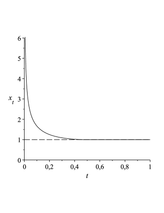
Figure 1. The unit ball for the $(t)$-norm in $\mathbb{R}^{2}$.

Let us mention that the solution to the equation $F_{\mu_{x}}(w)=0$ corresponds to an atom, that is, if the solution $w_{x}$ is of $F_{\mu_{x}}(w)=0$, the norm t is achieved either at an atom of $\mu_{x}^{\boxplus t}$ or at a point where the density of this measure is infinite. Atoms of the probability measure $\mu_{x}^{\boxplus 1/t}$ have been fully described in [5] by the formula

(14) $$\mu_{x}^{\boxplus 1/t}\left(\{a\}\right)=\max\left\{0,\frac{1}{t}\mu_{x}\left(\{ta\}\right)-\frac{1}{t}+1\right\}.$$

Let us record for further use that the above implies that when $t<\frac{1}{k}$ the measure $\mu_{x}^{\boxplus 1/t}$ is necessarily absolutely continuous with respect to the Lebesgue measure on $\mathbb{R}$.

3.5. The $(t)$-norm: continuity

This section contains a technical result for the continuity of the $(t)$-norm in $t$ and of the $\boxtimes$ operation. Proposition 3.8 is the main result here and it has independent interest in free probability. In the rest of this paper, we shall use a simpler incarnation of this result in the form of Corollary 3.9.

Proposition 3.7.

Assume that $\mu$ is a compactly supported probability measure on $[0,+\infty)$. Then the map $[1,+\infty)\ni t\mapsto[\mu^{\boxplus t}]\in(0,+\infty)$ is continuous, algebraic outside a bounded discrete subset of $(1,+\infty)$. Moreover,

(15) $$0<[\mu^{\boxplus t+\varepsilon}]-[\mu^{\boxplus t}]<t\left(\sqrt{\varepsilon\textrm{VAR}(\mu)}+\varepsilon\textrm{VAR}(\mu)\right),\quad t\geq 1,\varepsilon>0.$$

Proof.

As noted before, $[\mu^{\boxplus t}]$ is the largest positive number where either $F_{\mu^{\boxplus t}}$ is not analytic, or $F_{\mu^{\boxplus t}}$ takes the value zero. We shall use equations (10) in order to analyze this number. It follows easily that $F_{\mu^{\boxplus t}}$ is not analytic in $x_{0}$ if and only if $\omega_{t}$ is not analytic in $x_{0}$. This latter function is the right inverse of

$$H_{t}(w)=tw+(1-t)F_{\mu}(w)=w+(t-1)\int_{[0,+\infty)}s\,d\mu(s)+(1-t)\int_{[0,+\infty)}\frac{1}{s-w}\,d\rho(s),$$

according to the Nevanlinna representation of $F_{\mu}$.

One can see directly that for any $w$ in the interval of analyticity of $H_{t}$ included in $([\mu],+\infty)$, we have $H_{t}(w)>w$, $H_{t}^{\prime}(w)=1+(1-t)\int\frac{1}{(s-w)^{2}}\,d\rho(s).$ For simplicity, we shall denote $x_{t}$ the largest point in the real line in which $\omega_{t}$ is not analytic. Thus, $H_{t}$ maps the interval $[\max\{(H_{t}^{\prime})^{-1}(\{0\}),[\rho]\},+\infty)$ bijectively onto $[x_{t},+\infty)$. For $t>1$ large enough, it is clear that $[\max\{(H_{t}^{\prime})^{-1}(\{0\}),[\rho]\},+\infty)=[\max(H_{t}^{\prime})^{-1}(\{0\}),+\infty)$, and so the correspondence $t\mapsto\max(H_{t}^{\prime})^{-1}(\{0\})$ is clearly algebraic (in fact analytic). The relation $H_{t}(\omega_{t}(x))=x$ implies that $x_{t}=H_{t}(\max(H_{t}^{\prime})^{-1}(\{0\})),$ which is an analytic function. As $t$ decreases towards 1, it may happen (whenever $\lim_{w\downarrow[\rho]}\int\frac{1}{(s-w)^{2}}\,d\rho(s)<+\infty$) that $\max(H_{t}^{\prime})^{-1}(\{0\})$ either does not exist, or is no greater than $[\rho]$. We shall note that in this case there is a $t_{0}=1+\left(\lim_{w\downarrow[\rho]}\int\frac{1}{(s-w)^{2}}\,d\rho(s)\right)^{-1}$ so that the function $t\mapsto x_{t}$ is analytic on $(t_{0},+\infty)$ and extends continuously to $t_{0}$. On the interval $[1,t_{0}]$ we have, by the same relation $H_{t}(\omega_{t}(x))=x$,

$$x_{t}=H_{t}([\rho])=t[\rho]+(1-t)\lim_{w\downarrow[\rho]}F_{\mu}(w),$$

which is again an analytic (linear!) map of $t$. We note that $\lim_{w\downarrow[\rho]}F_{\mu}(w)$ must be finite as long as $\lim_{w\downarrow[\rho]}\int\frac{1}{(s-w)^{2}}\,d\rho(s)<+\infty$.

This has determined the analyticity of the correspondence between $t$ and the largest point of non-analyticity of $\omega_{t}$, and hence of $F_{\mu^{\boxplus t}}$. We have however remarked at the beginning of our proof that this point does not necessarily coincide with $[\mu^{\boxplus t}]$, and that moreover, the case in which it does not coincide corresponds to the case of an isolated atom of $\mu^{\boxplus t}$. Atoms of $\mu^{\boxplus t}$ have been however described in equation (14); it follows that the correspondence remains linear for $t$ in the interval $[1,(1-\mu(\{a\}))^{-1}]$. Moreover, when $t=(1-\mu(\{a\}))^{-1}$, we have $H_{t}^{\prime}(a)=t+(1-t)F_{\mu}^{\prime}(a)=t+(1-t)/\mu(\{a\})=(1-\mu(\{a\}))^{-1}+(1-(1-\mu(\{a\}))^{-1})/\mu(\{a\})=0$ (derivatives understood either in their proper sense, or in the Julia-Carathéodory sense), so at $t=(1-\mu(\{a\}))^{-1}$ we encounter a breach of analyticity of $\omega_{t}$ at the point $ta$.

This allows us to conclude that $t\mapsto[\mu^{\boxplus t}]$ has two possible regimes of evolution, either linear or according to $H_{t}(\max(H_{t}^{\prime})^{-1}(\{0\}))$, and the two regimes “glue” continuously. This guarantees continuity of $t\mapsto[\mu^{\boxplus t}]$ on $(0,+\infty)$. If the linear evolution occurs at all, then continuity at $t=1$ is obvious. If it does not, then we observe that $\lim_{t\to 1}\max(H_{t}^{\prime})^{-1}(\{0\})=[\rho]=[\mu]$, and moreover we can specify, by the Nevanlinna representation, that

$$0<\max(H_{t}^{\prime})^{-1}(\{0\})-[\mu]<\sqrt{(t-1)\rho(\mathbb{R})}=\sqrt{(t-1)\left(\int s^{2}\,d\mu(s)-\left[\int s\,d\mu(s)\right]^{2}\right)}.$$

Then

$$[\mu^{\boxplus t}]=H_{t}(\max(H_{t}^{\prime})^{-1}(\{0\}))=\max(H_{t}^{\prime})^{-1}(\{0\})+(t-1)\int s-\frac{1}{s-\max(H_{t}^{\prime})^{-1}(\{0\})}\,d\rho(s),$$

so it is enough to estimate $\left|(t-1)\int\frac{1}{s-\max(H_{t}^{\prime})^{-1}(\{0\})}\,d\rho(s)\right|.$ Recalling the equation determining $\max(H_{t}^{\prime})^{-1}(\{0\})$, namely $\int\frac{1}{(s-\max(H_{t}^{\prime})^{-1}(\{0\}))^{2}}\,d\rho(s)=\frac{1}{t-1}$, and noting that $\left(\int\frac{1}{s-\max(H_{t}^{\prime})^{-1}(\{0\})}\,d\rho(s)\right)^{2}<\rho(\mathbb{R})\int\frac{1}{(s-\max(H_{t}^{\prime})^{-1}(\{0\}))^{2}}\,d\rho(s)$, we get

$$\left((t-1)\int\frac{1}{s-\max(H_{t}^{\prime})^{-1}(\{0\})}\,d\rho(s)\right)^{2} < (t-1)^{2}\int\frac{\rho(\mathbb{R})}{(s-\max(H_{t}^{\prime})^{-1}(\{0\}))^{2}}\,d\rho(s)$$

$$= (t-1)\rho(\mathbb{R}).$$

We obtain

$$0<[\mu^{\boxplus t}]-[\mu]<\sqrt{(t-1)\rho(\mathbb{R})}+(t-1)\rho(\mathbb{R}).$$

This, together with the fact that the variance of $\mu^{\boxplus t}$ equals $t$ times the variance of $\mu$, guarantees that

$$0<[\mu^{\boxplus t+\varepsilon}]-[\mu^{\boxplus t}]<t(\sqrt{\varepsilon\rho(\mathbb{R})}+\varepsilon\rho(\mathbb{R})).$$

Since $\rho(\mathbb{R})=\textrm{VAR}(\mu)$, this concludes our proof. ∎

Note that, while the estimate provided by the above lemma is indeed optimal at $t=1$, it is not optimal throughout $(1,+\infty)$. However, it will serve our purposes. Also, it is worth mentioning that the correspondence $t\mapsto[\mu^{\boxplus t}]$ may fail to be analytic on $(1,+\infty)$ only due to a “phase transition” from a linear to an essentially inverse quadratic regime.

Next we address the problem of continuity for the upper bound of the support of the multiplicative free convolution of two probability distributions on the positive half-line. More precisely, assume that there is a topological space $X$ and a pair of functions $f,g\colon X\to(\mathcal{A}^{+},\varphi)$, where $\mathcal{A}^{+}$ denotes the set of positive elements in the non-commutative probability space $(\mathcal{A},\varphi)$. Assume that $f,g$ are weak* continuous (meaning that $X\ni\xi\mapsto\mu_{f(\xi)}$ is continuous from the topology of $X$ to the weak topology on the space of probability distributions compactly supported on $[0,+\infty)$, and the same for $g$), and in addition the maps $X\ni\xi\mapsto\|f(\xi)\|,X\ni\xi\mapsto\|g(\xi)\|$ are continuous. As noted before, $\|f(\xi)\|=[\mu_{f(\xi)}],$ and we shall use the two notations interchangeably.

It was noted before that $[\mu_{f(\xi)}]$ coincides with $\max\{x\in\mathbb{R}\colon G_{\mu_{f(\xi)}}\textrm{ not analytic in }x\}$. Equation (5) allows us to re-phrase this in terms of the moment generating function as

$$\frac{1}{[\mu_{f(\xi)}]}=\min\{x\in\mathbb{R}\colon\psi_{\mu_{f(\xi)}}\textrm{ not analytic in }x\}.$$

Let us recall that for any $\mu\neq\delta_{0}$ supported on the positive half-line, $\psi_{\mu}$ is strictly increasing on the interval $(-\infty,1/[\mu])$, so $\lim_{x\uparrow 1/[\mu]}\psi_{\mu}(x)$ exists in $(0,+\infty]$. We shall denote it by $\psi_{\mu}(1/[\mu])$. In particular, the inverse function $\psi^{-1}_{\mu}$ of $\psi_{\mu}$ is defined on $(\mu(\{0\})-1,\psi_{\mu}(1/[\mu])]$, monotonic, and takes values in $\left(-\infty,1/[\mu]\right]$. However, it is clear that $\psi_{\mu}^{-1}$ might have an analytic extension beyond $\psi_{\mu}(1/[\mu])$; indeed, that would correspond to the case when $(\psi_{\mu}^{-1})^{\prime}(\psi_{\mu}(1/[\mu]))=0$. Thus, we can give a description of $[\mu]$ in terms of $\psi_{\mu}^{-1}$:

$$\frac{1}{[\mu]}=\min\left\{\psi_{\mu}^{-1}(x)\colon(\psi_{\mu}^{-1})^{\prime}(r)>0\forall r<x,\psi_{\mu}^{-1}\textrm{ not analytic in }x\textrm{ or }(\psi_{\mu}^{-1})^{\prime}(x)=0\right\}.$$

(The case $x=+\infty$ is not excluded.)

The following proposition is concerned with the continuity of the correspondence $X\ni\xi\mapsto[\mu_{f(\xi)}\boxtimes\mu_{g(\xi)}]$ or, equivalently, the correspondence $X\ni\xi\mapsto\|f(\xi)g(\xi)\|$, where the sets $f(X)$ and $g(X)$ are assumed to be free with respect to $\varphi$. For mere convenience, we assume $X$ to be a metric space. We shall denote by $M_{f(\xi)}$ the largest positive number with the property that $\psi_{\mu_{f(\xi)}}^{-1}$ extends analytically to a complex neighbourhood of the interval $(\mu_{f(\xi)}(\{0\})-1,M_{f(\xi)}).$ We will assume that $\psi_{\mu_{f(\xi)}}^{-1}$ extends continuously as a real function to $M_{f(\xi)}$ and we will denote by $\tilde{\psi}_{\mu_{f(\xi)}}^{-1}$ the continuous extension

$$\tilde{\psi}_{\mu_{f(\xi)}}^{-1}(x)=\left\{\begin{array}[]{lcl}{\psi}_{\mu_{f(\xi)}}^{-1}(x)&\textrm{if}&x<M_{f(\xi)}\\ \displaystyle\lim_{r\uparrow M_{f(\xi)}}{\psi}_{\mu_{f(\xi)}}^{-1}(r)&\textrm{if}&x\geq M_{f(\xi)}\end{array}\right.$$

Proposition 3.8.

Let $X$ be a metric space, $(\mathcal{A},\varphi)$ a non-commutative probability space and $f,g\colon X\to(\mathcal{A}^{+}\setminus\{0\},\varphi)$ two norm-bounded functions that take values in free subalgebras of $\mathcal{A}$ satisfying the following conditions:

1. The correspondences $X\ni\xi\mapsto\mu_{f(\xi)},\mu_{g(\xi)}$ are weakly continuous;

2. The correspondences $X\ni\xi\mapsto\|f(\xi)\|,\|g(\xi)\|\in(0,+\infty)$ are continuous;

3. The correspondences $X\ni\xi\mapsto M_{f(\xi)},M_{g(\xi)}\in(0,+\infty]$ are continuous;

4. The correspondences $X\ni\xi\mapsto\tilde{\psi}_{\mu_{f(\xi)}}^{-1},\tilde{\psi}_{\mu_{g(\xi)}}^{-1}$ are continuous in the uniform norm, in the sense that for any $\xi_{0}\in X$,

   $$\lim_{\xi\to\xi_{0}}\sup_{r\in[0,+\infty]}|\tilde{\psi}_{\mu_{f(\xi)}}^{-1}(r)-\tilde{\psi}_{\mu_{f(\xi_{0})}}^{-1}(r)|=0.$$

5. If $\psi_{\mu_{f(\xi_{0})}}^{-1}$ is analytic on some complex neighborhood of $[0,r]$, then there exists a neighborhood $\mathcal{U}$ of $\xi_{0}$ and a complex neighborhood $V$ of $[0,r]$ so that $\psi_{\mu_{f(\xi)}}^{-1}$ is analytic on $V$ for all $\xi\in\mathcal{U}$. Same statement is required to hold for $g$.

Then the correspondence $X\ni\xi\mapsto[\mu_{f(\xi)}\boxtimes\mu_{g(\xi)}]\in(0,+\infty)$ is continuous.

Before starting the proof, we should mention that, as weak continuity for $f$ (condition (1)) is equivalent to continuity in the topology of the uniform convergence on compacts for $\psi_{\mu_{f(\xi)}}$, if $\{\xi_{n}\}_{n\in\mathbb{N}}\subseteq X$ converges to $\xi_{0}$ and $\psi_{\mu_{f(\xi_{n})}}^{-1},\psi_{\mu_{f(\xi_{0})}}^{-1}$ have a common domain, then $\psi_{\mu_{f(\xi_{n})}}^{-1}$ converges to $\psi_{\mu_{f(\xi_{0})}}^{-1}$ uniformly on compacts of the common domain. Condition (5) is devised in order to efficiently exploit this property. Condition (4) is a bit stronger than it appears: it says that if $\xi_{n}$ converges to $\xi$ in $X$ and $r_{n}\in[0,M_{f(\xi_{n})}]$ converges to $r\in[0,M_{f(\xi)}]$, then $\psi_{\mu_{f(\xi_{n})}}^{-1}(r_{n})$ converges to $\psi_{\mu_{f(\xi)}}^{-1}(r)$ as $n\to\infty$. Indeed, $|\psi_{\mu_{f(\xi)}}^{-1}(r)-\tilde{\psi}_{\mu_{f(\xi)}}^{-1}(r_{n})|\to 0$ as $n\to\infty$ by the continuity of $\tilde{\psi}_{\mu_{f(\xi)}}^{-1}$, and $|\tilde{\psi}_{\mu_{f(\xi)}}^{-1}(r_{n})-{\psi}_{\mu_{f(\xi_{n})}}^{-1}(r_{n})|\to 0$ as $n\to\infty$ by condition (4). In addition, our convention for doing arithmetics with infinity are $\infty+$ a real number $=\infty$, and $\infty-\infty=0$, so that the sets $\{x:\tilde{\psi}_{\mu_{f(\xi)}}^{-1}(x)=+\infty\}$ and $\{x:\tilde{\psi}_{\mu_{f(\xi_{n})}}^{-1}(x)=+\infty\}$ must coincide when $n$ is large enough.

Proof.

The statement of the proposition is local in nature: thus, let us choose $\xi_{0}\in X$ and an arbitrary sequence $\{\xi_{n}\}_{n\in\mathbb{N}}\subseteq X$ converging to $\xi_{0}$. It should be recorded that condition (1) and the weak continuity result of Bercovici and Voiculescu [10] for free multiplicative convolution implies that $\liminf_{n\to\infty}[\mu_{f(\xi_{n})}\boxtimes\mu_{g(\xi_{n})}]\geq[\mu_{f(\xi_{0})}\boxtimes\mu_{g(\xi_{0})}]$ (we might “lose,” but not “gain” support when passing to weak limit). We shall prove that $\lim_{n\to\infty}[\mu_{f(\xi_{n})}\boxtimes\mu_{g(\xi_{n})}]=[\mu_{f(\xi_{0})}\boxtimes\mu_{g(\xi_{0})}].$ In order to do that, we shall use (6), the $S$-transform property of Voiculescu. This translates, in terms of the moment-generating function, in

$$\psi_{\mu_{f(\xi)}\boxtimes\mu_{g(\xi)}}^{-1}(z)=\frac{1+z}{z}\psi_{\mu_{f(\xi)}}^{-1}(z)\psi_{\mu_{g(\xi)}}^{-1}(z).$$

This relation holds for $z$ in the interval bounded below by $\max\left\{\mu_{f(\xi)}(\{0\}),\mu_{g(\xi)}(\{0\})\right\}-1$ and above by the minimum between the domains of $\psi_{\mu_{f(\xi)}}^{-1}$ and $\psi_{\mu_{g(\xi)}}^{-1}$ viewed as inverses of the corresponding functions. However, there are many circumstances in which the above equality can be continued analytically (as complex functions) further along the positive axis. The maximum domain in $\mathbb{R}$ is the interval $(\max\left\{\mu_{f(\xi)}(\{0\}),\mu_{g(\xi)}(\{0\})\right\}-1,M_{\xi}]$, where $M_{\xi}$ is no smaller than the least of the upper bounds $M_{f(\xi)},M_{g(\xi)}$ of the domains of $\psi_{\mu_{f(\xi)}}^{-1}$ and $\psi_{\mu_{g(\xi)}}^{-1}$. In that case, $1/[\mu_{f(\xi)}\boxtimes\mu_{g(\xi)}]$ equals the either $\psi_{\mu_{f(\xi)}\boxtimes\mu_{g(\xi)}}^{-1}(M_{\xi})$ or $\psi_{\mu_{f(\xi)}\boxtimes\mu_{g(\xi)}}^{-1}(x_{\xi})$, where $x_{\xi}$ is the smallest critical point of $\psi_{\mu_{f(\xi)}\boxtimes\mu_{g(\xi)}}^{-1}$, if existing.

For simplicity, we shall denote $a_{n}=\psi_{\mu_{f(\xi_{n})}}^{-1},b_{n}=\psi_{\mu_{g(\xi_{n})}}^{-1},c_{n}=\psi_{\mu_{f(\xi_{n})}\boxtimes\mu_{g(\xi_{n})}}^{-1}$, with the obvious changes when $n$ is replaced by $0$ or simply eliminated. We shall split the proof in two cases:
Case 1: There exists a point $x_{\xi_{0}}>0$ in the domain of $c_{0}$ so that $c_{0}^{\prime}(x_{\xi_{0}})=0$ as a complex function. Without loss of generality, we may assume that this point $x_{\xi_{0}}$ is the smallest satisfying this condition, so that $c_{0}(x_{\xi_{0}})=1/[\mu_{f(\xi_{0})}\boxtimes\mu_{g(\xi_{0})}]$ (and thus $c_{0}$ extends analytically on a complex neighborhood of $[0,x_{\xi_{0}}]$).

Thus, by the $S$-transform property, there is a neighborhood of $[0,x_{\xi_{0}})$ on which $a_{0}$ and $b_{0}$ extend analytically. Indeed, assume towards contradiction there exists a point $r\in(0,x_{\xi_{0}})$ so that, say, $a_{0}$ does not extend analytically to it.

Our hypothesis for Case 1 guarantees that $\psi_{\mu_{f(\xi_{0})}\boxtimes\mu_{g(\xi_{0})}}([0,1/[\mu_{f(\xi_{0})}\boxtimes\mu_{g(\xi_{0})}]])=[0,x_{\xi_{0}}]$ (bijective correspondence) and the only obstacle to the analytic extension of $\psi_{\mu_{f(\xi_{0})}\boxtimes\mu_{g(\xi_{0})}}$ to $1/[\mu_{f(\xi_{0})}\boxtimes\mu_{g(\xi_{0})}]$ is the zero derivative of $c_{0}$ in $x_{\xi_{0}}$. If we replace in the moment-generating function version of the $S$-transform equation (given above) the variable $z$ by $\psi_{\mu_{f(\xi_{0})}\boxtimes\mu_{g(\xi_{0})}}(z)$ we obtain

$$z\frac{\psi_{\mu_{f(\xi_{0})}\boxtimes\mu_{g(\xi_{0})}}(z)}{\psi_{\mu_{f(\xi_{0})}\boxtimes\mu_{g(\xi_{0})}}(z)+1}=a_{0}(\psi_{\mu_{f(\xi_{0})}\boxtimes\mu_{g(\xi_{0})}}(z))b_{0}(\psi_{\mu_{f(\xi_{0})}\boxtimes\mu_{g(\xi_{0})}}(z)).$$

Denote for convenience $\omega_{1}=a_{0}\circ\psi_{\mu_{f(\xi_{0})}\boxtimes\mu_{g(\xi_{0})}},\omega_{2}=b_{0}\circ\psi_{\mu_{f(\xi_{0})}\boxtimes\mu_{g(\xi_{0})}}.$ It has been shown in [13] that $\omega_{j}$ extend analytically to $\mathbb{C}\setminus[0,+\infty)$, preserve $\mathbb{C}^{+}$ and increase the argument of the variable ($\arg\omega_{j}(z)\geq\arg z,$ $z\in\mathbb{C}^{+})$, and in [3] that their restriction to the upper half-plane extends continuously to $\mathbb{R}$. In particular, $a_{0},b_{0}$ extend continuously to $[0,x_{\xi_{0}}]$. Moreover, since $\psi_{\mu_{f(\xi_{0})}\boxtimes\mu_{g(\xi_{0})}}$ is real on $[0,1/[{\mu_{f(\xi_{0})}\boxtimes\mu_{g(\xi_{0})}}]],$ $\omega_{1},\omega_{2}$ must also be real on this same interval (see also [3]), and thus $a_{0},b_{0}$ are continuous real functions on $[0,x_{\xi_{0}}]$. A direct application of the Schwarz reflection principle guarantees that $a_{0},b_{0}$ extend analytically to a neighborhood of $[0,x_{\xi_{0}})$ in $\mathbb{C}$, as claimed. It should be noted in addition that, as $\omega_{j}$ preserve half-planes (see [13]), both $\omega_{j}$ are analytic on $[0,1/[\mu_{f(\xi_{0})}\boxtimes\mu_{g(\xi_{0})}])$, and so $a_{0}^{\prime}(r),b_{0}^{\prime}(r)>0$ for all $r\in[0,x_{\xi_{0}})$.

The analytic extension of $c_{0}$ around $x_{\xi_{0}}$ together with the fact that $c^{\prime}_{0}(x_{\xi_{0}})=0$ guarantees that there exists an $n>0$ so that $z\mapsto(\psi_{\mu_{f(\xi_{0})}\boxtimes\mu_{g(\xi_{0})}}(z)-\psi_{\mu_{f(\xi_{0})}\boxtimes\mu_{g(\xi_{0})}}(1/[\mu_{f(\xi_{0})}\boxtimes\mu_{g(\xi_{0})}]))^{n}$ is analytic in a neighborhood of $1/[\mu_{f(\xi_{0})}\boxtimes\mu_{g(\xi_{0})}]$. We shall denote $\mathcal{S}$ the Riemann surface determined by the corresponding $n^{\rm th}$ root. We shall argue that, with the above notations, $\omega_{1}$ and $\omega_{2}$ extend analytically to a piece of $\mathcal{S}$ which projects onto a neighborhood of $1/[\mu_{f(\xi_{0})}\boxtimes\mu_{g(\xi_{0})}]$ (of course, excluding $1/[\mu_{f(\xi_{0})}\boxtimes\mu_{g(\xi_{0})}]$). We shall do this at first under the additional assumption that $\psi_{\mu_{f(\xi_{0})}}$ and $\psi_{\mu_{g(\xi_{0})}}$ do not share any critical values. Indeed, let us follow $\psi_{\mu_{f(\xi_{0})}\boxtimes\mu_{g(\xi_{0})}}=\psi_{\mu_{f(\xi_{0})}}\circ\omega_{1}$ along an arbitrary path $p$ in $\mathcal{S}$ starting in the upper half-plane close enough to $1/[\mu_{f(\xi_{0})}\boxtimes\mu_{g(\xi_{0})}]$. Since $\arg\psi_{\mu_{f(\xi_{0})}}(w)\geq\arg w$ for $w$ in the upper half-plane, $\psi_{\mu_{f(\xi_{0})}\boxtimes\mu_{g(\xi_{0})}}(z)$ will stay in the upper half-plane as long as $\omega_{1}(z)$ does. Thus, we can then write $\omega_{1}(z)=\psi_{\mu_{f(\xi_{0})}}^{-1}(\psi_{\mu_{f(\xi_{0})}\boxtimes\mu_{g(\xi_{0})}}(z))$ whenever $\omega_{1}(z)$ is still in $\mathbb{C}^{+}$ as $z$ runs through $p$. The only obstacle to the analytic extension of $\omega_{1}$ through a $z_{k}$ is a zero derivative of $\psi_{\mu_{f(\xi_{0})}}$ in the point $\omega_{1}(z_{k})\in\mathbb{C}^{+}$. Then $\psi_{\mu_{f(\xi_{0})}}^{\prime}(\omega_{1}(z_{k}))\omega_{1}^{\prime}(z_{k})=\psi_{\mu_{f(\xi_{0})}\boxtimes\mu_{g(\xi_{0})}}^{\prime}(z_{k})$. As without loss of generality $\psi_{\mu_{f(\xi_{0})}\boxtimes\mu_{g(\xi_{0})}}^{\prime}(z_{k})\neq 0$, it follows that $\omega^{\prime}_{1}$ has infinite limit in $z_{k}.$ Since also $\psi_{\mu_{g(\xi_{0})}}^{\prime}(\omega_{2}(z_{k}))\omega_{2}^{\prime}(z_{k})=\psi_{\mu_{f(\xi_{0})}\boxtimes\mu_{g(\xi_{0})}}^{\prime}(z_{k})$, it follows from the $S$-transform equation and analytic continuation that necessarily $\omega_{2}^{\prime}(z_{k})$ is infinite, and moreover, the zeros of $\psi_{\mu_{f(\xi_{0})}}^{\prime}$ and $\psi_{\mu_{g(\xi_{0})}}^{\prime}$ in $\omega_{1}(z_{k})$ and $\omega_{2}(z_{k})$, respectively, must be of the same order. But since $\psi_{\mu_{f(\xi_{0})}\boxtimes\mu_{g(\xi_{0})}}=\psi_{\mu_{f(\xi_{0})}}\circ\omega_{1}=\psi_{\mu_{g(\xi_{0})}}\circ\omega_{2}$, we conclude that $\psi_{\mu_{f(\xi_{0})}}$ and $\psi_{\mu_{g(\xi_{0})}}$ share the critical value $\psi_{\mu_{f(\xi_{0})}\boxtimes\mu_{g(\xi_{0})}}(z_{k}),$ contradicting our hypothesis. (For the origins of this idea, see [35].)

Thus, under the additional hypothesis regarding critical values, we have shown that $\omega_{1}$ and $\omega_{2}$ extend to a simply connected domain $D$ of $\mathcal{S}$ which they map onto $V\setminus[\omega_{1}(1/[\mu_{f(\xi_{0})}\boxtimes\mu_{g(\xi_{0})}]),+\infty)$ and $V^{\prime}\setminus[\omega_{2}(1/[\mu_{f(\xi_{0})}\boxtimes\mu_{g(\xi_{0})}]),+\infty)$, respectively. Here $V$ and $V^{\prime}$ are complex neighborhoods of $\omega_{1}(1/[\mu_{f(\xi_{0})}\boxtimes\mu_{g(\xi_{0})}])$ and $\omega_{2}(1/[\mu_{f(\xi_{0})}\boxtimes\mu_{g(\xi_{0})}])$, respectively. Moreover, these extensions still satisfy the relations $\psi_{\mu_{f(\xi_{0})}\boxtimes\mu_{g(\xi_{0})}}=\psi_{\mu_{f(\xi_{0})}}\circ\omega_{1}=\psi_{\mu_{g(\xi_{0})}}\circ\omega_{2}$. Since $\psi_{\mu_{f(\xi_{0})}\boxtimes\mu_{g(\xi_{0})}}$ extends analytically to all of $\overline{D}$, we use the fact that the moment generating functions increase arguments to conclude that $\psi_{\mu_{f(\xi_{0})}}$ and $\psi_{\mu_{g(\xi_{0})}}$ must extend analytically to some interval $(a_{0}(x_{\xi_{0}}),a_{0}(x_{\xi_{0}})+\varepsilon)$ and $(b_{0}(x_{\xi_{0}}),b_{0}(x_{\xi_{0}})+\varepsilon)$, respectively, and thus $a_{0}$ and $b_{0}$ must themselves extend analytically (and bijectively!) to some complex neighborhood of $[0,x_{\xi_{0}}]$.

We have proved our claim under the additional assumption that $\psi_{\mu_{f(\xi_{0})}}$ and $\psi_{\mu_{g(\xi_{0})}}$ do not share any critical values. To complete the proof of our claim that $a_{0},b_{0}$ extend to some complex neighborhood of $[0,x_{\xi_{0}}]$ regardless of this condition being fulfilled, we only need to observe that a translation of a measure $\mu$ by a real number $k$ from the point of view of $w\mapsto\psi_{\mu}(w)=w^{-1}G_{\mu}(w^{-1})-1$ into $w\mapsto w^{-1}G_{\mu}(w^{-1}-k)-1$. Then $[w^{-1}G_{\mu}(w^{-1}-k)-1]^{\prime}=-w^{-2}G_{\mu}(w^{-1}-k)-w^{-3}G_{\mu}^{\prime}(w^{-1}-k)$. Thus, critical values change continuously in $k$. Since there can be at most countable critical values, we conclude that there exists a sequence $k_{m}$ tending to zero so that the moment generating functions of the translates of ${\mu_{f(\xi_{0})}}$ by $k_{m}$ and $\psi_{\mu_{g(\xi_{0})}}$ have no common critical values. Passing to the limit as $k_{m}\to 0$ provides the required answer.

But now the result under the assumption of Case 1 is proved; by part (5) of our Proposition there exists a neighborhood $V$ of $[0,x_{\xi_{0}}]$ on which $a_{n}$ and $b_{n}$ extend analytically, and by part (1) they converge to $a_{0}$ and $b_{0}$, respectively. By the $S$-transform property, $c_{n}\to c_{0}$ on $V$ as $n\to\infty$, so there are points $d_{n}\in(0,+\infty)$ so that $c_{n}^{\prime}(d_{n})=0$ and $\lim_{n\to\infty}d_{n}=x_{\xi_{0}}$. So $c_{n}(x_{\xi_{n}})=\lim_{k\to\infty}1/[\mu_{f(\xi_{n_{k}})}\boxtimes\mu_{g(\xi_{n_{k}})}]=1/[\mu_{f(\xi_{0})}\boxtimes\mu_{g(\xi_{0})}]=c_{0}(x_{\xi_{0}})$, as claimed.

Case 2: For any $x>0$ in the domain of $c_{0}$, we have $c_{0}^{\prime}(x)>0$. If we denote as before $M_{\xi_{0}}$ to be the upper bound of the domain of $c_{0}$, then $c_{0}(M_{\xi_{0}}):=\lim_{x\uparrow M_{\xi_{0}}}c_{0}(x)$ exists, belongs to $(0,+\infty)$ (although $M_{\xi_{0}}$ might be equal to $+\infty$) and equals $1/[\mu_{f(\xi_{0})}\boxtimes\mu_{g(\xi_{0})}]$. By the $S$-transform equation, it follows that at least one of $a_{0}$, $b_{0}$ must have $M_{\xi_{0}}$ as upper bound of the domain of analyticity. Without loss of generality, assume that $M_{\xi_{0}}=M_{f(\xi_{0})}$ is the upper bound for the domain of analyticity of $a_{0}$. Condition (3) implies that $M_{f(\xi_{n})}\to M_{f(\xi_{0})}$ as $n\to\infty$. As the same condition holds for $g$, we easily conclude that $\lim_{n\to\infty}\min\{M_{f(\xi_{n})},M_{g(\xi_{n})}\}=M_{\xi_{0}}$ (limits considered in $[0,+\infty]$). If there is an $n_{0}\in\mathbb{N}$ so that $c_{n}$ has no critical point in $(0,\min\{M_{f(\xi_{n})},M_{g(\xi_{n})}\})$ for any $n\geq n_{0}$, then condition (4) and the $S$-transform property allow us to conclude. Assume that for infinitely many $n$ the function $c_{n}$ has a critical point in $(0,\min\{M_{f(\xi_{n})},M_{g(\xi_{n})}\})$; call the smallest of them $\zeta_{n}$. Then we know that $c_{n}(\zeta_{n})=1/[\mu_{f(\xi_{n})}\boxtimes\mu_{g(\xi_{n})}]$. Since $a_{0},b_{0}$ are analytic on some complex neighborhood of $[0,M_{\xi_{0}})$, condition (5) tells us that for any $s\in[0,M_{\xi_{0}})$ there exists a neighborhood $V_{s}$ of $[0,s]$ in $\mathbb{C}$ so that, from a certain $n$ on, all $a_{n},b_{n}$ have an analytic extension to $V_{s}$. If there is a subsequence $\{\zeta_{n_{k}}\}_{k}$ which converges to a point $r<M_{\xi_{0}}$, then $c_{n_{k}}$ converges to $c_{0}$ uniformly on compacts of $V_{r}$ by condition (1) and thus $r$ is a critical point of $c_{0}$, contradicting the assumption of Case 2. The case when $\zeta_{n}$ converges to $M_{\xi_{0}}$ as $n\to\infty$ is covered by condition (4): indeed, this condition implies that $c_{n}(\zeta_{n})=\frac{1+\zeta_{n}}{\zeta_{n}}a_{n}(\zeta_{n})b_{n}(\zeta_{n})\to\frac{1+M_{\xi_{0}}}{M_{\xi_{0}}}a_{0}(M_{\xi_{0}})b_{0}(M_{\xi_{0}})=c_{0}(M_{\xi_{0}})$ as $n\to\infty$. (Here we use the obvious convention $\frac{1+\infty}{\infty}=1.)$ This concludes our proof. ∎

We would like to emphasize that some of the conditions of the above proposition can be weakened or replaced with conditions of a different nature: we use this set of conditions simply because it covers a conveniently large family of distributions for our purposes.

Corollary 3.9.

If $\mu$ is a fixed compactly supported probability measure on $[0,+\infty)$, $a=(a_{1},\dots,a_{m})\in[0,+\infty)^{m}\setminus\{(0,\dots,0)\}$, $t=(t_{1},\dots,t_{m})\in(0,1)^{m}\cap\Delta_{m}$ (so $(t_{1},\dots,t_{m})$ satisfy $\sum_{j=1}^{m}t_{j}=1$), and $\nu(a,t)=\sum_{j=1}^{m}t_{j}\delta_{a_{j}}$, then the correspondence $([0,+\infty)^{m}\setminus\{(0,\dots,0)\})\times\Delta_{m}\ni(a,t)\mapsto[\mu\boxtimes\nu(a,t)]$ is continuous.

Proof.

We shall apply the previous proposition, with the identifications $X=([0,+\infty)^{m}\setminus\{(0,\dots,0)\})\times\Delta_{m}$, $f$ the constant function taking value $\mu$, and $g(a,t)=\nu(a,t)=\sum_{j=1}^{m}t_{j}\delta_{a_{j}}$. One checks that $f$ satisfies all conditions from the proposition above.The weak continuity of $g$ is equally clear, as is the continuity of the correspondence $(a,t)\mapsto[\nu(a,t)].$ Observing that $\psi_{\nu(a,t)}$ maps $(-\infty,1/\max\{a_{1},\dots,a_{m}\})$ monotonically and bijectively into $\left(\left[\sum_{j\colon a_{j}=0}t_{j}\right]-1,+\infty\right)$ assures us that the upper bound of the domain of $\psi_{\nu(a,t)}^{-1}$ is constantly equal to infinity, and hence continuous, and moreover, $\psi_{\nu(a,t)}^{-1}$ maps plus infinity into $1/[\nu(a,t)]$, guaranteeing the continuity of $\psi_{\nu(a,t)}^{-1}(M_{g(a,t)})$, and hence the verification of conditions (3) and (4). Condition (5) is verified by the constant function $f$. For $g$ one only needs to recall the observations following equation (6) to note that indeed, given any compact subset of $X$, there is a complex neighbourhood of $[0,+\infty)$ on which $\psi_{\nu(a,t)}^{-1}$ is analytic for all $(a,t)$ in the given compact set. Thus, a stronger version of condition (5) is satisfied by $g$. Applying the above proposition allows us to conclude. ∎

4. Almost sure convergence of norms of random matrices

Let GUE be the Gaussian Unitary Ensemble, i.e. the probability measure on $\mathcal{M}_{n}(\mathbb{C})$ with support on self-adjoint matrices and density proportional to $\exp(-n/2\operatorname{Tr}(A^{2}))\mathrm{d}A$. The following theorem was obtained in the seminal paper [23] by Haagerup and Thorbjørnsen:

Theorem 4.1.

Let $X_{n},Y_{n}$ be two i.i.d GUE random variables on $\mathcal{M}_{n}(\mathbb{C})$ and $P$ be a non-commutative polynomial in two variables. Then, almost surely as $n\to\infty$,

$$\left\|P(X_{n},Y_{n})\right\|_{\infty}\to\left\|P(x,y)\right\|$$

where $x,y$ are free semi-circular elements in a finite von Neumann algebra.

The aim of this section is to build on Theorem 4.1, and extend it to some specific non-commutative monomials of random matrices with prescribed spectra.

We recall that if $X$ is an $n$-dimensional self-adjoint matrix, its eigenvalue counting measure is $n^{-1}\sum_{i=1}^{n}\delta_{\lambda_{i}}$ where $\lambda_{i}$ are the eigenvalues of $X$. For any probability measure $\mu$ on the real line, its distribution function is defined as $f_{\mu}:t\mapsto\mu((-\infty,t])$.

For the purposes of this section, we will say that a sequence of distribution functions $f_{n}$ tends to a distribution function $f$ iff for all $\varepsilon>0$, there exists an $n_{0}$ such that for all $n\geqslant n_{0}$,

(16) $$\forall t\in\mathbb{R},\quad f(t-\varepsilon)-\varepsilon\leqslant f_{n}(t)\leqslant f(t+\varepsilon)+\varepsilon$$

Theorem 4.2.

Let $A_{n},B_{n}$ be independent positive self-adjoint random matrices in $\mathcal{M}_{n}(\mathbb{C})$, such that at least one of $A_{n}$ or $B_{n}$ has a distribution invariant under unitary conjugation. Let $f_{n}$ be the distribution function of $A_{n}$ and $g_{n}$ be the distribution function of $B_{n}$. Assume that the (a priori random) distribution functions $f_{n},g_{n}$ converge almost surely respectively to $f,g$ which are distribution functions of two self-adjoint, bounded and freely independent random variables $x$ and $y$. Assume also that the operator norm of $A_{n}$ (resp. $B_{n}$) converges to the operator norm of $x$ (resp. $y$).

Then, almost surely as $n\to\infty$,

$$||A_{n}B_{n}||\to||xy||.$$

Similar results have been obtained recently by C. Male [25]. However, our results do not clearly follow from his. We also believe that the above theorem could be proved directly with determinantal processes methods, see e.g. [21, 26], at least in the case where one of the operators is a projection.

Note also that 6 months after the first version of this paper was completed, one author and C. Male used one key ingredient introduced in the proof below to prove a substantial extension of Theorem 4.1 in the unitary case, see [17]. The more recent main result of [17], even though quite general, does not imply directly Theorem 4.2 because our assumptions on the spectrum of $A_{n},B_{n}$ are not as restrictive as in [17].

Proof of Theorem 4.2.

Without loss of generality, we can assume that both $A_{n}$ and $B_{n}$ have distributions which are invariant under unitary conjugation (indeed, replacing the pair $(A_{n},B_{n})$ by $(V_{n}A_{n}V_{n}^{*},V_{n}B_{n}V_{n}^{*})$ where $V_{n}$ is a Haar distributed random state independent from $(A_{n},B_{n})$ does not change the hypotheses nor $||A_{n}B_{n}||$, but enforces unitary invariance on both $A_{n}$ and $B_{n}$.

The main idea is to adapt Theorem 4.1 to our case by showing that in the case where $P$ of Theorem 4.1 is of the form $P_{1}(x)P_{2}(y)$, it extends to the situation where $P_{1},P_{2}$ are any nondecreasing bounded functions.

In this proof we consider a pair $X_{n},Y_{n}\in\mathcal{M}_{n}(\mathbb{C})$ of i.i.d GUE random matrices and we split our proof into three steps. In the first two steps, we show how we can replace in Theorem 4.1 polynomials by real, non-decreasing, càdlàg, non-negative and bounded functions. In the third step, we show how, via functional calculus, we can modify the pair $(X_{n},Y_{n})$ into a pair that has the same distribution as $(A_{n},B_{n})$.

Step I. First, we prove that if $P$ is any real positive polynomial and $S_{0}$ is a distribution function (real, non-decreasing, càdlàg and positive), then, for all $\varepsilon>0$, for a fixed small enough neighborhood $\mathcal{V}$ of $S_{0}$, almost surely, there exists $n_{0}\in\mathbb{N}$ such that, for all $n\geqslant n_{0}$ and for all $S\in\mathcal{V}$,

(17) $$|\left\|P(X_{n})S(Y_{n})P(X_{n})\right\|_{\infty}-\left\|P(x)S(y)P(x)\right\||<\varepsilon,$$

were $x,y$ are free semicircular elements in a $\mathrm{II}_{1}$ factor.

For $\varepsilon>0$, we introduce the functions $S^{+}_{0}(x)=S_{0}(x+\varepsilon)+\varepsilon$ and $S^{+}_{0}(x)=S_{0}(x-\varepsilon)-\varepsilon$. Clearly, we have $S^{-}_{0}<S_{0}<S^{+}_{0}$. Moreover, since the neighborhood $\mathcal{V}$ of $S_{0}$ can be chosen as small as we need to, we can choose it in such a way that for all $S\in\mathcal{V}$, the jumping points of $S$ are at distance at most $\varepsilon/100$ from the jumping points of $S_{0}$. By Stone-Weierstrass theorem, there exist polynomials $Q^{\pm}$ such that, on the interval $[-3,3]$, for all $S\in\mathcal{V}$, $S^{-}_{0}<Q^{-}<S<Q^{+}<S^{+}_{0}$ (see Figure 2).

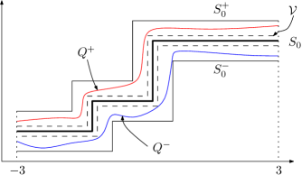
Figure 2. Bounding distribution functions uniformly by polynomials.

The fact that almost surely the eigenvalues of $X_{n}$ and $Y_{n}$ are included in $[-3,3]$ as $n\to\infty$ implies that almost surely, for all $S\in\mathcal{V}$ and for $n$ large enough, $S(Y_{n})<Q^{+}(Y_{n})$. Therefore, almost surely for $n$ large enough, $P(X_{n})S(Y_{n})P(X_{n})<P(X_{n})Q^{+}(Y_{n})P(X_{n})$ and thus, using positivity,

$$\left\|P(X_{n})S(Y_{n})P(X_{n})\right\|_{\infty}<\left\|P(X_{n})Q^{+}(Y_{n})P(X_{n})\right\|_{\infty}.$$

However, $P$ and $Q^{+}$ are polynomials, therefore we can use Theorem 4.1 to claim that $\left\|P(X_{n})Q^{+}(Y_{n})P(X_{n})\right\|_{\infty}\to\left\|P(x)Q^{+}(y)P(x)\right\|$. We have shown that, almost surely for $n$ large enough,

$$\limsup_{n\to\infty}\left\|P(X_{n})S(Y_{n})P(X_{n})\right\|_{\infty}\leqslant\left\|P(x)Q^{+}(y)P(x)\right\|.$$

In the von Neumann algebra generated by two free semicircular elements $x,y$, we have the inequality $P(x)Q^{+}(y)P(x)\leqslant P(x)S^{+}_{0}(y)P(x)$, therefore

$$\limsup_{n\to\infty}\left\|P(X_{n})S(Y_{n})P(X_{n})\right\|_{\infty}\leqslant\left\|P(x)S^{+}_{0}(y)P(x)\right\|.$$

Since this is true for all $\varepsilon>0$ and the norm is continuous according to Corollary 3.9, by letting $\varepsilon\to 0$ we get

$$\limsup_{n\to\infty}\left\|P(X_{n})S(Y_{n})P(X_{n})\right\|_{\infty}\leqslant\left\|P(x)S(y)P(x)\right\|.$$

A similar argument, using this time $Q^{-}$ and $S_{0}^{-}$ to bound from below elements $S\in\mathcal{V}$ proves the other inequality and completes the first step of the proof. Note however that the lower bound could have been obtained without using Theorem 4.1; indeed, one can use Voiculescu’s result for the convergence of empirical spectral distributions of random matrices to conclude.

Step II. The second part of our proof is to show that that one can replace the polynomial $P$ in equation (17) by another function $T$ chosen from a neighborhood $\mathcal{W}$ of a given distribution function $T_{0}$. First, note that in Step I, one can interchange the roles of the polynomial $P$ and the step function $S$ by using the $C^{*}$ algebra equality, $\left\|a\right\|^{2}=\left\|aa^{*}\right\|$. Hence, $\left\|S(X_{n})P(Y_{n})S(X_{n})\right\|_{\infty}$ converges to $\left\|S(x)P(y)S(x)\right\|$. Then, we employ the same technique as in Step I: we bound any element $T\in\mathcal{W}$ by fixed polynomials $P^{\pm}$ and we use Step I to conclude. Note that in the first two steps of the proof we have considered GUE matrices $X_{n}$ and $Y_{n}$.

Step III. In this final step, we consider our original sequence $(A_{n},B_{n})$ and show that our conclusion holds for it. For the purpose of its study, we introduce an auxiliary pair $(X_{n},Y_{n})$ of two i.i.d Gaussian ensembles. It is known that with probability one, all its eigenvalues have multiplicity one. So without loss of generality, we will assume that our instance of $(X_{n},Y_{n})$ does not have multiplicity in its eigenvalues. Similarly, we assume that the normalized eigenvalue counting function of $X_{n}$ and $Y_{n}$ converges towards the semi-circle and that their operator norm converges to 2. It is also possible to do so without loss of generality because of the well known convergence properties of the Gaussian unitary ensembles [23].

From this, it follows that there exists two non-decreasing càdlàg functions $f_{n}$, $g_{n}$ such that the eigenvalues of $f_{n}(X_{n})$ are the same as those of $A_{n}$ and the eigenvalues of $g_{n}(Y_{n})$ are the same as those of $B_{n}$.

The functions $f_{n}$ and $g_{n}$ are not unique and are random, but it follows from our hypotheses on the limiting distributions of $A_{n},B_{n}$ and our choice of $X_{n},Y_{n}$ that it is possible to make sure that $f_{n}$ and $g_{n}$ converge uniformly.

Let us denote by $a_{1}\geqslant\ldots\geqslant a_{n}$ the eigenvalues of $A_{n}$, $b_{1}\geqslant\ldots\geqslant b_{n}$ the eigenvalues of $B_{n}$, $x_{1}>\ldots>x_{n}$ the eigenvalues of $X_{n}$, and $y_{1}>\ldots>y_{n}$ the eigenvalues of $Y_{n}$ (note that we make a small abuse of notation for the sake of simplicity, and omit in the notation the dependence in $n$). It follows from the above that for all $i$, $f_{n}(x_{i})=a_{i}$ and $g_{n}(y_{i})=b_{i}$.

Next, let us introduce the decomposition $A_{n}=U_{a}\mathrm{diag}(a_{1},\ldots,a_{n})U_{a}^{*}$ and similarly for $B_{n},X_{n},Y_{n}$. It is known that it is possible to make a choice for $U_{a}$ (resp. $U_{b},U_{x},U_{y}$) that depends from $A_{n}$ (resp. $B_{n},X_{n},Y_{n}$) in a measurable way.

Let $\tilde{X}_{n}=U_{a}\mathrm{diag}(x_{1},\ldots,x_{n})U_{a}^{*}$ and $\tilde{Y}_{n}=U_{b}\mathrm{diag}(y_{1},\ldots,y_{n})U_{b}^{*}$.

The matrices $\tilde{X}_{n},\tilde{Y}_{n}$ are random matrices and they have the property that $f_{n}(\tilde{X}_{n})=A_{n}$ and $g_{n}(\tilde{Y}_{n})=B_{n}$. Besides, they are independent from each other. Finally, they both follow the GUE distribution because the latter is known to be determined by three criteria that are obviously satisfied in the construction of $\tilde{X}_{n},\tilde{Y}_{n}$, namely: (a) the distribution of its eigenvalues is the correct one, (b) its eigenvalues and its eigenvectors are independent, and (c) its eigenvectors are distributed according to the invariant measure.

We conclude the proof by an application of Step II to the matrices $\tilde{X}_{n},\tilde{Y}_{n}$ with the functions $f_{n},g_{n}$.

∎

5. Asymptotic behaviour of $K_{n,k,t}$

We now introduce the convex body $K_{k,t}\subset\Delta_{k}$ as follows:

(18) $$K_{k,t}:=\{\lambda\in\Delta_{k}\;|\;\forall a\in\Delta_{k},\langle\lambda,a\rangle\leqslant\left\|a\right\|_{(t)}\},$$

where $\langle\cdot,\cdot\rangle$ denotes the canonical scalar product in $\mathbb{R}^{k}$. We shall show in Theorem 6.4 that this set is intimately related to the $(t)$-norm: $K_{k,t}$ is the intersection of the dual ball of the $(t)$-norm with the probability simplex $\Delta_{k}$. Since it is defined by duality, $K_{k,t}$ is the intersection of the probability simplex with the half-spaces

$$H^{+}(a,t)=\{x\in\mathbb{R}^{k}\;|\;\langle x,a\rangle\leqslant\left\|a\right\|_{(t)}\}$$

for all directions $a\in\Delta_{k}$. Moreover, we shall show in Theorem 5.3 that every hyperplane $H(a,t)=\{x\in\mathbb{R}^{k}\;|\;\langle x,a\rangle=\left\|a\right\|_{(t)}\}$ is a supporting hyperplane for $K_{k,t}$.

5.1. A set of probability one and statement of the results

Let $(\Omega,\mathcal{F},\mathbb{P})$ be a probability space in which the sequence or random vector subspaces $(V_{n})_{n\geqslant 1}$ is defined. Since we assume that the elements of this sequence are independent, we may assume that $\Omega=\prod_{n\geqslant 1}\operatorname{Gr}_{N}(\mathbb{C}^{k}\otimes\mathbb{C}^{n})$ and $\mathbb{P}=\otimes_{n\geqslant 1}\mu_{n}$ where $\mu_{n}$ is the invariant measure on the Grassman manifold $\operatorname{Gr}_{N}(\mathbb{C}^{k}\otimes\mathbb{C}^{n})$. Let $P_{n}\in\mathcal{M}_{nk}(\mathbb{C})$ be the random orthogonal projection whose image is $V_{n}$. For two positive sequences $(a_{n})_{n}$ and $(b_{n})_{n}$, we write $a_{n}\ll b_{n}$ iff $a_{n}/b_{n}\to 0$ as $n\to\infty$.

Proposition 5.1.

Let $\nu_{n}$ be a sequence of integers satisfying $\nu_{n}\ll n$. Almost surely, the following holds true: for any self-adjoint matrix $A\in\mathcal{M}_{k}(\mathbb{C})$, the $\nu_{n}$-th largest eigenvalues of $P_{n}(A\otimes I_{n})P_{n}$ converges to $||a||_{(t)}$ where $a$ is the eigenvalue vector of $A$. This convergence is uniform on any compact set of $\mathcal{M}_{k}(\mathbb{C})_{sa}$.

Proof.

For any self-adjoint $A\in\mathcal{M}_{k}(\mathbb{C})$, the almost sure convergence follows from Theorem 4.2 and from Theorem 3.1.

Let $A_{l}$ be a countable family of self-adjoint matrices in $\mathcal{M}_{k}(\mathbb{C})$ and assume that their union is dense in the operator norm unit ball. By sigma-additivity, the property to be proved holds almost-surely simultaneously for all $A_{l}$’s.

This implies that the property holds for all $A$ almost-surely, as the $j$-th largest eigenvalue of a random matrix is a Lipschitz function for the operator norm on the space of matrices. ∎

The set on which the conclusion of the above proposition holds true will be denoted by $\Omega^{\prime}$ and we therefore have $\mathbb{P}(\Omega^{\prime})=1$. Technically, $\Omega^{\prime}$ depends on $\nu_{n}$ but in the proofs, we won’t need to keep track of this dependence as $\nu_{n}$ will be a fixed sequence.

The main result of our paper is the following characterization of the asymptotic behavior of the random set $K_{n,k,t}$. We show that this set converges, in a very strong sense, to the convex body $K_{k,t}$.

Theorem 5.2.

Almost surely, the following holds true:

• Let $\mathcal{O}$ be an open set in $\Delta_{k}$ containing $K_{k,t}$. Then, for $n$ large enough, $K_{n,k,t}\subset\mathcal{O}$.

• Let $\mathcal{K}$ be a compact set in the interior of $K_{k,t}$. Then, for $n$ large enough, $\mathcal{K}\subset K_{n,k,t}$.

The proof of this theorem goes according to the following non-standard scheme: the first inclusion follows a strategy developed in [19] and improves on it. This is the object of Theorem 5.4. Revisiting the strategy of proof of Theorem 5.4 gives rise to a result about eigenvectors of random matrices, as stated in Theorem 5.3 below, and in turn, Theorem 5.3 is needed to prove the second part of Theorem 5.2. This is the purpose of Theorem 5.10.

Note that all the statements above are of almost sure nature. At first sight this looks unnatural because there is no assumption on the probability space on which the family of random matrices indexed by the dimension is defined. The only assumptions are on the $n$-dimensional marginals. The fact that the results hold with probably one on any probability probability space having the appropriate marginals follows from arguments of Borel-Cantelli type.

Instead of stating a result of convergence almost surely, it is also possible, in the spirit of e.g. [2, Theorem 2.1.1], to write down a theorem of convergence in probability. The benefit of doing so is that one does not need to bother to realize all random matrices in a same probability space. Such a result actually follows from the above Theorem. We could have chosen such an approach, but we felt that the technical details of the proof would have been more involved (in our proof we intersect countably many probability one measurable subsets of an appropriate probability space). Note also that Anderson, Guionnet and Zeitouni also state results of almost sure convergence (see for example [2] Exercise 2.1.16). Similarly, in the original results by Haagerup and Thorbjørnsen, the convergence results are of almost sure nature.

A byproduct of the first part of the above theorem, and a necessary step towards its second part is the following result, of independent interest in random matrix theory:

Theorem 5.3.

Consider a matrix $A=\operatorname{diag}(a)$ whose eigenvalue vector is $a\in\mathbb{R}^{k}$ and let $\nu_{n}$ be a sequence of integers satisfying $\nu_{n}\ll n$. We assume that all eigenvalues of $A$ are simple.

Let $x^{(n)}$ be the unital eigenvector corresponding to the $\nu_{n}$-th largest eigenvalue of $P_{n}(A\otimes I_{n})P_{n}$, which admits a singular value decomposition

$$x^{(n)}=\sum_{i=1}^{k}\sqrt{\lambda_{i}^{(n)}}e_{i}^{(n)}\otimes f_{i}^{(n)}.$$

Then, almost surely, for each $i=1,2,\ldots,k$, $e_{i}^{(n)}$ converges to the eigenvector corresponding to the $i$-th largest eigenvalue of $A$ (modulo a phase change). Moreover, if $\lambda$ is the exposed point of $K_{k,t}$ such that the supporting hyperplane is defined by the direction $a$, then, almost surely

$$\lim_{n\to\infty}\lambda^{(n)}=\lambda.$$

This theorem has its own interest from the random matrix point of view. Indeed it can be seen as a law of large numbers for the $\mathcal{U}(k)/\mathcal{U}(1)^{k}$ and the $\mathbb{R}^{k}$ components of the singular value decomposition of the eigenvectors. Even though many laws of large numbers have been obtained for eigenvalues, not much is known about the structure of eigenvectors (except [27], [8] and references therein).

5.2. Upper bound

The first part of Theorem 5.2 is the following result:

Theorem 5.4.

Let $\mathcal{O}$ be an open set in $\Delta_{k}$ containing $K_{k,t}$. Then almost surely, for $n$ large enough, $K_{n,k,t}\subset\mathcal{O}$.

This result provides almost surely an upper bound for the set $K_{n,k,t}$. The proof of this theorem relies on Theorem 4.2, and on two lemmas, that are adapted from [19] and which we state and prove below.

Lemma 5.5.

Let $Q\in\mathcal{M}_{n}(\mathbb{C})$ be a self-adjoint projection and $R\in\mathcal{M}_{n}(\mathbb{C})$ be a self-adjoint element. Then

(19) $$\left\|QRQ\right\|_{\infty}=\max_{x\in\operatorname{Im}Q}\operatorname{Tr}(P_{x}R),$$

where $P_{x}$ denotes the orthogonal projection on the one-dimensional space $\mathbb{C}x$.

For two matrices $A,B\in\mathcal{M}_{k}(\mathbb{C})$, we write $A\sim B$ if there exists a unitary operator $U\in\mathcal{U}(k)$ such that $A=UBU^{*}$. For a vector $x\in\mathbb{C}^{k}\otimes\mathbb{C}^{n}$ with Schmidt coefficients $\lambda_{1}\geqslant\lambda_{2}\geqslant\cdots\geqslant\lambda_{k}\geqslant 0$, and an element $a\in\Delta_{k}^{\downarrow}$, we introduce the notation

$$s^{a}(x)=a_{1}\lambda_{1}+\ldots+a_{k}\lambda_{k}=\langle a,\lambda\rangle.$$

Similarly, for a matrix $A\in\mathcal{M}_{k}(\mathbb{C})$, we introduce the notation

$$s^{A}(x):=\operatorname{Tr}(P_{x}\cdot A\otimes\operatorname{I}_{n})=\operatorname{Tr}(\operatorname{Tr}_{n}P_{x}\cdot A),$$

where $\operatorname{Tr}_{n}=\operatorname{id}_{k}\otimes\operatorname{Tr}$ is the non-normalized conditional expectation $\mathcal{M}_{nk}(\mathbb{C})\to\mathcal{M}_{k}(\mathbb{C})$.

Lemma 5.6.

Let $A$ be a self-adjoint matrix with ordered eigenvalue vector $a\in\Delta_{k}^{\downarrow}$. For each $x\in\mathbb{C}^{k}\otimes\mathbb{C}^{n}$, the following holds true:

$$s^{a}(x)=\max_{A^{\prime}\sim A}s^{A^{\prime}}(x).$$

Proof.

For two matrices $A,B\in\mathcal{M}_{k}(\mathbb{C})$ with respective eigenvalues $\mu_{1}\geqslant\ldots\geqslant\mu_{k}\geqslant 0$ and $\lambda_{1}\geqslant\ldots\geqslant\lambda_{k}\geqslant 0$, it follows from the min-max theorem that

$$\sum_{i}\lambda_{i}\mu_{i}=\max_{A^{\prime}\sim A}\operatorname{Tr}(A^{\prime}B).$$

Letting $B=\operatorname{Tr}_{n}P_{x}$, the above observation implies:

(20) $$s^{a}(x)=\max_{U\in\mathcal{U}(k)}\operatorname{Tr}(UAU^{*}\operatorname{Tr}_{n}P_{x})=\max_{A^{\prime}\sim A}\operatorname{Tr}(A^{\prime}\operatorname{Tr}_{n}P_{x}).$$

The conditional expectation property of the partial trace implies that

(21) $$s^{a}(x)=\max_{A^{\prime}\sim A}\operatorname{Tr}(P_{x}\cdot A^{\prime}\otimes\operatorname{I}_{n})=\max_{A^{\prime}\sim A}s^{A^{\prime}}(x).$$

∎

Since $k$ is a fixed parameter of our model, in order to compute the maximum in Lemma 5.5 over the unitary orbit indexed by $\mathcal{U}(k)$, we can pick a finite but large enough number of elements of the corresponding orbit to obtain a good approximation of the maximum:

Lemma 5.7.

For a fixed self-adjoint matrix $A\in\mathcal{M}_{k}(\mathbb{C})$ with eigenvalue vector $a\in\mathbb{R}^{k}$ and for all $\varepsilon>0$, there exist a finite number of matrices $B_{1},\ldots,B_{l}$ self-adjoint and conjugated to $A$, such that, for all $x\in\mathbb{C}^{nk}$,

(22) $$\max_{i=1}^{l}\operatorname{Tr}(P_{x}\cdot B_{i}\otimes\operatorname{I}_{n})\leqslant s^{a}(x)\leqslant\max_{i=1}^{l}\operatorname{Tr}(P_{x}\cdot B_{i}\otimes\operatorname{I}_{n})+\varepsilon.$$

Proof.

We only need to prove the second inequality, the first one being a direct consequence of Lemma 5.6. Since the orbit under unitary conjugation of a self-adjoint matrix $A$ is compact for the metric $d(B,B^{\prime})=\left\|B-B^{\prime}\right\|_{\infty}$, for all $\varepsilon>0$ there exists a covering of the orbit by a finite number of balls of radius $\varepsilon$ centered in $B_{1},B_{2},\ldots,B_{l}$. Fix some $x\in\mathbb{C}^{nk}$ and consider the element $B$ in the orbit of $A$ for which the maximum in the definition of $s^{a}(x)$ is attained. The matrix $B$ is inside some ball centered at $B_{i}$ and we have

(23) $$\begin{split}\operatorname{Tr}(P_{x}\cdot B\otimes\operatorname{I}_{n})&\leqslant\operatorname{Tr}(P_{x}\cdot B_{i}\otimes\operatorname{I}_{n})+\left|\operatorname{Tr}\left[P_{x}\cdot(B_{i}-B)\otimes\operatorname{I}_{n}\right]\right|\\ &\leqslant\operatorname{Tr}(P_{x}\cdot B_{i}\otimes\operatorname{I}_{n})+\left\|B_{i}-B\right\|_{\infty}\leqslant\operatorname{Tr}(P_{x}\cdot B_{i}\otimes\operatorname{I}_{n})+\varepsilon\end{split}$$

and the conclusion follows. ∎

Now we are ready to prove Theorem 5.4.

Proof of Theorem 5.4.

For a given open neighborhood $\mathcal{O}$ of $K_{k,t}$, one can find a small positive constant $\varepsilon$ and a finite number of ordered probability vectors $a_{1},a_{2},\ldots,a_{L}\in\Delta_{k}^{\downarrow}$ such that

(24) $$K_{k,t}\subset\bigcap_{i=1}^{L}\left\{z\in\Delta_{k}\;|\;\langle z^{\downarrow},a_{i}\rangle\leqslant\left\|a_{i}\right\|_{(t)}\right\}\subset\bigcap_{i=1}^{L}\left\{z\in\Delta_{k}\;|\;\langle z^{\downarrow},a_{i}\rangle\leqslant\left\|a_{i}\right\|_{(t)}+\varepsilon\right\}\subset\mathcal{O}.$$

Note that only the last inclusion is non-trivial in the above equation. Consider a positive self-adjoint matrix $A\in\mathcal{M}_{k}(\mathbb{C})$ with eigenvalue vector $a\in\Delta_{k}^{\downarrow}$ and $V_{n}$ a random vector space of dimension $N\sim tnk$. According to Theorem 4.2, almost surely, we have that

(25) $$\lim_{n\to\infty}\left\|P_{V_{n}}\cdot(A\otimes\operatorname{I}_{n})\cdot P_{V_{n}}\right\|_{\infty}=\left\|a\right\|_{(t)}.$$

By Lemma 5.6, for every such subspace $V$, one also has that

(26) $$\max_{\begin{subarray}{c}x\in V\\ \left\|x\right\|=1\end{subarray}}s^{a}(x)=\max_{\begin{subarray}{c}x\in V\\ \left\|x\right\|=1\end{subarray}}\max_{B\sim A}\operatorname{Tr}(P_{x}\cdot B\otimes\operatorname{I}_{n}).$$

Using the compactness argument in Lemma 5.7, one can consider (at a cost of $\varepsilon$) only a finite number of matrices $B$:

(27) $$\max_{\begin{subarray}{c}x\in V\\ \left\|x\right\|=1\end{subarray}}s^{a}(x)\leqslant\max_{i=1}^{l}\max_{\begin{subarray}{c}x\in V\\ \left\|x\right\|=1\end{subarray}}\operatorname{Tr}(P_{x}\cdot(B_{i}\otimes\operatorname{I}_{n}))+\varepsilon=\max_{i=1}^{l}\left\|P_{V_{n}}B_{i}\otimes\operatorname{I}_{n}P_{V_{n}}\right\|_{\infty}+\varepsilon.$$

After after applying Theorem 4.2 to each of the pairs $(B_{j},P_{V_{n}})$, $1\leq j\leq l$, one has that, almost surely,

(28) $$\limsup_{n\to\infty}\max_{\begin{subarray}{c}x\in V\\ \left\|x\right\|=1\end{subarray}}s^{a}(x)\leqslant\left\|a\right\|_{(t)}+\varepsilon.$$

Using $L$ times the previous line of reasoning, by letting $a=a_{i}$ for $i=1,\ldots,L$, we obtain that, almost surely, for $n$ large enough,

(29) $$K_{n,k,t}\subset\bigcap_{i=1}^{L}\left\{z\in\Delta_{k}\;|\;\langle z^{\downarrow},a_{i}\rangle\leqslant\left\|a_{i}\right\|_{(t)}+\varepsilon\right\}\subset\mathcal{O}.$$

∎

5.3. Lower bound

We start with the proof of Theorem 5.3, needed for the second part of our main result, Theorem 5.2.

Proof of Theorem 5.3.

Since the set $\Omega^{\prime}$ introduced after Proposition 5.1 has probability one, we may pick a sequence $(V_{n})_{n\in\mathbb{N}}$ in the set $\Omega^{\prime}$ defined after the Proposition 5.1.

Let us consider the eigenvector $x^{(n)}$ of the $\nu_{n}$-th largest eigenvalue of $P_{n}(A\otimes\operatorname{I}_{n})P_{n}$ and write its singular value (or Schmidt) decomposition:

$$x^{(n)}=\sum_{j=1}^{k}\sqrt{\lambda_{j}^{(n)}}e_{j}^{(n)}\otimes f_{j}^{(n)}.$$

To start, notice that since the range of the matrix $P_{n}(A\otimes\operatorname{I}_{n})P_{n}$ is a subspace of $V_{n}$, one must have $x^{(n)}\in V_{n}$. It has been shown in the proof of Theorem 5.4 that for any open set $\mathcal{O}$ containing $K_{k,t}$, the probability vector $\lambda^{(n)}$ is in $\mathcal{O}$, for $n$ large enough.

Using the fact that $x^{(n)}$ is the eigenvector corresponding to $\mu_{n}$, the $\nu_{n}$-th largest eigenvalue of $P_{n}(A\otimes I_{n})P_{n}$, we obtain that

$$P_{n}(A\otimes I_{n})P_{n}P_{x^{(n)}}=\mu_{n}P_{x^{(n)}}.$$

Recall that (Proposition 5.1) $\mu_{n}\geqslant\left\|a\right\|_{(t)}-\varepsilon$ for $n$ large enough, thus

$$\operatorname{Tr}(P_{n}(A\otimes I_{n})P_{n}P_{x^{(n)}})\geqslant\left\|a\right\|_{(t)}\operatorname{Tr}P_{x^{(n)}}-\varepsilon,$$

where $a\in\Delta_{k}$ is the eigenvalue of $A$. Since $x^{(n)}\in V_{n}=\operatorname{Im}P_{n}$, it follows that $P_{n}P_{x^{(n)}}=P_{x^{(n)}}$. In addition, using the fact that $\operatorname{Tr}P_{x^{(n)}}=1$, one obtains the following lower bound:

$$s^{A}(x^{(n)})\geqslant\left\|a\right\|_{(t)}-\varepsilon.$$

This implies that for $n$ large enough,

$$\lambda^{(n)}\in\mathcal{O}\cap\{z\;|\;\langle z^{\downarrow},a\rangle\geqslant\left\|a\right\|_{(t)}-\varepsilon\}.$$

Hence, the hyperplane $H_{a}=\{z\;|\;\langle z^{\downarrow},a\rangle\leqslant||a||_{(t)}\}$ is a supporting hyperplane for the convex set $K_{k,t}\subset\Delta_{k}$.

If $z$ is an exposed point of $K_{k,t}$, defined by a hyperplane $H_{a}$ which intersects $K_{k,t}$ only at $z$, then $\lambda^{(n)}$ converges to the exposed point $z$, showing the first part of the result.

Next, we study the convergence of the Schmidt vectors $e_{i}^{(n)}\in\mathbb{R}^{k}$. Let $B\sim A$ be a self-adjoint matrix in $\mathcal{M}_{k}(\mathbb{C})$ with same eigenvalues as $A$. It follows from the proof of Theorem 5.4 that $s^{B}(x^{(n)})\leqslant\left\|a\right\|_{(t)}+\varepsilon$ for large enough $n$.

Hence, the function

$$B\mapsto s^{B}(x^{(n)})=\operatorname{Tr}(B\cdot\operatorname{Tr}_{n}P_{x^{(n)}})$$

is $2\varepsilon$-close to its maximum at $B=A$. Using the general fact that the real function

$$\mathcal{U}(k)\ni U\mapsto\operatorname{Tr}(AUBU^{*})$$

is continuous and has only one maximum, achieved when the eigenvectors of $UAU^{*}$ are parallel to the eigenvectors of $B$ (and respecting the order of the eigenvalues), we can conclude the proof of the lower bound. ∎

The next result is an improvement over Theorem 5.3 and shows that we do not need to restrict ourselves to a single eigenvector $x^{(n)}$ but that we can choose $x$ in a vector space of arbitrary size (prescribed in advance) such that the conclusions of the above theorem still hold for $x$. This fact will be useful in the final step of the proof of the Theorem 5.10, as it allows to perform a Gram-Schmidt orthogonalization procedure.

Proposition 5.8.

Let $\lambda$ be an exposed point of $K_{k,t}$ and let $a$ be a direction of the supporting hyperplane tangent at $\lambda$. Then, for any $\varepsilon>0$ and any integer $l$, almost surely as $n\to\infty$, there exists a linear subspace $V^{\prime}_{n}$ of $V_{n}$ of dimension $l$ such that for any norm $1$ vector $x$ of $V^{\prime}_{n}$, the singular values of $x$ are $\varepsilon$-close to $\lambda$ and the vectors $e_{i}$ appearing in the singular value decomposition (1) of $x$ are $\varepsilon$-close to the vectors of a fixed orthonormal basis of $\mathbb{C}^{k}$.

Proof.

We prove this theorem by induction over $l$. For $l=1$, this is Theorem 5.3. In the remainder of the proof, our standing assumption is that almost surely as $n\to\infty$, there exists a linear subspace $V^{\prime}_{n}$ of $V_{n}$ of dimension $l$, spanned by $l$ eigenvectors of $P_{n}(A\otimes I_{n})P_{n}$, such that for any norm $1$ vector $x$ of $V^{\prime}_{n}$, the singular values of $x$ are $\varepsilon$-close to $\lambda$ and the vectors $e_{i}$ appearing in the singular value decomposition of $x$ are $\varepsilon$-close to the vectors of a fixed orthonormal basis of $\mathbb{C}^{k}$. Since the singular value decomposition of vectors (1) is continuous in all of its parameters, we can assume that the subspace $V_{n}^{\prime}$ is spanned by $l$ eigenvectors $y_{1},\ldots,y_{l}$ which satisfy

$$\forall 1\leqslant j\leqslant l,\quad y_{j}=\sum_{i=1}^{k}\sqrt{\lambda_{i}}e_{i}\otimes f_{i}^{(j)}+\tilde{y_{j}},$$

where $e_{i}$ is the aforementioned fixed basis of $\mathbb{C}^{k}$ and $\tilde{y}_{j}$ is a correction of small norm:

$$\|\tilde{y}_{j}\|\leqslant\varepsilon.$$

Our task is to find an additional vector $y_{l+1}\in V_{n}\setminus V^{\prime}_{n}$ such that the vector space $V^{\prime\prime}_{n}=\operatorname{span}\{y_{l+1},V^{\prime}_{n}\}$ satisfies almost surely, as $n\to\infty$, for any norm $1$ vector $x$ of $V^{\prime\prime}_{n}$, the singular values of $x$ are $\varepsilon$-close to $\lambda$ and the $\mathbb{C}^{k}$ part of its singular vectors are close to the $e_{i}$. As stated before, we shall choose $y_{l+1}$ to be an eigenvector of $P_{n}(A\otimes I_{n})P_{n}$. This choice being made for $y_{1},\ldots,y_{l}$, it ensures the orthogonality relation $y_{l+1}\perp V_{n}^{\prime}$. In view of Theorem 5.3, for this strategy to work, we need to choose $y_{l+1}$ an eigenvector corresponding to a large eigenvalue; this ensures that $y_{l+1}$ itself satisfies the singular value and singular vector requirements. We now need to show that every vector of $V^{\prime\prime}_{n}=\operatorname{span}\{y_{l+1},V^{\prime}_{n}\}=\operatorname{span}\{y_{1},\ldots,y_{l+1}\}$ satisfies the same requirements.

In order to conclude, we need to chose an eigenvector $y_{l+1}$ which is orthogonal to all the vectors in the set

$$Y=\{e_{i_{1}}\otimes f_{i_{2}}^{(j)}\;|\;1\leqslant i_{1},i_{2}\leqslant k,1\leqslant j\leqslant l\}.$$

This can be done, since we may choose $y_{l+1}$ from a list of $\nu_{n}$ eigenvectors of $P_{n}(A\otimes I_{n})P_{n}$ (corresponding to the $\nu_{n}$ largest eigenvalues).

Indeed, start from the simple observation that the $\nu_{n}$ eigenvectors associated with the $\nu_{n}$ largest eigenvalues of $P_{n}(A\otimes I_{n})P_{n}$ (call them $x_{1},\ldots,x_{\nu_{n}}$), are orthogonal, and therefore satisfy the following Parseval inequality:

$$\sum_{i=1}^{\nu_{n}}|\langle{x_{i}},y\rangle|^{2}\leqslant 1$$

for any vector $\|y\|\leqslant 1$. Therefore it follows that there are at least $\nu_{n}-\varepsilon^{-1}$ of them that satisfy

$$|\langle{x_{i}},y\rangle|^{2}\leqslant\varepsilon.$$

Similarly, let now $Y$ be a finite collection of norm $1$ vectors. The union bound tells that there are at least $\nu_{n}-|Y|\varepsilon^{-1}$ of them that satisfy

$$|\langle{x_{i}},y\rangle|^{2}\leqslant\varepsilon$$

for any $y\in Y$. As soon as $\nu_{n}>kl/\varepsilon$, we are guaranteed the existence of an eigenvector $y_{l+1}$ which is almost orthogonal to all the terms appearing in the singular value decomposition of each of $y_{1},\ldots,y_{l}$. This implies that, for all $1\leqslant i_{1},i_{2}\leqslant ki$ and $1\leqslant j\leqslant l$,

$$|\langle f_{i_{1}}^{(l+1)},f_{i_{2}}^{(j)}\rangle|\leqslant 2\varepsilon.$$

Let us now consider an arbitrary norm one vector in $V_{n}^{\prime\prime}=\operatorname{span}\{y_{1},\ldots,y_{l+1}\}$ and compute its (approximate) singular value decomposition. Let $(\alpha_{1},\ldots,\alpha_{l+1})$ be a unit norm vector in $\mathbb{C}^{l+1}$.

$$\sum_{j=1}^{l+1}\alpha_{j}y_{j}=\sum_{i=1}^{k}\sqrt{\lambda_{i}}e_{i}\otimes\left[\sum_{j=1}^{l+1}\alpha_{j}f_{i}^{(j)}\right]+\sum_{j=1}^{l+1}\alpha_{j}\tilde{y}_{j}.$$

Since the vectors $\sum_{j=1}^{l+1}\alpha_{j}f_{i}^{(j)}$ form an orthogonal family for $1\leqslant i\leqslant k$, it follows that the conclusion of Proposition 5.8 holds at dimension $l+1$ and with an appropriately updated value of the error term $\varepsilon$.

∎

We also need the following elementary lemma:

Lemma 5.9.

Let $F:\mathbb{R}^{p}\times\mathbb{R}^{q}\to\mathbb{R}^{p}$ be a continuous map such that $F(\cdot,0)=\operatorname{id}_{p}$. Let $K$ be a subset of $\mathbb{R}^{p}$ and $K^{\prime}$ be a compact subset of the interior of $K$. Then, there exists a neighborhood of $0$ in $\mathbb{R}^{q}$ such that for any $y$ in this neighborhood, $K^{\prime}\subset F(K,y)$.

Proof.

Since $K^{\prime}$ is compact, without loss of generality we may assume that $K$ is bounded. The continuity assumption on $F$ and the boundedness of $K$ imply that the map $y\mapsto F(K,y)$ is continuous with respect to the Hausdorff distance. The result follows then readily from this observation. ∎

Finally we state a result that will complete the proof of Theorem 5.2.

Theorem 5.10.

For any compact set $\mathcal{K}$ contained in the interior of $K_{k,t}$, almost surely for $n$ large enough, $\mathcal{K}\subset K_{n,k,t}$.

Proof.

We shall prove a slightly stronger version of this result. Let $\mathcal{P}_{N}$ be the subset of rank one selfadjoint projections of $End(V_{n})$. The inclusion $V_{n}\subset\mathbb{C}^{k}\otimes\mathbb{C}^{n}$ induces a non-unital inclusion of matrix algebras $End(V_{n})\subset\mathcal{M}_{k}(\mathbb{C})\otimes\mathcal{M}_{n}(\mathbb{C})$. Let $\hat{K}_{k,t}$ be the collection of self-adjoint matrices in $\mathcal{M}_{k}(\mathbb{C})$ whose eigenvalues belong to $K_{k,t}$. This is clearly a compact subset of $\mathcal{M}_{k}(\mathbb{C})$, and it is of non-empty interior in the affine variety of trace one self-adjoint matrices. (Indeed, for any $a\in\Delta_{k}$ which is not a multiple of the identity, $\langle 1^{k},a\rangle/k<\left\|a\right\|_{(t)}$, while when $a$ is a multiple of the identity, the inequality $\langle\lambda,a\rangle\leq\left\|a\right\|_{(t)}$ is trivially satisfied for all $\lambda\in\Delta_{k}$, so $\hat{K}_{k,t}$ contains a neighborhood of $1^{k}/k$). If we can prove that for any compact subset $\hat{\mathcal{K}}$ of the interior of $\hat{K}_{k,t}$, with probability one, for $n$ large enough, $\hat{\mathcal{K}}\subset(id_{k}\otimes\operatorname{Tr}_{n})(\mathcal{P}_{N})$, then the theorem will be proved. One may think of this new problem as a quantum version of the original problem.

So, let us concentrate on proving this fact. In order to simplify notation, let us denote $(id_{k}\otimes\operatorname{Tr}_{n})(\mathcal{P}_{N})$ by $\hat{K}_{n,k,t}$. Since from any covering of a compact set by open sets one can extract a finite sub-covering, it is enough to prove that for any closed ball of center $x$ and radius $\varepsilon$ in the interior of $\hat{K}_{k,t}$, almost surely for $n$ large enough, $\overline{B(x,\varepsilon)}$ is contained in the interior of $\hat{K}_{n,k,t}$.

Given the closed ball $\overline{B(x,\varepsilon)}$, let $A_{1},\ldots,A_{m}$ be exposed points of $\hat{K}_{k,t}$ whose convex hull contains a neighborhood of $\overline{B(x,\varepsilon)}$. Such $A_{1},\ldots,A_{m}$ always exist because the set of exposed points is dense in the set of extremal points, by a result of Straszewicz ([30], Theorem 18.6).

Let $y_{i}\in V_{n}$ be a norm one vector such that $A_{i}$ is the orthogonal rank one projection onto $\mathbb{C}y_{i}$. For each $i\in\{1,\ldots,m\}$, let $V^{\prime}_{i}$ be a vector subspace of dimension $l$ (to be specified later) as in Proposition 5.8. Let $x_{1}\in V^{\prime}_{1}$ be any norm $1$ vector and let $f_{i}^{(1)}$ be the vectors in $\mathbb{C}^{n}$ appearing in its singular value decomposition. Using Proposition 5.8 and making an appropriate by Gram-Schmidt procedure, since the dimension $l$ is large enough, we can find $x_{2}\in V^{\prime}_{2}$ such that the vectors $f_{i}^{(2)}\in\mathbb{C}^{n}$ appearing in its Schmidt decomposition are all orthogonal to all $f_{i}^{(1)}$ $i\in\{1,\ldots,k\}$.

By induction, we can find $x_{j}\in V^{\prime}_{j}$ such that the vectors $f_{i}^{(j)}\in\mathbb{C}^{n}$ appearing in its Schmidt decomposition are all orthogonal to all $f_{i^{\prime}}^{(j^{\prime})}$, for all $i^{\prime}\in\{1,\ldots,k\}$ and $j^{\prime}<j$.

For $n$ large enough, it follows from Lemma 5.9 (and from the fact that the use of Proposition 5.8 ensures an appropriate convergence of the $e_{i}\in\mathbb{C}^{k}$ part of the Schmidt decomposition), that the collection of Schmidt vectors of a linear combination

$$\{\alpha_{1}x_{1}+\ldots+\alpha_{m}x_{m},\sum|\alpha_{i}|^{2}=m\}$$

contains $\overline{B(x,\varepsilon)}$. ∎

Corollary 5.11.

In the metric space of compact subsets of $\Delta_{k}$ endowed with the Hausdorff distance, the distribution of $\partial K_{n,k,t}$ converges in probability to the Dirac mass on $\partial K_{k,t}$.

Proof.

It is enough to prove that the result holds almost surely. It follows from Theorem 5.2 that for any $\varepsilon>0$, with probability one, for $n$ large enough, $\partial K_{n,k,t}$ is included in a $\varepsilon$-neighborhood of $\partial K_{k,t}$.

Let us prove the converse inclusion. Let $x$ be an element in the interior of $K_{k,t}$ and $y$ be an element in $\partial K_{k,t}$. Our results so far imply that, for $n$ large enough, $x$ is an element of $K_{n,k,t}$. Let $t_{n}\in\mathbb{R}_{+}$ be the maximal number such that $x+t_{n}(y-x)\in K_{n,k,t}$. By the upper bound in Theorem 5.2, we have $\limsup_{n}t_{n}\leqslant 1$. The strict inequality $\liminf_{n}t_{n}<1$ would yield a contradiction for the lower bound in the same theorem, therefore $\lim_{n}t_{n}=1$. This implies that $y$ is in a $\varepsilon$-neighborhood of $\partial K_{n,k,t}$.

Since this result holds true for all boundary points $y\in\partial K_{k,t}$, the proof is complete. ∎

6. Properties of the limiting set $K_{k,t}$ and of its dual

In this final section we derive geometric and convexity-related properties of the set $K_{k,t}$. Since this limiting set is described via the duality equation (18), we start by investigating the unit ball of the $(t)$-norm. The reader might find it helpful to think as $K_{k,t}$ as the intersection of the dual of a “ball” formed by gluing two cones along their bases (a cylinder) with the probability simplex $\Delta_{k}$. The two vertices correspond to the upper and lower discs of the cylinder, the points on the circle along which the cones are glued correspond to vertical segments on the vertical wall of the cylinder, while the points of the two “circles” bordering the upper and lower discs of the cylinder are the images of segments starting from the two vertices of the cones.

6.1. Preliminary observations

Using the permutation invariance of the $\left\|\cdot\right\|_{(t)}$ norm, it is clear that $K_{k,t}$ is invariant under permutation of coordinates. We start with the following lemma:

Lemma 6.1.

Let $C$ be the interior of the Weyl chamber $\Delta_{k}^{\downarrow}$ of the probability simplex. Let $\lambda\in C$ be an exposed point of $K_{k,t}$ and $a\in\Delta_{k}$ a direction such that $H(a,t)\cap K_{k,t}=\{\lambda\}$. Then $a\in C$.

Proof.

First, let us show that $a\in\Delta_{k}^{\downarrow}=\bar{C}$. If this would not be the case, then there exists a direction $a^{\prime}\in\Delta_{k}^{\downarrow}$, obtained by permuting the coordinates of $a$, such that

$$\langle\lambda,a^{\prime}\rangle>\langle\lambda,a\rangle.$$

From this, we deduce that $\langle\lambda,a^{\prime}\rangle>\langle\lambda,a\rangle=\left\|a\right\|_{(t)}=\left\|a^{\prime}\right\|_{(t)}$, hence $\lambda\notin H^{+}(a^{\prime},t)$, which contradicts the fact that $\lambda\in K_{k,t}$.

Next, let us show that $a$ is not degenerate, i.e. it has distinct coordinates. Should $a$ have two equal coordinates, say the $i$-th and the $j$-th, let $\lambda^{\prime}\in K_{k,t}$ be the vector obtained by permuting the $i$-th and the $j$-th coordinates in $\lambda$. As before, it follows that $\langle\lambda,a\rangle=\langle\lambda^{\prime},a\rangle$ and thus $\{\lambda,\lambda^{\prime}\}\subset H(a,t)\cap K_{k,t}$ which is a contradiction. ∎

The following proposition shows that, in a certain sense, the $t$-norm interpolates between $\ell^{1}$ and $\ell^{\infty}$ norms when $t\in(0,1]$ and $x\in\mathbb{R}^{k}_{+}.$

Proposition 6.2.

For any $x\in\mathbb{R}^{k}$, $\|x\|_{(t=1)}=\|x\|_{\infty}$ and $\lim_{t\to 0^{+}}\left\|x\right\|_{(t)}=k^{-1}|\sum_{i=1}^{k}x_{i}|$.

Proof.

The first statement is just a re-phrasing of the definition of $\left\|x\right\|_{(t)}$ at $t=1$. The second is a re-phrasing of the free law of large numbers: as we know from the superconvergence result of Bercovici and Voiculescu [11], if $X_{1},X_{2},\ldots$ are free i.d. random variables, centered at $a$ and with variance $\sigma^{2}$, then

$$\mu_{\frac{X_{1}-a+X_{2}-a+\cdots+X_{N}-a}{\sqrt{N}}}=\mu_{\frac{X_{1}+X_{2}+\cdots+X_{N}}{\sqrt{N}}-a\sqrt{N}}\to\frac{1}{2\pi\sigma^{2}}\sqrt{4\sigma^{2}-u^{2}}\mathbbm{1}_{(-2\sigma,2\sigma)}(u)\,\mathrm{d}u$$

in the sense that the ends of the supports of $\mu_{\frac{X_{1}+X_{2}+\cdots+X_{N}}{\sqrt{N}}-a\sqrt{N}}$ converge to $\pm 2\sigma$. Taking $t=1/N$, $N\to\infty$, contraction by $1/N$ of $X_{1}+\cdots+X_{N}$ corresponds to taking $\mu_{\frac{X_{1}-a+X_{2}-a+\cdots+X_{N}-a}{N}+a}=\mu_{\frac{1}{\sqrt{N}}\cdot(\frac{X_{1}+X_{2}+\cdots+X_{N}}{\sqrt{N}}-a\sqrt{N})+a}=\mu_{\frac{1}{\sqrt{N}}\cdot(\frac{X_{1}+X_{2}+\cdots+X_{N}}{\sqrt{N}}-a\sqrt{N})}\boxplus\delta_{a}$. Then these measures converge to $\delta_{a}$ in the sense that the ends of the support converge to $a$. We obtain our result by taking $X_{1}$ to be distributed according to $\mu_{x}$, in which case $a=k^{-1}\sum_{i=1}^{k}x_{i}$. ∎

In [19], using similar ideas, it was shown that the set $K_{k,t}$ is included in the convex polytope $L_{k,t}$ defined by the following sequence of linear inequalities:

(30) $$\langle x,y_{j}\rangle\leqslant\left\|y_{j}\right\|_{(t)}\quad\text{ where }y_{j}=1^{j}0^{k-j}\text{ for }j=1,2,\ldots,k.$$

This polytope was shown to be closely related to the majorization relation “$\prec$” [12]. Actually, in [19], it was shown that $L_{k,t}=\{x\in\Delta_{k}\;|\;x\prec\beta^{(t)}\}$ where

(31) $$\beta^{(t)}_{j}=\left\|1^{j}0^{k-j}\right\|_{(t)}-\left\|1^{j-1}0^{k-j+1}\right\|_{(t)},\quad\forall\;1\leqslant j\leqslant k.$$

However, the inclusion $K_{k,t}\subset L_{k,t}$ is strict, since $K_{k,t}$ is defined by a larger set of inequalities, and most of the inequalities are not redundant, as it is shown in the next section.

6.2. Study of the geometry of $K_{k,t}$ and of the unit ball of the $(t)$-norm

Next we shall remind the reader of a few elementary convex analysis results. First, the correspondence $\mathbb{R}^{k}\ni u\mapsto H_{u}=\{x:\langle u,x\rangle=1\}$ is a bijection between vectors and hyperplanes in $\mathbb{R}^{k}$. If $A$ is a compact convex set whose interior contains the origin of $\mathbb{R}^{k}$, we shall denote by $A^{*}$ its polar dual (or, for short, dual), i.e. $A^{*}=\{x\in\mathbb{R}^{k}:\langle x,a\rangle\leq 1\textrm{ for all }a\in A\}$. An exposed face of $A$ is a set $A\cap H_{u}$ for some hyperplane $H_{u}$ with the property that $\langle a,u\rangle\leqslant 1$ for all $a\in A$. For any given exposed face $B$ of $A$, we can define the polar face mapping of $A$

$$\varphi(B)=\{x\in A^{*}:\langle b,x\rangle=1\textrm{ for }b\in B\}.$$

Then [36, Theorem 2.8.6] $\varphi$ is an inclusion reversing bijection. Moreover, if $b_{0}$ belongs to the relative interior of $B$, then $\varphi(B)=\{x\in A^{*}:\langle b_{0},x\rangle=1\}$ [36, Exercise 2.8.4]. We shall study this correspondence in more detail for the case when $A$ is the unit ball of a norm (eventually of $\left\|\cdot\right\|_{(t)}$).

We note that for a given arbitrary norm $\|\cdot\|$, the boundary of the unit ball $\partial\{x\in\mathbb{R}^{k}\colon\|x\|=1\}$ is a $k-1$-dimensional topological manifold, which admits projections as atlases. Indeed, let $x_{0}\in\mathbb{R}$ so that $\|x_{0}\|=1$. We claim that the projection onto $\{x_{0}\}^{\perp}$ of the set $\{x\in\mathbb{R}^{k}\colon\|x\|=1,\left\|x-\langle x,x_{0}\rangle x_{0}\right\|<1,\langle x,x_{0}\rangle>0\}$ is a continuous bijection with continuous inverse. First, continuity is clear. Next, pick $b\in\{x_{0}\}^{\perp}$ with $\|b\|<1$, and consider $b+tx_{0}$, $t\in\mathbb{R}$. Then $\|b+tx_{0}\|\geq|\|b\|-|t|\|x_{0}\||$ so there must be points $t$ so that $\|b+tx_{0}\|=1$. Convexity guarantees that there are either two such points, or exactly one continuum of them. The second possibility is easily discarded, since there must be both positive and negative such numbers, and at $t=0$ the inequality is strict. Also, only one of those two points satisfies $\langle b+tx_{0},x_{0}\rangle>0$, as $b\perp x_{0}$. Thus we have identified our bijection. Clearly a proper continuous bijection is a homeomorphism, so our claim is proved.

Let us remind the reader the notion of gradients and subgradients. First, for a convex function $f$ we define the one-sided directional derivatives of $f$ at $x$ relative to $y$ by

$$f^{\prime}_{+}(x;y)=\lim_{\lambda\to 0^{+}}\frac{f(x+\lambda y)-f(x)}{\lambda},\quad f^{\prime}_{-}(x;y)=\lim_{\lambda\to 0^{-}}\frac{f(x+\lambda y)-f(x)}{\lambda}.$$

It is easy to observe that $-f^{\prime}_{+}(x;-y)=f^{\prime}_{-}(x;y)$, so that the directional derivative at $x$ in the direction $y$ exists if and only if the one-sided directional derivatives exist and satisfy the relation $f^{\prime}_{+}(x;y)=-f^{\prime}_{+}(x;-y).$ The inequality $f^{\prime}_{+}(x;y)\geq f^{\prime}_{-}(x;y)$ holds, and generally $f^{\prime}_{+}(x;\cdot)$ is a positively homogeneous convex function on $\mathbb{R}^{k}$ for any $x$. If $f^{\prime}(x;\cdot)$ exists, then it is linear [36, Theorem 5.5.2].

The gradient of $f$ at $x$ (if existing) is defined as $\nabla f(x)=\left(\partial_{1}f(x),\dots,\partial_{k}f(x)\right),$ where we use the short-hand notation $\partial_{j}f=\frac{\partial f}{\partial x_{j}}$. This means

$$\langle\nabla f(x),y\rangle=\sum_{j=1}^{k}y_{j}\partial_{j}f(x)=f^{\prime}(x;y).$$

We observe that, generally, for a norm we have $\left|\frac{\|x+\lambda y\|-\|x\|}{\lambda}\right|\leqslant\|y\|$ so (by a slight abuse of notation) we can write for our specific case $f^{\prime}(x;y)=[f^{\prime}_{-}(x;y),f^{\prime}_{+}(x;y)]\subseteq[-f(y),f(y)]=[-\left\|y\right\|,\left\|y\right\|].$

A subgradient of a convex function $f$ at a point $x$ is a vector $x^{*}\in\mathbb{R}^{k}$ so that

$$f(y)-f(x)\geq\langle x^{*},y-x\rangle,\quad\forall y\in\mathbb{R}^{k}.$$

(For our case, $\|y\|-\|x\|\geq\langle x^{*},y-x\rangle$.) Geometrically, this means that $h(y)=f(x)+\langle x^{*},y-x\rangle$ is a nonvertical supporting hyperplane of the epigraph of $f$ at the point $(x,f(x))$ [30, Section 23]. The set of all subgradients of $f$ at $x$ is called the subdifferential of $f$ at $x$ and is denoted by $\partial f(x)$. If $f$ is differentiable, then $x^{*}$ is unique and $x^{*}=\nabla f(x),$ and, conversely, if $\partial f(x)$ contains exactly one point, then $f$ is differentiable at $x$ [30, Theorem 25.1].

In addition, if the correspondence $x\mapsto\|x\|$ is differentiable around a point $a\neq 0$ then the atlas described above is differentiable around $a$. Indeed, let us assume $x\mapsto\|x\|$ is differentiable at $a$. It is clear that the derivative of this map in the direction $a$ at $a$ equals $\|a\|$, so $a$ is not a singular point. For $x\in A$ close enough to $a$ its image in $\{a\}^{\perp}$ is $b=x-\frac{\langle x,a\rangle}{\langle a,a\rangle}a$. So the correspondence from $b$ to $x$ is given by an implicit equation: $x=b+ta$, $t\geq 0$. Then we write the implicit function equation for $\mathcal{F}(b,t)=\|b+ta\|$ as $\mathcal{F}(b,\mathfrak{k}(b))=1$. As we know of the existence of the solution $\mathfrak{k}(b)$, we only need to verify differentiability: $\partial_{t}\mathcal{F}(b,t)=\langle\nabla\|(b+ta)\|,a\rangle$ in $t=\mathfrak{k}(b)$ is well-defined by hypothesis and nonzero by the condition that $b+\mathfrak{k}(b)a$ is close to $a$ (we know that $\langle\nabla\|a\|,a\rangle\geqslant\|a\|=1$ from the subgradient inequality above evaluated in $x=a$ and $y=0$).

The above considerations will allow us to to perform a geometric analysis of the ball of the $(t)$-norm and its dual.

Let us now analyze the correspondence between faces in terms of their dimensions. The general result which is of interest for us will be stated in the following remark:

Remark 6.3.

Assume that $g(x)$ is a norm so that $g^{-1}(1)$ is the real part of an analytic set in the sense of [14]. Denote by $A=\{x\in\mathbb{R}^{k}\colon g(x)\leqslant 1\}$, and $A^{*}$ the unit ball in the dual norm. We define $\varphi$ to be the polar face map from the faces of $A$ to the faces of $A^{*}$. Then

1. If $x\in\partial A$ is a point belonging to the relative interior of an exposed face $B$ of $A$ so that $\partial A$ is a smooth manifold around $x$, then $\varphi(B)$ is a point in $\partial A^{*}$;

2. If $x\in\partial A$ is a point belonging to the relative interior of an exposed face $B$ of $A$ where there are $j\in\{1,\dots,k-1\}$ independent directions in which $g$ is not differentiable, then $\varphi(B)$ has dimension $j$.

In particular, an isolated “vertex” of such a ball, where the norm function is not differentiable in any direction different from the vertex, corresponds to a piece of hyperplane having nonempty $k-1$-dimensional interior, an “edge” - a segment included in the $t$-sphere determining only one direction of differentiability - corresponds via $\varphi$ to a $k-2$-dimensional piece and so on. The case important for us is when the unit ball is an analytic set (in the sense of [14]), so its points of non-smoothness are well understood in terms of dimension.

Proof.

Fix a point $x_{0}$ with $g(x_{0})=1$ and let $B$ be the face in whose relative interior $x_{0}$ lives. Recall that $\varphi(B)=\{x\in\mathbb{R}^{k}\colon\langle x,x_{0}\rangle=1,\langle x,a\rangle\leq 1\forall a\in A\}=\{x\in\mathbb{R}^{k}\colon\langle x,x_{0}\rangle=g(x_{0}),\langle x,a\rangle\leq g(a)\forall a\in\mathbb{R}^{k}\}.$ Subtracting the two defining relations $g(a)\geq\langle x,a\rangle,g(x_{0})=\langle x,x_{0}\rangle$ from each other gives $g(a)-g(x_{0})\geq\langle x,a-x_{0}\rangle$ This indicates that $x\in\varphi(B)\implies x\in\partial g(x_{0})$, i.e.

$$\varphi(B)\subseteq\partial g(x_{0}).$$

In particular, if $g$ is differentiable in $x_{0}$, then $\varphi(B)$ contains exactly one point, as claimed in (1).

We note however that evaluating $g(a)-g(x_{0})\geq\langle x,a-x_{0}\rangle$ in $a=tx_{0}$ gives $(t-1)g(x_{0})\geq(t-1)\langle x,x_{0}\rangle.$ In particular, when $t=0,$ we obtain $-g(x_{0})\geq-\langle x,x_{0}\rangle$, i.e. $g(x_{0})\leq\langle x,x_{0}\rangle$, and when $t=2$ we obtain $g(x_{0})\geq\langle x,x_{0}\rangle$. Thus, $g(x_{0})=\langle x,x_{0}\rangle$. Also, for $a=b+x_{0}$ we have $g(b)\geq g(b+x_{0})-g(x_{0})\geq\langle x,b\rangle$ for all $b\in\mathbb{R}^{k}$. So $\partial g(x_{0})\subseteq\varphi(B).$ Thus,

(32) $$\varphi(B)=\partial g(x_{0})\quad\forall x_{0}\textrm{ in the relative interior of the exposed face }B.$$

Generally, from the definition of $\varphi(B)$ it follows that $x\in\varphi(B)$ if and only if $a\mapsto{g(a)}-{\langle x,a\rangle}$ reaches a global minimum at $a=x_{0}$ on all of $\mathbb{R}^{k}$. In particular, we look at $a=x_{0}+\lambda y_{0}$. Differentiation with respect to $\lambda$ to left and right of zero gives $g^{\prime}_{\mp}(x_{0};y_{0})-\langle x,y_{0}\rangle$. As $x_{0}$ is a point of minimum, it is clear that $\lambda\mapsto{g(x_{0}+\lambda y_{0})}-{\langle x,x_{0}+\lambda y_{0}\rangle}$ must decrease as $\lambda$ grows to zero, and then increase after $\lambda$ passed the point zero. So the derivative must either be zero or change sign at $\lambda=0$. So $g^{\prime}_{-}(x_{0};y_{0})-\langle x,y_{0}\rangle\leq 0,g^{\prime}_{+}(x_{0};y_{0})-\langle x,y_{0}\rangle\geq 0$, i.e. $\langle x,y_{0}\rangle\in[g^{\prime}_{-}(x_{0};y_{0}),g^{\prime}_{+}(x_{0};y_{0})]$. As $g_{\pm}(x_{0};\cdot)$ is positively homogeneous, we may assume $g(y_{0})=1$. Thus, we can write as a condition for $x\in\varphi(B)$

$$x\in\varphi(B)\implies\langle x,y_{0}\rangle\in[g^{\prime}_{-}(x_{0};y_{0}),g^{\prime}_{+}(x_{0};y_{0})]\textrm{ for all }y_{0}\in\mathbb{R}^{k},g(y_{0})=1,$$

which means that

(33) $$\partial g(x_{0})\subseteq\{x\in\mathbb{R}^{k}\colon g^{\prime}_{-}(x_{0};y_{0})\leq\langle x,y_{0}\rangle\leq g^{\prime}_{+}(x_{0};y_{0})\forall y_{0}\in\partial A\}.$$

Let us note that if there are $l$ linearly independent directions $y_{1},\dots,y_{l}$ in $\{x_{0}\}^{\perp}$ so that $g$ is differentiable in all these directions at $x_{0}$, then for any vector $z\in\mathrm{Span}\{y_{1},\dots,y_{l},x_{0}\}\subset\mathbb{R}^{k}$, $g^{\prime}(x_{0};z)$ exists. Indeed, the function $\mathrm{Span}\{y_{1},\dots,y_{l},x_{0}\}\ni z\mapsto g(x_{0}+z)$ is still convex. The partial derivatives of this function in zero, $\lim_{t\to 0}\frac{g(x_{0}+ty_{i})-g(x_{0})}{t}$, $i\in\{1,2,\dots,l\}$ and $\lim_{t\to 0}\frac{g(x_{0}+tx_{0})-g(x_{0})}{t}$ all exist, so the function $z\mapsto g^{\prime}_{+}(x_{0};z)$ satisfies $-g^{\prime}_{+}(x_{0};z)=g^{\prime}_{+}(x_{0};-z)$ for $z\in\{x_{0},y_{1},\dots,y_{l}\}$. Since $z\mapsto g^{\prime}_{+}(x_{0};z)$ is positively homogeneous and convex [30, Theorem 23.1], it follows from [30, Theorem 4.8] that $z\mapsto g^{\prime}_{+}(x_{0};z)$ is in fact linear on $\mathrm{Span}\{x_{0},y_{1},\dots,y_{l}\}.$ This, according to [30, Theorem 25.2], implies that $g^{\prime}_{+}(x_{0};\cdot)$ is differentiable on $\mathrm{Span}\{x_{0},y_{1},\dots,y_{l}\}.$ Thus, $g^{\prime}(x_{0};z)=\lim_{t\to 0}\frac{g(x_{0}+tz)-g(x_{0})}{t}$ exists for any $z\in\mathrm{Span}\{y_{1},\dots,y_{l},x_{0}\}.$ This indicates that whenever $z\in\mathrm{Span}\{y_{1},\dots,y_{l},x_{0}\}$ and $x\in\varphi(B)$, $\langle x,z\rangle=g^{\prime}(x_{0};z)$. This gives us a system of $l+1$ equations with $k$ unknowns, so it specifies for $x$ exactly $l+1$ degrees of freedom. So $\partial g(x_{0})$ is contained in an affine variety of dimension at most $k-(l+1)$.

To complete the proof we only need to show that for any of the other $k-(l+1)$ directions, $x\in\varphi(B)$ is free to move for a nonzero distance, i.e. that $\varphi(B)$ is open in the $k-(l+1)$-dimensional affine variety in which it lives. First of all, we must note that for any $w\not\in\mathrm{Span}\{y_{1},\dots,y_{l},x_{0}\}$, $g^{\prime}(x_{0};w)$ does not exist. Indeed, by [30, Theorem 4.8], any positively homogeneous convex function $f$ is linear on a subspace $L$ if and only if $f(-x)=-f(x)$ for all $x\in L$, and this condition is true if merely $f(-b_{i})=-f(b_{i})$ for all $b_{1},\dots,b_{m}$ forming a basis (not necessarily orthogonal!) of $L$. Applying this as above to the right derivative $g^{\prime}_{+}(x_{0};\cdot)$ we conclude that if $g_{+}^{\prime}(x_{0};\cdot)$ is differentiable on the higher dimensional space $\mathrm{Span}\{x_{0},y_{1},\dots,y_{l},w\}$, a contradiction. We know [30, Section 23] that $\partial g(x_{0})$ is closed and convex, so assume that $x$ is in the relative interior of $\partial g(x_{0})$. Choose any direction $z\perp\mathrm{Span}\{x_{0},y_{1},\dots,y_{l}\}$. We claim that for $|t|$ small enough, $x+tz\in\partial g(x_{0})$. Indeed, this is equivalent to the statement that $g(x_{0}+b)-g(x_{0})-\langle x+tz,b\rangle\geq 0$ for all $b\in\mathbb{R}^{k}$. As $\Phi:b\mapsto g(x_{0}+b)-g(x_{0})-\langle x+tz,b\rangle$ takes the value zero in $b=0$, we would like to show that $b=0$ is a point of global minimum. In particular, we shall take the real function $\mathbb{R}\ni\lambda\mapsto\Phi(\lambda b)$ and we shall decompose $b=b_{s}+b_{p}$ with $b_{s}\in\mathrm{Span}\{x_{0},y_{1},\dots,y_{l}\}$ and $b_{p}\perp\mathrm{Span}\{x_{0},y_{1},\dots,y_{l}\}$, and, in particular, $\langle b_{s},z\rangle=0$. We have

$${\Phi(\lambda b)}=g(x_{0}+\lambda b)-g(x_{0})-\lambda\langle x+tz,b\rangle=g(x_{0}+\lambda b)-g(x_{0})-\lambda\langle x,b\rangle-t\lambda\langle z,b_{p}\rangle.$$

Differentiating in $\lambda$ gives $g_{\pm}^{\prime}(x_{0}+\lambda b)-\langle x,b\rangle-t\langle z,b_{p}\rangle.$ (We have used $\pm$ to denote that we consider, in the points where the derivative does not exist, the right and left derivatives; it is known that, $\lambda\mapsto g(x_{0}+\lambda b)$ being convex, these two exist and $g_{-}^{\prime}(x_{0}+\lambda b)\leq g_{+}^{\prime}(x_{0}+\lambda b)$.) Thus, as function of $\lambda$, we can state that $g_{\pm}^{\prime}(x_{0}+\lambda b)-\langle x,b\rangle-t\langle z,b_{p}\rangle$ is strictly increasing, with jump increases at the points of non-differentiability. In zero, by hypothesis $g_{-}(x_{0};b)<g_{+}(x_{0};b)$ and $g_{-}(x_{0};b)\leq\langle x,b\rangle\leq g_{+}(x_{0};b)$ for all $b\in\mathbb{R}^{k}$ (see (33)). As $x$ is in the relative interior of $\varphi(B)$, we have $g_{-}(x_{0};b)<\langle x,b\rangle<g_{+}(x_{0};b)$ for all $b\in\mathbb{R}^{k}$. We assume now that $g(b)=1$. Then clearly for $|t|$ small enough, $g_{-}(x_{0};b)<\langle x,b\rangle+t\langle z,b_{p}\rangle<g_{+}(x_{0};b)$ holds. Since both $g_{\pm}^{\prime}(x_{0};\cdot)$ are positively homogeneous, this is equivalent to $g_{-}(x_{0};hb)<\langle x,hb\rangle+t\langle z,hb_{p}\rangle<g_{+}(x_{0};hb)$ for all $h>0$. Thus, $\lambda\mapsto g_{\pm}^{\prime}(x_{0}+\lambda b)-\langle x,b\rangle-t\langle z,b_{p}\rangle$ changes sign exactly at $\lambda=0$. This proves our statement. ∎

We shall apply these simple observations in a corollary to the following theorem, which describes the unit ball of the norm $\left\|\cdot\right\|_{(t)}$ (for a picture in the case $k=2$, see Figure 1).

Theorem 6.4.

The boundary of the unit ball in the norm $(t),$ denoted $S_{t}$, is locally analytic. It can be expressed as the union of two intersecting cones, one with vertex at $1^{k}$, and the other with vertex at $(-1)^{k}$. Its points of non-analyticity are as follows:

• When $1-\frac{j}{k}<t<1-\frac{j-1}{k}$, then $S_{t}$ contains exposed faces of maximum dimension $k-j$;

• In particular, when $t<\frac{1}{k}$, then $S_{t}$ contains no other segments except the ones connecting each point of $S_{t}$ either with $1^{k}$ or with $(-1)^{k}$, while if $\frac{k-1}{k}\leq t$, then $S_{t}$ is simply the boundary of the unit ball in the $\ell^{\infty}$ norm on $\mathbb{R}^{k}$.

If $\left\|x\right\|_{(t)}=t\min{\mathrm{supp}(\mu_{x}^{\boxplus 1/t})}$, then $x$ belongs to the cone with vertex at $(-1)^{k}$, and if $\left\|x\right\|_{(t)}=t\max{\mathrm{supp}(\mu_{x}^{\boxplus 1/t})}$, then $x$ belongs to the cone with vertex at $1^{k}$. Moreover, if $t<\frac{1}{k}$, then $\|\nabla\left\|b\right\|_{(t)}\|_{1}=1$ for all $b\in\mathbb{R}^{k}_{+}$, $b\not\in\mathbb{R}\cdot 1^{k}$.

The above theorem tells us also that whenever $t<\frac{1}{k}$, the norm $(t)$ is “one segment away” from being strictly convex.

Proof.

With the notation $t=1/s$, let us start by describing the set

$$\{b\in\mathbb{R}^{k}\colon\max{\mathrm{supp}(\mu_{b}^{\boxplus 1/t})}\leqslant 1\}=\{b\in\mathbb{R}^{k}_{+}\colon\max{\mathrm{supp}(\mu_{b}^{\boxplus s})}\leqslant 1\}.$$

To start with, we shall argue that $\{b\in\mathbb{R}_{\neq}^{k}\colon\max\textrm{supp}(\mu_{b}^{\boxplus s})=1\}$ is an analytic set whenever $t<\frac{1}{k}$ or, equivalently, $s>k$. (We understand this to mean that this set is part of a larger complex analytic set in the sense of [14].) Observe that we can view $F_{\mu_{b}}(z)$ as a function of $k+1$ complex variables:

$$F(b_{1},\dots,b_{k},z)=F_{\mu_{b}}(z)=k\left[\frac{1}{z-b_{1}}+\frac{1}{z-b_{2}}+\cdots+\frac{1}{z-b_{k}}\right]^{-1},$$

for all $z\neq b_{j}$ so that $\frac{1}{z-b_{1}}+\frac{1}{z-b_{2}}+\cdots+\frac{1}{z-b_{k}}\neq 0$. We record for future reference:

(34) $$\partial_{z}F_{\mu_{b}}(z)=\frac{1}{k}F_{\mu_{b}}(z)^{2}\left[\frac{1}{(z-b_{1})^{2}}+\cdots+\frac{1}{(z-b_{k})^{2}}\right],\quad\partial_{b_{j}}F_{\mu_{b}}(z)=-\frac{1}{k}F_{\mu_{b}}(z)^{2}\frac{1}{(z-b_{j})^{2}}.$$

In particular,

(35) $$\partial_{z}F_{\mu_{b}}(z)=-\sum_{j=1}^{k}\partial_{b_{j}}F_{\mu_{b}}(z).$$

Equation (14) guarantees that under our hypothesis $(\mu_{b})^{\boxplus 1/t}$ has no atoms, so by Proposition 3.6, the supremum of the support of $(\mu_{b})^{\boxplus 1/t}$ is given by the largest real solution $w$ to the equation $(\partial_{z}F_{\mu_{b}})(w)=\frac{s}{s-1}$ via the formula $w+(\frac{1}{s}-1)F_{\mu_{b}}(w)$. We denote first by $w=f(b_{1},\dots,b_{k};s)$ the solution of $\partial_{z}F_{\mu_{b}}(w)=\frac{s}{s-1}$. Our first claim is that the correspondence $(b_{1},\dots,b_{k};s)\mapsto f(b_{1},\dots,b_{n};s)$ is analytic in a neighborhood of $(\mathbb{R}^{k}\setminus\{(b,\dots,b)|b\in\mathbb{R}\})\times(k,+\infty)$ in $(\mathbb{C}^{k}\setminus\{(b,\dots,b)|b\in\mathbb{C}\})\times\mathbb{C}$. This follows directly from the implicit function theorem; to prove this, we shall rather write the partial derivatives of $f$ (for future reference) instead of just verifying the required conditions for $F$. So

(36) $$\partial_{b_{j}}f(b_{1},\dots,b_{k};s) = -\frac{(\partial_{b_{j}}\partial_{z}F)(b_{1},\dots,b_{k},f(b_{1},\dots,b_{k};s))}{(\partial_{z}^{2}F)(b_{1},\dots,b_{k};f(b_{1},\dots,b_{k};s))};$$

(37) $$\partial_{s}f(b_{1},\dots,b_{k};s) = -\frac{1}{(\partial_{z}^{2}F)(b_{1},\dots,b_{k},f(b_{1},\dots,b_{k};s))(s-1)^{2}}.$$

We have seen from Proposition 3.6 that, as the function $w\mapsto F_{\mu_{b}}(w)$ is strictly concave on the (unique) unbounded interval $J$ of analyticity containing arbitrarily large positive numbers, for any solution $f(b_{1},\dots,b_{k};s)\in J$ in vectors $(b_{1},\dots,b_{k};s)\neq(b,\dots,b;s)$ (meaning away from the diagonal of $\mathbb{R}^{k}$), the function $(\partial_{z}^{2}F)(b_{1},\dots,b_{k};f(b_{1},\dots,b_{k};s))\neq 0$, so we easily conclude from the analyticity of $\partial_{z}F$ that $f$ is complex analytic around these points viewed as points in $(\mathbb{C}^{k}\setminus\{(b,\dots,b)|b\in\mathbb{C}\})\times\mathbb{C}$. The easily observed fact that $F(b,\dots,b,z)=z-b$ implies immediately that $f$ is not analytic in the variable $s$ in points $(b,\dots,b;s).$ In addition, the above together with Proposition 3.6 implies that $f$ is not aanalytic in any of the other variables either in the points $(b,\dots,b)$.

The above equalities together with equation (35) yield

(38) $$\sum_{j=1}^{k}\partial_{b_{j}}f(b_{1},\dots,b_{k};s)=1.$$

The expression for $\|b\|_{(1/s)}$ (or, more precise, for $t\max\textrm{supp}(\mu_{b}^{\boxplus s})$) is now written as

$$f(b_{1},\dots,b_{k};s)+\left(\frac{1}{s}-1\right)F(b_{1},\dots,b_{k},f(b_{1},\dots,b_{k};s)).$$

Differentiating this function in each coordinate $b_{j}$ gives

$$t\partial_{b_{j}}\max\textrm{supp}(\mu_{b}^{\boxplus s}) = \partial_{b_{j}}f(b;s)+\left(\frac{1}{s}-1\right)\left[(\partial_{b_{j}}F)(b,f(b;s))+(\partial_{z}F)(b,f(b;s))\partial_{b_{j}}f(b;s)\right]$$

$$= \left(\frac{1}{s}-1\right)(\partial_{b_{j}}F)(b,f(b;s)).$$

(We have used here that $(\partial_{z}F)(b,f(b;s))=\frac{s}{s-1}$.) This guarantees analyticity of the complex correspondence $b\mapsto\|b\|_{(1/s)}$ on a complex neighbourhood of the whole set $b\in\mathbb{R}^{k}$ on which the norm $\left\|\cdot\right\|_{(t)}$ is achieved on the upper bound of the support of $\mu_{b}^{\boxplus s}$, for $s>k$ fixed. It is also remarkable that

(39) $$\|\nabla\|b\|_{1/s}\|_{1}=\left(\frac{1}{s}-1\right)\sum_{j=1}^{k}(\partial_{b_{j}}F)(b,f(b;s))=-\left(\frac{1}{s}-1\right)(\partial_{z}F)(b,f(b;s))=1,$$

as $(\partial_{b_{j}}F)(b,f(b;s))$ is easily seen to be negative from (34).

We have proved now that the set $\{b\in\mathbb{R}_{\neq}^{k}\colon\max\textrm{supp}(\mu_{b}^{\boxplus s})=1\}$ is the real part of an analytic set of complex dimension $k-1$ in $\mathbb{C}^{k}$. We claim that this set cannot contain a line that does not contain $1^{k}$. Indeed, assume towards contradiction that there exist $b,c\in\mathbb{R}_{\neq}^{k}$ with $\max\textrm{supp}(\mu_{b}^{\boxplus s})=\max\textrm{supp}(\mu_{c}^{\boxplus s})=1$ so that $\max\textrm{supp}(\mu_{ub+(1-u)c}^{\boxplus s})\subset\{b\in\mathbb{R}_{\neq}^{k}\colon\max\textrm{supp}(\mu_{b}^{\boxplus s})=1\}$ for all $u\in[0,1]$. Then, of course, $\max\textrm{supp}(\mu_{ub+(1-u)c}^{\boxplus s})\subset\{b\in\mathbb{C}^{k}\colon\max\textrm{supp}(\mu_{b}^{\boxplus s})=1\}$ for all $u\in\mathbb{R}$ for which $\max\textrm{supp}(\mu_{ub+(1-u)c}^{\boxplus s})$ is well defined, i.e. for all $u\in\mathbb{R}$. However, the set $\{ub+(1-u)c\colon u\in\mathbb{R}\}$ must remain included in $\mathbb{R}^{k}$. This tells us that the upper bound of the support of $\mu_{ub+(1-u)c}^{\boxplus s}$ must remain equal to one for all $u\in\mathbb{R}$. This is not possible: since $b\neq c$ (and, moreover, the two do not differ by a multiple of $1^{k}$) as $u$ tends to $\pm\infty$ clearly the diameter of the support of $\mu_{ub+(1-u)c}$ will tend to infinity. If the expectation of $\mu_{ub+(1-u)c}$ is nonconstant (as a function of $u$), then letting $u$ tend to infinity in the appropriate direction, we may make this expectation tend to plus infinity. Clearly, as the expectation of $\mu_{ub+(1-u)c}^{\boxplus s}$ is simply $s$ times the expectation of $\mu_{ub+(1-u)c}$, we obtain a contradiction with the upper boundedness of the support of $\mu_{ub+(1-u)c}^{\boxplus s}$. If the expectation of $\mu_{ub+(1-u)c}$ is a constant function of $u$, then $\sum b_{j}=\sum c_{j}$. Since $b\neq c$, there must be at least two distinct coordinates with differences of opposite signs, so when $|u|\to\infty$, both ends of the support of $\mu_{ub+(1-u)c}$ must tend to infinity. Thus, the variance of $\mu_{ub+(1-u)c}$ will necessarily tend to infinity. Since the variance depends linearly of $s$, it follows that the variance of $\mu_{ub+(1-u)c}^{\boxplus s}$ also tends to infinity. But this is impossible if the upper bound of its support is constantly equal to one and at the same time its first moment stays constant.

This provided us the proof of the more difficult part of our theorem. We note next that at times $t=j/k$, $j\in\{1,2,\dots,k\}$, we witness certain “phase transitions.” Indeed, whenever $t\in(1-j/k,1-(j-1)/k)$ for some positive integer $j\leq k$, Proposition 3.6 part (2) and equation (14) guarantee that points of the form $(b_{1},\dots,b_{k-j},w,\dots,w)$ with $-w<b_{1},\dots,b_{k-j}\leq w$ will have norm $(t)$ constantly equal to $1$. However, smaller atoms will disappear, i.e. if more than $k-j$ elements are of absolute value strictly less than $w$, the norm of this vector will be strictly smaller than $1$. Thus, these points will generate a set (in fact an exposed face) of dimension at most $k-j$ in the boundary of the unit ball of radius one in $\left\|\cdot\right\|_{(t)}$. This, in particular, guarantees that for $t\geq\frac{k-1}{k}$, $\|\cdot\|_{(t)}=\|\cdot\|_{\infty}$.

Finally, the geometry of this ball as the intersection of two cones is an immediate consequence of Proposition 3.3. ∎

The above theorem will allow us to draw some conclusions about the shape of the dual unit ball. We shall denote by $C^{+}$ and $C^{-}$ the two closed cones with vertex at $1^{k}$ and $(-1)^{k}$ respectively, so that $S_{t}=\{x\in\mathbb{R}^{k}\colon\left\|x\right\|_{(t)}=1\}=C^{+}\cup C^{-}$. Note that for $t<\frac{1}{k}$ the analytic set $C^{+}\cap C^{-}$ of real dimension $k-2$ has no singularities. This follows from the fact that $C^{+}$ and $C^{-}$ are parts of analytic sets which are smooth everywhere except for $1^{k}$ and $(-1)^{k}$. Let us emphasize at this point that the intersection of the two cones $C^{\pm}$ does not need to be contained in a hyperplane, as it can be seen by looking at the large $t$ case, when $S_{t}$ is the $\ell^{\infty}$ ball.

Let us make a list of the smoothness at the possible faces of $S_{t}$:

1. When $t\geq\frac{k-1}{k}$, the set $\{x\in\mathbb{R}^{k}\colon\left\|x\right\|_{(t)}=1\}$ is simply the $\ell^{\infty}$ unit ball;

2. When $t\in(1-j/k,1-(j-1)/k)$, a point belonging to the relative interior of an exposed face of dimension $k-l$ has $k-l$ directions of smoothness for each $k-1\geq l\geq j$. There are zero dimensional exposed faces with no direction of smoothness along $S_{t}$.

3. When $t<\frac{1}{k}$, there are only exposed faces of dimension $0$ and $1$. Two of the faces of dimension zero have exactly $k-1$ violations of smoothness, and infinitely many ones (situated on $C^{+}\cap C^{-})$ have exactly one. The points in the relative interior of the one-dimensional faces are smooth.

We would like to emphasize that only exposed faces of dimension 1 and $k-1$ contain points in which $S_{t}$ is smooth. In addition, in terms of probability measures $\mu_{x}$, we note that all points of non-smoothness on $S_{t}\setminus(C^{+}\cap C^{-})$ come from surviving atoms of $\mu_{x}^{\boxplus 1/t}$. In particular, if $t<1-\frac{1}{k}$ and $x_{1}<x_{2}<\cdots<x_{k}$, then $S_{t}$ must be smooth at $x$. Recall that $A=\{x\in\mathbb{R}^{k}\colon\left\|x\right\|_{(t)}\leqslant 1\}$, $A^{*}$ denotes its polar dual, and $K_{k,t}=A^{*}\cap\Delta_{k}$.

Corollary 6.5.

The faces of the set $A^{*}$ are as follows:

1. For any $t\in(0,1],k\in\mathbb{N}$, the set $A^{*}$ contains in its boundary two exposed faces of dimension $k-1$, namely $\varphi(\{1^{k}\})$ and $\varphi(\{(-1)^{k}\})$.

2. When $t\in(1-j/k,1-(j-1)/k)$, the set $A^{*}$ has in addition exposed faces of dimensions $l-1$ for any $l\in\{j,\dots,k-1\}.$

3. In particular, when $t\geq\frac{k-1}{k}$, $A^{*}$ coincides with the unit ball in the norm one.

4. When $t<\frac{1}{k}$, exposed faces of $A^{*}$ are (I) $\varphi(\{1^{k}\})$ and $\varphi(\{(-1)^{k}\})$ which are two hyperplanes, (II) $\varphi(\mathfrak{s})$, where $\mathfrak{s}$ is a segment uniting a vertex with a point from $C^{+}\cap C^{-}$; each $\varphi(\mathfrak{s})$ is a point, so their union is $k-2$-dimensional and smooth in those $k-2$ directions, and (III) $\varphi(\{c\})$, for all $c\in C^{+}\cap C^{-}$; since in points of $C^{+}\cap C^{-}$ the $\left\|\cdot\right\|_{(t)}$-unit ball is smooth in all but one direction, each $\varphi(\{c\})$ is a segment, and their union is a smooth $k-1$-dimensional manifold. Moreover, for any $t<\frac{k-1}{k}$, the set $A^{*}$ has infinitely many exposed faces of dimension zero (i.e. points).

Clearly, the second part of the above corollary is not expressed in its full strength. However, the number of particular cases that would need to be treated make a more detailed discussion too involved to be worth pursuing here. Its proof is a straightforward consequence of the above theorem and the remarks preceding it.

Finally, it is worth noting that $\varphi(\{1^{k}\})=\{x\in\mathbb{R}\colon\sum x_{j}=1,\langle x,a\rangle\leq 1\textrm{ for all }a\in A\}$, so that $K_{k,t}=\Delta_{k}\cap A^{*}\subset\varphi(\{1^{k}\})$. A point in $\Delta_{k}$ with strictly decreasing coordinates which is on the boundary of $A^{*}$ relative to $\Delta_{k}$ will then be a smooth point for this boundary. Indeed, assume $x$ is such a point. We know from the previous theorem and corollary that $x$ cannot be a smooth point of $\partial A^{*}$. Since it must belong to the relative interior of an exposed face and it does belong to the relative boundary of $\varphi(\{1^{k}\}),$ it is clear that there is at least one other face of $A^{*}$ to which $x$ belongs, so that there is at least one more point $\alpha\in A\setminus\{1^{k}\}$ (more precise $\alpha\in\varphi^{-1}(B)$ for some face $B\neq\varphi(\{1^{k}\})$) so that $\sum x_{j}\alpha_{j}=1$ and $\sum x_{j}a_{j}\leqslant 1$ for all other $a\in A$. We claim that this point $\alpha$ must (a) be unique up to convex combinations with $1^{k}$, and (b) have decreasing coordinates. Indeed, assuming we have an $\alpha$ satisfying these conditions which does not have decreasing coordinates, then we can re-arange it so that its coordinates do decrease. Its $(t)$ norm will not change, but its scalar product with $x$ will strictly increase from 1, contradicting the definition of $A$ and $A^{*}$. Also, $\sum x_{j}(s\alpha_{j}+1-s)\equiv 1$ for all $s\in[0,1]$, so the lack of uniqueness is proved. Now, finally, we need to argue that this is the only possible lack of uniqueness. In order to show that, it is enough to argue that $S_{t}$ is smooth around $\alpha$, or, equivalently, that $\left\|\alpha\right\|_{(t)}$ is not reached at an atom. If this were to happen, then we would have $1=\alpha_{1}=\cdots=\alpha_{j}>\alpha_{j+1}\geq\cdots\geq\alpha_{k}$ (we know that at least one of the inequalities is strict because $\alpha\neq 1^{k}$.) Then $1=\langle\alpha,x\rangle=x_{1}+\cdots+x_{j}+\alpha_{j+1}x_{j+1}+\cdots+\alpha_{k}x_{k}<\sum x_{j}=1,$ an obvious contradiction. Thus, by the Theorem 6.4, $S_{t}$ is smooth at $\alpha$, so $\varphi([\alpha,1^{k}])=\{x\}$ is an exposed face.

The above discussion has as an immediate consequence the following remark:

Remark 6.6.

Let $a\in C$ be a non-degenerate direction of the canonical Weyl chamber $\Delta_{k}^{\downarrow}$ and $t<1-\frac{1}{k}$. Then the set $H(a,t)\cap K_{k,t}$ is a singleton.

We note that this result cannot be improved, as $K_{k,t}=\Delta_{k}$ when $t>\frac{k-1}{k}$.

References

- [1] N. I. Akhieser. The classical moment problem and some related questions in analysis, Hafner Publishing Co., New York, (1965).
- [2] Anderson, G., Guionnet, A. and Zeitouni, O.. An Introduction to Random Matrices , Cambridge University press (2010)
- [3] Belinschi, S. T. A note on regularity for free convolutions. Ann. Inst. H. Poincaré Probab. Stat. 42(3) 635–648.
- [4] Belinschi, S. T. The Lebesgue decomposition of the free additive convolution of two probability distributions. Probab. Theory Relat. Fields (2008) 142: 125–150.
- [5] Belinschi, S. T. and Bercovici, H. Atoms and regularity for measures in a partially defined free convolution semigroup. Math. Z. 248 (2004), 665–674.
- [6] Belinschi, S. T. and Bercovici, H. Partially defined semigroups relative to multiplicative free convolution. Int. Math. Res. Not. (2): 65–101, 2005
- [7] Belinschi, S. T. and Bercovici, H. A new approach to subordination results in free probability. Journal d’Analyse Mathématique, Vol 101 (2007), 357–365.
- [8] Benaych-Georges, F. and Rao, R. The eigenvalues and eigenvectors of finite, low rank perturbations of large random matrices. arXiv:0910.2120v2, to appear in Adv. in Math.
- [9] Benaych-Georges, F. Eigenvectors of Wigner matrices: universality of global fluctuations. arXiv:1104.1219.
- [10] H. Bercovici and D. Voiculescu. Free convolution of measures with unbounded support. Indiana Univ. Math. J. 42 (3) 733–773 (1993).
- [11] Bercovici, H. and Voiculescu, D. Superconvergence to the central limit and failure of Cramer’s Theorem for free random variables. Probab. Theory Related Fields 103 (1995) 215–222.
- [12] Bhatia, R. Matrix Analysis. Graduate Texts in Mathematics, 169. Springer-Verlag, New York, 1997.
- [13] Biane, Philippe. Processes with free increments. Math. Z. 227(1), 143–174 (1998).
- [14] Chirka, E. M. Complex Analytic Sets. Kluwer Academic Publishers, 1989.
- [15] Collingwood, E. F., Lohwater, A. J.: The theory of cluster sets. Cambridge Tracts in Mathematics and Mathematical Physics, No. 56 Cambridge University Press, Cambridge (1966)
- [16] Collins, B. Moments and Cumulants of Polynomial random variables on unitary groups, the Itzykson-Zuber integral and free probability Int. Math. Res. Not., (17):953-982, 2003.
- [17] Collins, B. and Male, C. The strong asymptotic freeness of Haar and deterministic matrices. arXiv:1105.4345
- [18] Collins, B. and Nechita, I. Random quantum channels I: Graphical calculus and the Bell state phenomenon. Comm. Math. Phys. 297 (2010), no. 2, 345–370.
- [19] Collins, B. and Nechita, I. Random quantum channels II: Entanglement of random subspaces, Renyi entropy estimates and additivity problems. Advances in Mathematics 226 (2011), 1181-1201.
- [20] Collins, B. and Śniady, P. Integration with respect to the Haar measure on unitary, orthogonal and symplectic group. Comm. Math. Phys. 264 (2006), no. 3, 773–795.
- [21] Defosseux, M. Orbit measures, random matrix theory and interlaced determinantal processes. Ann. Inst. Henri Poincaré Probab. Stat. 46 (2010), no. 1, 209–249.
- [22] J. B. Garnett, Bounded analytic functions, Academic Press, New York, 1981.
- [23] Haagerup, U. and Thorbjørnsen, S. A new application of random matrices: is not a group. Ann. of Math. (2) 162 (2005), no. 2, 711–775.
- [24] Hayden, P. and Winter, A. Counterexamples to the maximal p-norm multiplicativity conjecture for all . Comm. Math. Phys. 284 (2008), no. 1, 263–280.
- [25] Male, C. Norm of polynomials in large random and deterministic matrices. arXiv:1004.4155v2.
- [26] Metcalfe, T. Ph.D. dissertation
- [27] Nadler, B. Finite sample approximation results for principal component analysis: a matrix perturbation approach. Ann. Statist. 36 (2008), no. 6, 2791–2817.
- [28] Nica, A. and Speicher, R., On the multiplication of free -tuples of noncommutative random variables, Amer. J. Math. 118 (1996), 799–837.
- [29] Nica, A. and Speicher, R. Lectures on the combinatorics of free probability, Cambridge Univ. Press (2006).
- [30] Rockafellar, R. T. Convex analysis. Princeton Mathematical Series, No. 28 Princeton University Press, Princeton, N.J. 1970 xviii+451 pp.
- [31] Shapiro, J. H. Composition operators and classical function theory, Springer, New York, 1993.
- [32] Voiculescu, D. Addition of certain noncommuting random variables. J. Funct. Anal. 66, 323–346 (1986)
- [33] Voiculescu, D. Multiplication of certain noncommuting random variables. J. Oper. Theory (1987)
- [34] Voiculescu, D.V., Dykema. K.J. and Nica, A. Free random variables, AMS (1992).
- [35] Voiculescu, D. The analogues of entropy and of Fisher’s information measure in free probability theory. 1. Comm. Math. Phys. 155, 71–92 (1993)
- [36] Webster, Roger J. Convexity. Oxford University Press, New York, 1994.