New Gauge Field from Extension of Space Time Parallel Transport of Vector Spaces to the Underlying Number Systems

Abstract

One way of describing gauge theories in physics is to assign a vector space $\bar{V}_{x}$ to each space time point $x.$ For each $x$ the field $\psi$ takes values $\psi(x)$ in $\bar{V}_{x}.$ The freedom to choose a basis in each $\bar{V}_{x}$ introduces gauge group operators and their Lie algebra representations to define parallel transformations between vector spaces. This paper is an exploration of the extension of these ideas to include the underlying scalar complex number fields. Here a Hilbert space, $\bar{H}_{x},$ as an example of $\bar{V}_{x},$ and a complex number field, $\bar{C}_{x},$ are associated with each space time point. The freedom to choose a basis in $\bar{H}_{x}$ is expanded to include the freedom to choose complex number fields. This expansion is based on the discovery that there exist representations of complex (and other) number systems that differ by arbitrary scale factors. Compensating changes must be made in the basic field operations so that the relevant axioms are satisfied. This results in the presence of a new real valued gauge field $\vec{A}(x).$ Inclusion of $\vec{A}(x)$ into covariant derivatives in Lagrangians results in the description of $\vec{A}(x)$ as a gauge boson that can have mass. The great accuracy of QED suggests that the coupling constant of $\vec{A}(x)$ to matter fields is very small compared to the fine structure constant. Other physical properties of $\vec{A}(x)$ are not known at present.

1 Introduction

One approach to the description of some physical theories is based on the assignment of a vector space to each space time point. Gauge theories are examples of these theories. The usefulness of this approach and the resultant freedom of basis choice in the vector spaces [1] has resulted in the creation of several different gauge theories. Included are Quantum electrodynamics, quantum chromodynamics, and the standard model [2, 3, 4, 5].

In this approach to gauge theories [6, 7] there is just one set, $\bar{C},$ of complex numbers that is the common scalar field for all the vector spaces, $\bar{V}_{x}.$ The scalars in scalar-vector multiplication and scalar products of vectors in $\bar{V}_{x}$ take values in $\bar{C}$ independent of $x.$

The purpose of this paper is to explore some consequences of expanding the usual setup by replacing $\bar{C}$ with different complex number structures $\bar{C}_{x}.$ In this case a pair $\bar{V}_{x},\bar{C}_{x}$ is associated with each space time point $x.$ The freedom of choice of basis sets in each $\bar{V}_{x}$ [1] is expanded here to include freedom of choice of the complex number structures $\bar{C}_{x}.$

The replacement of one common complex number structure, $\bar{C},$ with structures $\bar{C}_{x}$ at each point $x,$ affects nonlocal functions such as space time derivatives and integrals. An example is the derivative, $\partial_{\mu,x},$ in direction $\mu,$ of a complex valued field $\psi(x)$ where $\psi(x)$ is a number value in $\bar{C}_{x}.$ The derivative is given by $\partial_{\mu,x}$ as

$$\partial_{\mu,x}\psi=\frac{\psi(x+dx^{\mu})-\psi(x)}{dx^{\mu}}.$$ (1)

There are two problems with this expression. One is a consequence of the fact that $\psi(x+dx^{\mu})$ and $\psi(x)$ are in different complex number structures, and subtraction is not defined between elements of different structures. It is defined only within a structure. The other is that the ”naheinformationsprinzip” [6, 7] ”no information at a distance” principle forbids access, at $x,$ to a number value in a structure at a different site. Thus $\psi(x+dx^{\mu})$ is not available to an observer at $x$ with structure $\bar{C}_{x}.$

One way to solve these problems is to replace $\psi(x+dx^{\mu})$ by $\psi(x+dx^{\mu})_{x}$ where $\psi(x+dx^{\mu})_{x}$ is the same number in $\bar{C}_{x}$ as $\psi(x+dx^{\mu})$ is in $\bar{C}_{x+dx^{\mu}}.$ $\bar{C}_{x+dx^{\mu}}$ is the complex number structure at point $x+dx^{\mu}.$ In this case $\partial_{\mu,x}\psi$ becomes

$$\partial_{\mu,x}\psi=\frac{\psi(x+dx^{\mu})_{x}-\psi(x)}{dx^{\mu}}.$$ (2)

Use of this expression in physical theories involving space time derivatives gives the same results as does use of Eq. 1. This would suggest that nothing is to be gained from replacing one $\bar{C}$ everywhere with $\bar{C}_{x}$ at each point $x.$

The realization that, for each type of number, there exists an infinite number of different representations that differ from one another by scaling factors, makes possible a generalization of the above. One way to proceed is to define for each $\mu$ a complex number structure $\bar{C}^{r}_{x}$ that is the local representation of $\bar{C}_{x+dx^{\mu}}$ on $\bar{C}_{x}.$

$\bar{C}^{r}_{x}$ is related to $\bar{C}_{x}$ through a scaling factor $r=r_{\mu,x}.$ Here $r_{\mu,x}$ is a real number in $\bar{C}_{x}$ that is the $\mu$ component of $r_{y,x}$ which is associated with the link from $x$ to $y$ where $y=x+\hat{\nu}dx.$ The relation between $\bar{C}^{r}_{x}$ and $\bar{C}_{x}$ is shown by noting that the number $a$ in $\bar{C}^{r}_{x}$ corresponds to the number $r_{\mu,x}a$ in $\bar{C}_{x}.$

The meaning of correspondence is based on the fact that both $\bar{C}^{r}_{x}$ and $\bar{C}_{x}$ are complex number structures over the same base set $C.$ The overlines, on $\bar{C}_{x},$ and $\bar{C}^{r}_{x}$ denote that they are complex number structures. $C$ without an overline denotes a base set. One says that the number value $a$ in $\bar{C}^{r}_{x}$ corresponds to the number value $b$ in $\bar{C}_{x}$ if the element of $C$ that has value $a$ in $\bar{C}^{r}_{x}$ has value $b$ in $\bar{C}_{x}.$ In the case at hand $b=r_{\mu,x}a.$ Note that the element of $C$ that has value $a$ in $\bar{C}^{r}_{x}$ is different from the element of $C$ that has the same value $a$ in $\bar{C}_{x}.$

The mathematical logical [8, 9] description of mathematical systems, as a structures consisting of a base set, basic operations and relations, and constants is used in the above. The structures are required to satisfy an appropriate set of axioms. Both $\bar{C}^{r}_{x}$ and $\bar{C}_{x}$ are structures, on $C$, that satisfy the complex number axioms. As a result, one structure is just as valid as the other and either one can serve as a complex number base in physics. This is the case even though the representations of the basic operations in $\bar{C}^{r}_{x},$ include the scale factor and the basic operations of $\bar{C}_{x}.$ This equal validity of the structures, as complex number systems, is fundamental to this paper.

For the following a gauge field representation of $r_{y,x}$ as

$$r_{y,x}=e^{\vec{A}(x)\cdot\hat{\nu}dx}=e^{\sum_{\mu}A_{\mu}(x)dx^{\mu}}$$ (3)

is used. $\vec{A}(x)$ is a real valued gauge field with components $A_{\mu}(x)$ where $r_{\mu,x}=e^{A_{\mu}(x)dx^{\mu}}.$

The replacement of $\psi(x+dx^{\mu})$ by $r_{\mu,x}\psi(x+dx^{\mu})_{x}$ in Eq. 1 gives

$$D_{\mu,x}\psi=\frac{r_{\mu,x}\psi(x+dx^{\mu})_{x}-\psi(x)}{dx^{\mu}}.$$ (4)

Here $r_{\mu,x}\psi(x+dx^{\mu})_{x}$ is a number in $\bar{C}_{x}$ that corresponds to a number $\psi(x+dx^{\mu})^{r}_{x}$ in $\bar{C}^{r}_{x}.$ $\psi(x+dx^{\mu})^{r}_{x}$ is the same number value in $\bar{C}^{r}_{x}$ as $\psi(x+dx^{\mu})$ is in $\bar{C}_{x+dx^{\mu}}.$

The inclusion of the factor $r_{\mu,x},$ or its gauge field equivalent, into derivatives, as in $D_{\mu,x}\psi$ represents one way of including the freedom of choice of complex number structures into gauge theories. In this case the gauge groups include a factor $GL(1,R)$ for the gauge field $\vec{A}(x).$ Including this into the covariant derivatives in Lagrangians gives the result that $\vec{A}(x)$ is a gauge boson for which the presence of a mass term in the Lagrangian is optional. Also the great accuracy of QED implies that the coupling constant of $\vec{A}(x)$ to matter fields must be very small compared to the fine structure constant. Other physical properties, if any, must await further work.

It should be noted that the setup described here is a generalization of the usual case. To see this, set $\vec{A}(x)=0$ for all $x.$ Then the notions of ”correspondence” and ”same number as” coincide. $\bar{C}^{r}_{x}$ becomes identical to $\bar{C}_{x},$ and $D_{\mu,x}$ in Eq. 4 becomes $\partial_{\mu,x}$ in Eq. 2. In this case the different $\bar{C}_{x}$ become identical to one another and the usual case of one complex number structure, $\bar{C},$ for all space time points is recovered.

At present it is not known if physics makes use of this generalization. The fact that physics does make use of the freedom of basis choice in vector spaces makes it reasonable to entertain the possibility that physics might make use of the freedom of choice of complex number structures as scalars for the vector spaces.

In any case the purpose of this paper is to explore some consequences of the freedom of choice of complex number structures as scalars. Physical justification of this approach is work for the future.

This brief summary is expanded, with additional details given in the rest of the paper. The space time field of complex numbers with a complex number structure, $\bar{C}_{x},$ at each point $x$ is described in the next section. Relations between complex number structures and their elements at point $y,$ and their local representations at point $x$ are discussed.

Section 3 describes the gauge field representation of $r_{y,x}$ as in Eq. 3. This is is followed by discussions of path integrals of the gauge field and of space time derivatives and integrals.

The flexibility of number structures affects other mathematical systems that are based on numbers. An example is discussed in Section 4 where emphasis is placed on Hilbert spaces as examples of vector spaces. Each point $x$ has an associated pair $\bar{H}_{x},\bar{C}_{x}.$ The changes in the scalars arising from multiplication by $r_{y,x}$ induce corresponding changes in the basic operations involving scalars that are part of the Hilbert space structure. The changes must be such that the validity of the Hilbert space axioms [10] is preserved under the change.

Both Abelian, $U(1),$ and nonabelian, $SU(2),$ gauge theories are discussed in Section 5. The main difference from the usual description is the expansion of the gauge group from $U(n)$ to $GL(1,R)\times U(n).$ As noted, $\vec{A}(x)$ appears as a gauge boson for which a mass term in the Lagrangian is optional.

The final section 6 is a discussion, mainly of some open questions generated by this work. The main ones concern the physical nature, if any, of $\vec{A}(x),$ and and its integrability.

2 Field of Complex Number Structures

The representation of mathematical systems as mathematical structures is a basic tenet of mathematical logic [8, 9]. The usefulness of mathematical structures has also been noted by [11]-[15]. (See also [16, 17].) This applies to all types of numbers, such as the natural numbers, the integers, the rational numbers, the real numbers, and the complex numbers.

The view of each type of number as structures emphasizes the basic operations and relations along with the base set appropriate for each type. The basic relations and operations are required to satisfy a set of axioms appropriate for the type being considered. For example, the real numbers satisfy axioms for a complete ordered field [18]. Complex numbers satisfy the axioms for an algebraically closed field of characteristic $0$. [19]. Because of its usefulness, the complex conjugation operation has been added as a basic operation. The associated axioms are given in [20].

These ideas are used here to describe a field of complex number structures where a complex number structure, $\bar{C}_{x},$ is associated with each point $x$ in $3+1$ dimensional space time, $R^{4}$. The main task is to determine the relationship between complex number structures at different points in $R^{4}.$

Let $\bar{C}_{x}$ and $\bar{C}_{y}$ be complex number fields associated with points $x$ and $y.$ Here $\bar{C}_{x}$ and $\bar{C}_{y}$ are mathematical structures denoted by

$$\begin{array}[]{c}\bar{C}_{x}=\{C,\pm_{x},\times_{x},\div_{x},^{*_{x}},0_{x},1_{x}\}\\ \\ \bar{C}_{y}=\{C,\pm_{y},\times_{y},\div_{y},^{*_{y}},0_{y},1_{y}\}.\end{array}$$ (5)

$C$ is the underlying sets on which the structures are defined. As noted in the introduction, $C$ without an over line denotes a set. $C$ with an over line, as in $\bar{C},$ denotes a complex number structure on $C.$ Numbers in $\bar{C}_{y}$ and $\bar{C}_{x}$ are denoted with subscripts, as in $a_{y},a_{x}.$

Use of the same underlying set, $C,$ in both $\bar{C}_{y}$ and $\bar{C}_{x},$ instead of distinct sets, $C_{y}$ and $C_{x},$ is not necessary. However, it simplifies the description and causes no problems.

One would like to be able to directly compare the values of numbers in $\bar{C}_{y}$ with the values of numbers in $\bar{C}_{x}.$ Such comparisons occur in space time derivatives where a number value in $\bar{C}_{x}$ is subtracted from a number value in $\bar{C}_{y}$ with $y$ a neighbor point of $x,$ as in Eq.1.

However this is not possible for two reasons. One is that subtraction of number values in different structures is not defined. Subtraction and other operations are defined only within structures. They are not defined between different structures. The other reason is that the ”naheinformationsprinzip”[6, 7] ”no information at a distance” principle forbids direct access to the numbers and their values in $\bar{C}_{y}$ by an observer at site $x.$

The solution to this problem requires that one have available, at $x,$ a complex number structure that is a local representation of $\bar{C}_{y}$ on $\bar{C}_{x}.$ This is a representation of the basic operations, relations, and constants of $\bar{C}_{y}$ in terms of the operations, relations, and constants in $\bar{C}_{x}.$ This enables a direct determination of the correspondence between number values in the two structures. If $a_{y}$ is a number value in $\bar{C}_{y},$ the representation gives the number value in $\bar{C}_{x}$ that corresponds to $a_{y}$.

One solution is to simply require that the local representation of $\bar{C}_{y}$ on $\bar{C}_{x}$ is $\bar{C}_{x}$ itself. In this case, the local representation of a number value, $a_{y}$ in $\bar{C}_{x}$ is the number value $a_{x}$, which is the same value in $\bar{C}_{x}$ as $a_{y}$ is in $\bar{C}_{y}.$

However, it turns out that this is unnecessarily restrictive as it excludes an infinite number of other possibilities. These are based on the discovery that it is possible to define an infinite number of different structures of complex numbers, or of any other type of number, that differ from one another by scaling factors. The scaling of the numbers in the different structures must be compensated for by changes in the basic operations and relations in such a manner that, for any pair of structures, one satisfies the complex number axioms if and only if the other one does.

2.1 The Representation of $\bar{C}_{y}$ on $\bar{C}_{x}$

These possibilities are taken account of here by letting the local representation of $\bar{C}_{y}$ on $\bar{C}_{x}$ differ from $\bar{C}_{x}$ by a scaling factor that depends on the link between $x$ and $y.$ To see how this works, let $y$ be a neighbor point of $x.$ The representation, $\bar{C}^{r_{y,x}}_{x},$ of $\bar{C}_{y}$ on $\bar{C}_{x}$ is defined to be a complex number structure on the same base set $C,$ (no over line) as is used for $\bar{C}_{x}.$ As a structure, $\bar{C}^{r_{y,x}}_{x}$ is given by

$$\bar{C}^{r_{y,x}}_{x}=\{C_{x},\pm^{r_{y,x}}_{x},\times^{r_{y,x}}_{x},\div^{r_{y,x}}_{x},\mbox{}^{*^{r_{y,x}}_{x}},0^{r_{y,x}}_{x},1^{r_{y,x}}_{x}\}.$$ (6)

In this definition $r_{y,x}$ is a positive real number value associated with the link from $x$ to $y.$ The righthand subscript in $r_{y,x}$ denotes the complex number field to which it belongs. Thus $r_{y,x}$ is an element of $\bar{C}_{x}$ and $r_{x,y}$ is an element of $\bar{C}_{y}.$ The order, $y,x,$ of the subscripts shows that $r_{y,x}$ is associated with the link from $x$ to $y$ and $r_{x,y}$ is associated with the same link in the opposite direction. Also, to save on notation, $r$ is often used as a short representation of $r_{y,x}.$

The three structures, $\bar{C}_{y},$ $\bar{C}_{x}^{r}$, and $\bar{C}_{x}$ can be isomorphically mapped into one another by the use of two isomorphisms, $W^{y}_{r}$ and $W^{r}_{x},$ where

$$\bar{C}_{y}=W^{y}_{r}\bar{C}^{r}_{x}=W^{y}_{r}W^{r}_{x}\bar{C}_{x}=F_{y,x}\bar{C}_{x}.$$ (7)

$W^{r}_{x}$ and $W^{y}_{r}$ are isomorphisms in that $W^{y}_{r}$ satisfies

$$\begin{array}[]{c}W^{y}_{r}(a^{r}_{x})=a_{y},\\ \\ W^{y}_{r}(a^{r}_{x}O^{r}_{x}b^{r}_{x})=W^{y}_{r}(a^{r}_{x})W^{y}_{r}(O^{r}_{x})W^{y}_{r}(b^{r}_{x})=a_{y}O_{y}b_{y},\\ \\ W^{y}_{r}((a^{r}_{x})^{*^{r}_{x}})=(W^{y}_{r}(a^{r}_{x}))^{W^{y}_{r}(*^{r}_{x})}=(a_{y})^{*_{y}}\end{array}$$ (8)

and

$$\begin{array}[]{c}W^{r}_{x}(a_{x})=a^{r}_{x},\\ \\ W^{r}_{x}(a_{x}O_{x}b_{x})=(W^{r}_{x}(a_{x}))W^{r}_{x}(O_{x})W^{r}_{x}(b_{x})=a^{r}_{x}O^{r}_{x}b^{r}_{x},\\ \\ W^{r}_{x}(a_{x}^{*_{x}})=(W^{r}_{x}(a_{x}))^{W^{r}_{x}(*_{x})}=(a^{r}_{x})^{*^{r}_{x}}.\end{array}$$ (9)

In these equations $O$ is a stand in for the field operations, $\pm,\times,\div.$ Also $F_{y,x}=W^{y}_{r}W^{r}_{X}$ is an isomorphic map from$\bar{C}_{x}$ onto $\bar{C}_{y}.$ The map $F_{y,x}$ will be referred to as a parallel transformation of $\bar{C}_{x}$ to $\bar{C}_{y}$ as it defines the notions of ”sameness” between $\bar{C}_{x}$ and $\bar{C}_{y}.$

Note that $W^{r}_{x}(a_{x})=a^{r}_{x}$ is the same number value, $a,$ in $\bar{C}^{r}_{x}$ as $a_{x}$ is in $\bar{C}_{x}$ and $a_{y}=W^{y}_{r}(a^{r}_{x})$ is the same number value in $\bar{C}_{y}$ as $a^{r}_{x}$ is in $\bar{C}_{x}^{r}.$ It follows that

$$a_{y}=F_{y,x}a_{x}$$ (10)

is the same number value in $\bar{C}_{y}$ as $a_{x}$ is in $\bar{C}_{x}.$

One still needs to give the explicit correspondence between the number values, basic operations, and constants in $\bar{C}^{r}_{x}$ and those in $\bar{C}_{x}.$ These are given by

$$\begin{array}[]{c}a^{r}_{x}=ra_{x},\\ \\ \mbox{}\pm^{r}_{x}=\pm_{x},\hskip 28.45274pt\times^{r}_{x}=\frac{\textstyle\times_{x}}{\textstyle r},\\ \\ \mbox{}\div^{r}_{x}=r\div_{x},\hskip 28.45274pt(a^{r}_{x})^{*^{r}_{x}}=r(a^{*_{x}}).\end{array}$$ (11)

The subscripts and superscripts on the number values denote their structure membership.

These equations enable one to express the elements of $\bar{C}^{r}_{x}$ in terms of those in $\bar{C}_{x}$ as

$$\{C,\pm_{x},\frac{\textstyle\times_{x}}{\textstyle r},r\div_{x},r(-)^{*_{x}},0_{x},r1_{x}\}.$$ (12)

Comparison of the elements of $\bar{C}^{r}_{x}$ with those of $\bar{C}_{x}$ shows that the number value, $a^{r}_{x}$ in $\bar{C}^{r}_{x}$ corresponds to the number value, $ra_{x},$ in $\bar{C}_{x},$ where $a_{x}$ is the same number value in $\bar{C}_{x}$ as $a^{r}_{x}$ is in $\bar{C}_{x}^{r}.$ For example, the identity in $\bar{C}^{r}_{x}$ corresponds to the value $r\times_{x}1_{x}=r$ in $\bar{C}_{x}$ and multiplication in $\bar{C}^{r}_{x}$ corresponds to multiplication divided by $r$ in $\bar{C}_{x}.$ Also the relations between the two structures show that $\bar{C}^{r}_{x}$ is a scaling of the numbers and operations in $\bar{C}_{x}$ by the factor $r.$ The indicated scaling of the operations in $\bar{C}_{x}$ compensates for the the fact that the number value $a$ (denoted by $a^{r}_{x}$ in $\bar{C}^{r}_{x}$) corresponds to the number value $ra_{x}$ in $\bar{C}_{x}.$

This scaling of the numbers and operations in $\bar{C}_{x}$ requires that one drop the condition that the elements of the base set $C$ have fixed values, independent of the structure containing $C.$ Here, the elements in $C$, with one exception, have no fixed value. They attain their values only within structures. For example, the element (number) in $C$ that has the value $a$ in $\bar{C}^{r}_{x},$ has the value $ra$ in $\bar{C}_{x}.$ This is equivalent to stating that $a$ in $\bar{C}^{r}_{x}$ corresponds to $ra$ in $\bar{C}_{x}.$ Also the element of $C$ that has the value $a$ in $\bar{C}_{x}$ is different from the element in $\bar{C}_{x}$ that has the same value, $a$ in $\bar{C}^{r}_{x}.$

The one exception is the element of $C$ that has the value $0$. This number has the same value in the structures $\bar{C}^{r}_{x}$ for all values of $r.$ In a sense it is the ”number vacuum”. Only for this element can one drop the distinction between number and number value.

Some of these relationships are shown explicitly in Figure 1. It shows explicitly the dependence of the labels or number values of the elements of $C_{x}$ on the structure environment.

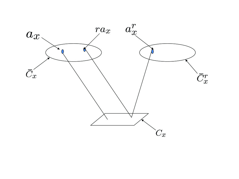
Figure 1: Relations between Elements in the base set $C_{x}$ and their Numerical Values in the Structures $\bar{C}_{x}$ and $\bar{C}^{r}_{x}.$ Here $a^{r}_{x}$ is the same number value in $\bar{C}^{r}_{x}$ as $a_{x}$ is in $\bar{C}_{x}.$ As shown by the lines they are values for different elements of $C_{x}.$ The lines also show that the $C_{x}$ element that has the value $a,$ as $a^{r}_{x}$ in $\bar{C}^{r}_{x}$, has the value $ra_{x}$ in $\bar{C}_{x}.$ Superscripts and subscripts denote structure memberships of the values.

These considerations show that the introduction of scaling between different complex number structures distinguishes a new relation, ”correspondence” from that of ”same as”. The number value $ra_{x}$ in $\bar{C}_{x}$ that corresponds to the number value $a{r}_{x}$ in $\bar{C}^{r}_{x}$ is different from the number value $a_{x}$ in $\bar{C}_{x}$ that is the same value as is $a^{r}_{x}$ in $\bar{C}^{r}_{x}.$

The setup described here collapses to the usual setup with one complex number structure at all points if $r_{y,x}=1$ everywhere. This corresponds to the usual case in which the concepts of ”correspondence” and ”same as” coincide. Also $\bar{C}^{r}_{x}=\bar{C}_{x}$ and $W^{y}_{r}=W^{r}_{x}=F_{x,y}=1.$ It follows that $\bar{C}_{x}$ for any $x$ is the same as $\bar{C}_{y}$ for any $y\neq x.$ This is equivalent to saying that $\bar{C}_{x}$ is independent of $x.$

The numbers $r_{y,x}$ and $r_{x,y}$ are associated with opposite directions of the link between sites $x$ and $y,$ with $r_{y,x}$ for the direction from $x$ to $y$ and $r_{x,y}$ for the direction from $y$ to $x.$ One would like to compare the two numbers. However, they cannot be directly compared because $r_{y,x}$ is a number in $\bar{C}_{x}$ and $r_{x,y}$ is a number in $\bar{C}_{y}.$

A comparison can be made between $r_{y,x}$ and $(r_{x,y})_{x}=F^{-1}_{y,x}r_{x,y},$ which is the same number in $\bar{C}_{x}$ as $r_{x,y}$ is in $\bar{C}_{y}.$ Since $(r_{x,y})_{x}$ and $r_{y,x}$ belong to opposite directions of the same link, it is reasonable to assume that $(r_{x,y})_{x}r_{y,x}=1_{x}$ or

$$(r_{x,y})_{x}=r_{y,x}^{-1_{x}}.$$ (13)

The equivalent relation for $\bar{C}_{y}$ is $(r_{y,x})_{y}=r_{x,y}^{-1_{y}}.$

So far the description of relations between complex number fields has been limited to elements of the fields. However, it can be extended to terms and more complicated functions. For example, consider the term $(a^{r}_{x})^{m}/(b^{r}_{x})^{n}$ in $\bar{C}^{r}_{x}.$ The representation of this term in $\bar{C}_{x}$ is given by replacing the factors and the operations in $\bar{C}^{r}_{x}$ by their equivalents in $\bar{C}_{x}$ as given in Eq. 11.

The term $(a^{r}_{x})^{m}$ has $m$ factors and $m-1$ multiplications. These combine to give a factor $r$ so that the value $(a^{r}_{x})^{m}$ in $\bar{C}^{r}_{x}$ is the value $ra_{x}^{m}$ in $\bar{C}_{x}.$ Combining this with the expression $(b^{r}_{x})^{n}=rb_{x}^{n}$ for the denominator, and a factor of $r$ arising from the solidus that represents division, gives the result

$$\frac{(a^{r}_{x})^{m}}{(b^{r}_{x})^{n}}\mbox{}^{r}_{x}=r\frac{a_{x}^{m}}{b_{x}^{n}}\mbox{}_{x}.$$ (14)

Since this applies to each term in a power series, it applies to the series as a whole. As a result, any analytic function $f^{r}_{x}$ on $\bar{C}^{r}_{x}$ corresponds to the function, $f_{x},$ in $\bar{C}_{x}$ multiplied by $r.$ That is

$$f^{r}_{x}(z^{r}_{x})=rf_{x}(z_{x}).$$ (15)

An example of this is given by the exponential $e^{z}$ as a function of the argument, $z.$ The representation of the $\bar{C}^{r}_{x}$ exponential, $e^{a^{r}_{x}},$ in $\bar{C}_{x}$ is given by $re^{a_{x}}.$ This can be understood from a power series expansion as

$$e^{a^{r}_{x}}=\sum_{n}\frac{(a^{r}_{x})^{n}}{n^{r}_{x}!}=r\sum_{n}\begin{array}[]{c}a_{x}^{n}\\ \overline{n_{x}!}\end{array}.$$

This says that the element of $C$ that has value $e^{a}$ in $\bar{C}^{r}_{x}$ has value $re^{a}$ in $\bar{C}_{x}.$

This can be extended to the $\bar{C}_{x}$ representation of equations in $\bar{C}^{r}_{x}.$ The above shows that $f^{r}_{x}(a^{r}_{x})=b^{r}_{x}$ is the same equation in $\bar{C}^{r}_{x}$ as $f_{x}(a_{x})=b_{x}$ is in $\bar{C}_{x}.$ This follows from

$$f^{r}_{x}(a^{r}_{x})=b^{r}_{x}\Leftrightarrow rf_{x}(a_{x})=rb_{x}\Leftrightarrow f_{x}(a_{x})=b_{x}.$$ (16)

This result is important because it shows that the local representations, in $\bar{C}_{x},$ of equations in $\bar{C}_{y}$ are the same equations as those in $\bar{C}_{x}$ that are obtained by parallel transformation of equations in $\bar{C}_{y}.$

As was noted before, the relations between the basic operations in $\bar{C}^{r}_{x}$ and those in $\bar{C}_{x},$ as seen in Eq. 11, must be such that $\bar{C}_{x}$ satisfies the complex number axioms [19] if and only if $\bar{C}^{r}_{x}$ satisfies the axioms. The validity of this requirement is a consequence of the fact that all the complex number axioms are equations. As was seen above, equations are valid in $\bar{C}^{r}_{x}$ if and only if their corresponding representations in $\bar{C}_{x}$ are valid.

A couple of examples of proofs for individual axioms are sufficient, as proofs to the other axioms are similar. For the axiom, $a\times a^{-1}=1,$ one has the following equivalences:

$$\begin{array}[]{l}a^{r}_{x}\times^{r}_{x}(1^{r}_{x}\div^{r}_{x}a^{r}_{x})=1^{r}_{x}\Leftrightarrow(ra_{x})\times^{r}_{x}(r1_{x})\div^{r}_{x}(ra_{x})=(r1_{x})\\ \\ \Leftrightarrow(ra_{x})(\frac{\textstyle\times_{x}}{\textstyle r}\mbox{}_{x})(r1_{x})(\frac{\textstyle r}{\textstyle ra_{x}}\mbox{}_{x})=r1_{x}\Leftrightarrow a_{x}\times_{x}(1_{x}\div_{x}a_{x})=1_{x}.\end{array}$$

Here Eq.11 was used to obtain these equivalences. For algebraic closure one can show that $a_{x}$ is the solution of a polynomial equation $P_{x}(z)=0$ in $\bar{C}_{x}$ if and only if $a^{r}_{x}$ is a solution of the corresponding polynomial equation $P^{r}_{x}(z^{r}_{x})=0$ in $\bar{C}^{r}_{x}.$

The involution axiom $(a^{*})^{*}=a$ is another example. From Eq. 11 one has

$$((a^{r}_{x})^{*^{r}_{x}})^{*^{r}_{x}}=((ra_{x})^{*^{r}_{x}})^{*^{r}_{x}}=(r(a_{x}^{*_{x}}))^{*^{r}_{x}}=r(a_{x})^{*_{x}*_{x}}.$$ (17)

From this one obtains the equivalences

$$(a^{r}_{x})^{*^{r}_{x}*^{r}_{x}}=a^{r}_{x}\Leftrightarrow(r(a_{x}^{*_{x}}))^{*^{r}_{x}}=a^{r}_{x}\Leftrightarrow r(a_{x})^{*_{x}*_{x}}=ra_{x}\Leftrightarrow(a_{x}^{*_{x}})^{*_{x}}=a_{x}.$$

3 Gauge Fields

The association of different complex number structures to space time points can be represented as a field, $\mathfrak{F},$ over space time of complex number structures. The association is given by $\mathfrak{F}:x\rightarrow\bar{C}_{x}.$

From the viewpoint of an observer at $x$ for whom the elements of $\bar{C}_{x}$ are the complex numbers, there is a local representation, $\mathfrak{F}_{x},$ of the field, $\mathfrak{F}.$ This consists of the set of local representations of $\bar{C}_{y}$ on $\bar{C}_{x}$ for all space time points $y$, not just those that are neighbors of $x.$ For points distant from $x$ the superscript $r_{y,x}$ in $\bar{C}^{r_{y,x}}_{x}$ is replaced by an integral over paths from $x$ to $y.$ These are discussed in the next subsection. Here the map, $W^{r}_{x},$ is a connection, or element of the tangent space on $\mathfrak{F}_{x}.$

The $W^{r_{y,x}}_{x}$ are elements of the gauge group $GL(1,R).$ Gauge fields enter through the representation of $W^{r}_{x}$ as

$$W^{r}_{x}=e^{\vec{A}(x)\cdot\hat{\nu}dx}=e^{A_{\mu}(x)dx^{\mu}}.$$ (18)

(Sum over $\mu$ implied.) Here $y=x+\hat{\nu}dx$ is a neighbor point of $x$ and $\vec{A}(x)$ is a real valued gauge field with four space time components $A_{\mu}(x).$ These components are real numbers in $\bar{C}_{x}$ and are associated with the link from $x$ to $y.$

Since $W^{r}_{x}a_{x}=r_{y,x}a_{x},$ Eqs. 9 and 11, one has

$$W^{r}_{x}a_{x}=e^{\vec{A}(x)\cdot\hat{\nu}dx}a_{x}.$$ (19)

This gives

$$r_{y,x}=e^{\vec{A}(x)\cdot\hat{\nu}dx},$$ (20)

which is a repetition of Eq. 3.

One can use the relation between $r_{y,x}$ and $(r_{x,y})_{x}$ to obtain a corresponding relation for the gauge field for $(r_{x,y})_{x}$. From $r_{y,x}(r_{x,y})_{x}=1_{x}$ one has

$$(r_{x,y})_{x}=1_{x}/r_{y,x}=e^{-\vec{A}(x)\cdot\hat{\nu}dx}.$$ (21)

this shows that if $\vec{A}(x)$ is associated with the link from $x$ to $y$, then $-\vec{A}(x)$ is associated with the same link in the opposite direction. In either case the components of $\vec{A}(x)$ are real number values in $\bar{C}_{x}.$

To first order in small quantities, $W^{r}_{x}$, or $r_{y,x},$ ($W^{r}_{x}$ and $r_{y,x}$ are used interchangeably here) can be expressed by

$$W^{r}_{x}=r_{y,x}=1+\vec{A}(x)\cdot\hat{\nu}dx.$$ (22)

This shows that for $y$ a neighbor point of $x,$ $r_{y,x}$ corresponds to a scale change factor, $1+\vec{A}(x)\cdot\hat{\nu}dx,$ in going from $\bar{C}^{r}_{x}$ to $\bar{C}_{x}.$

3.1 Representations of Numbers at Distant Points.

So far the description is limited to $x$ representations of number structures at neighbor points $y.$ This needs to be extended to the case where $y$ is arbitrary. The fact that number values associated with different points belong to different complex number structures needs to be taken into account.

To begin, consider a two step path $x\rightarrow y\rightarrow z$ where $y=x+\hat{\nu}_{x}\Delta_{x}$ and $z=y+\hat{\nu}_{y}\Delta_{y}.$ Subscripts will be left off of the small quantity, $\Delta,$ because it is the same number at $y$ as at $x$ ($\Delta_{y}=F_{y,x}(\Delta_{x})=\Delta$). Let $a_{z}$ denote a number in $\bar{C}_{z}.$ The goal is to find the number in $\bar{C}_{x}$ that corresponds to $a_{z}.$

Here and from now on, number values will often be referred to as numbers. The reason is that as it will be clear from context whether one is referring to elements of a base set or the values the elements take in a given structure. In cases where it is not clear, number value will be used.

From Eqs. 11 and 8 one sees that the number in $\bar{C}_{y}$ that corresponds to $a_{z}$ is $(W_{r_{z,y}}^{z})^{-1}(a_{z})$. It follows that the number in $\bar{C}_{x}$ that corresponds to $a_{z}$ is

$$\begin{array}[]{l}(W_{r_{y,x}}^{y})^{-1}((W_{r_{z,y}}^{z})^{-1}(a_{z}))=(W_{r_{y,x}}^{y})^{-1}(r_{z,y}\times_{y}a_{y})\\ \\ \hskip 28.45274pt=W^{r_{y,x}}_{x}([r_{z,y}]_{x}a_{x})=r_{y,x}[r_{z,y}]_{x}a_{x}.\end{array}$$ (23)

Here $[r_{z,y}]_{x}=F_{x,y}(r_{z,y})$ is the same number in $\bar{C}_{x}$ as $r_{z,y}$ is in $\bar{C}_{y}.$

The gauge field expression for $r_{y,x}[r_{z,y}]_{x}a_{x}$ is

$$r_{y,x}[r_{z,y}]_{x}a_{x}=e^{\vec{A}(y)_{x}\cdot\hat{\nu}_{y}\Delta+\vec{A}(x)\cdot\hat{\nu}_{x}\Delta}a_{x}.$$ (24)

Here $a_{x}=F_{x,z}a_{z}$ is the same number in $\bar{C}_{x}$ as $a_{z}$ is in $\bar{C}_{z}.$ The commutativity of $\vec{A}(x)$ with $\vec{A}(y)_{x}$ is used here along with the observation that

$$[r_{z,y}]_{x}=[e^{\vec{A}(y)\cdot\hat{\nu}_{y}\Delta}]_{x}=e^{\vec{A}(y)_{x}\cdot\hat{\nu}_{y}\Delta}.$$ (25)

The components, $A_{\mu}(y)_{x},$ of $\vec{A}(y)_{x}$ are the same numbers in $\bar{C}_{x}$ as the $A_{\mu}(y)$ are in $\bar{C}_{y}.$

The notation used here is that for functions, such as $A_{\mu}(y),$ the subscript $x,$ as in $A_{\mu}(y)_{x},$ denotes the same number value in $\bar{C}_{x}$ as $A_{\mu}(y)$ is in $\bar{C}_{y}.$ For number values with subscripts, such as $r_{z,y},$ square brackets and a subscript, such as $[r_{z,y}]_{x}$ are used to denote structure membership.

Extension of the two step result to an $n$ step path $P$ where $P(0)=x_{0}=x,P(n)=x_{n}=y,P(j)=x_{j}$ and $x_{j+1}=x_{j}+\hat{\nu}_{j}\Delta$ for $0\leq j\leq n$ gives

$$W^{x}_{y}(a_{y})=r^{P}_{y,x}a_{x}$$ (26)

where

$$r^{P}_{y,x}=\prod_{j=0}^{n-1}[r_{x_{j+1},x_{j}}]_{x}.$$ (27)

Here $W^{x}_{y}(a_{y})$ denotes the representation of $a_{y}$ in $\bar{C}_{x}.$ The gauge field expression for $r^{P}_{y,x}$ is

$$r^{P}_{y,x}=\exp(\sum_{j=0}^{n-1}[\vec{A}(x_{j})\cdot\hat{\nu}_{j}\Delta_{x_{j}}]_{x}).$$ (28)

For a continuous path $P$ from $x$ to $y$ Eq. 28 becomes

$$r^{P}_{y,x}=\exp\{\int_{0}^{1}\vec{A}(P(s))_{x}\cdot[\frac{dP(s)}{ds}]_{x}ds\}.$$ (29)

The path is parameterized by a variable $s,$ $0\leq s\leq 1,$ where $P(0)=x$ and $P(1)=y.$ An ordering of the integrand variables is not needed because the $\vec{A}(y)_{x}$ commute for different $y.$

The subscript $x$ in the integrand and on $\vec{A}(P(s))_{x}$ indicate that the integral is defined in $\bar{C}_{x}$ and that the components, $A_{\mu}(P(s))_{x}$, which are numbers in $\bar{C}_{x},$ are the same numbers in $\bar{C}_{x}$ as the numbers $A_{\mu}(P(s))$ are in $\bar{C}_{P(s)}.$ This is expressed by

$$A_{\mu}(P(s))_{x}=F_{x,P(s)}A_{\mu}(P(s)).$$ (30)

The derivative components, $[dP_{\mu}(s)/ds]_{x},$ which are the same numbers in $\bar{C}_{x}$ as $dP_{\mu}(s)/ds,$ are in $\bar{C}_{P(s)}$ are related to $dP_{\mu}(s)/ds$ by

$$[\frac{dP_{\mu}(s)}{ds}]_{x}=F_{x,P(s)}\frac{dP_{\mu}(s)}{ds}.$$ (31)

$r^{P}_{y,x}$ can be expressed as the exponential of a line integral along the path $P$ as in

$$r^{P}_{y,x}=\exp(\int_{P}\vec{A}(z)_{x}\vec{dz}).$$ (32)

The subscript $x$ indicates that the integral is defined in $\bar{C}_{x}.$

3.2 Derivatives and Integrals over Space Time

The dependence of $\bar{C}_{x}$ on $x$ has an effect on derivatives and integrals of functions over space time. To see this let $\Phi(x)$ be a function over space time such that for each $x,$ $\Phi(x)$ is a number in $\bar{C}_{x}.$ As was noted in the introduction for Eq. 1, the problems of the the usual derivative,

$$\partial_{\mu,x}\Phi=\frac{\Phi(x+dx^{\mu})-\Phi(x)}{\partial{x^{\mu}}}$$ (33)

can be avoided by defining a local representation of $\bar{C}_{x+dx^{\mu}}$ on $\bar{C}_{x}$ as in Eq. 12. This enables the derivative to be expressed entirely within $\bar{C}_{x}$ as, Eq. 4,

$$D_{\mu,x}\Phi=\frac{r_{x+dx^{\mu},x}\Phi(x+dx^{\mu})_{x}-\Phi(x)}{\partial{x}^{\mu}}$$ (34)

where

$$\Phi(x+dx^{\mu})_{x}=F_{x+dx^{\mu},x}^{-1}\Phi(x+dx^{\mu})$$ (35)

is the same number value in $\bar{C}_{x}$ as $\Phi(x+dx^{\mu})$ is in $\bar{C}_{x+dx^{\mu}}.$ The term, $r_{x+dx^{\mu},x}\Phi(x+dx^{\mu})_{x},$ in Eq. 34, denotes the number in $\bar{C}_{x}$ that corresponds to the number $\Phi(x+dx^{\mu})$ in $\bar{C}_{x+dx^{\mu}}.$

Expressing $r_{x+dx^{\mu},x}$ in terms of gauge potentials and expanding to first order in $dx^{\mu}$ gives

$$D_{\mu,x}\Phi=(\partial^{\prime}_{\mu,x}+A_{\mu}(x))\Phi(x)$$ (36)

where

$$\partial^{\prime}_{\mu,x}\Phi=\frac{\Phi(x+dx^{\mu})_{x}-\Phi(x)}{\partial{x}^{\mu}}$$ (37)

is a repetition of Eq. 2.

The presence of the gauge field, $\vec{A}(x),$ is a consequence of the freedom to choose complex number structures, one for each $x.$ If $\vec{A}(x)=0$ everywhere, then the complex number structures would all be the same and they can be collapsed into one structure. In this case $F_{y,x}=1$ and

$$D_{\mu,x}\Phi=\partial^{\prime}_{\mu,x}\Phi=\partial_{\mu,x}\Phi.$$ (38)

Similar considerations hold for space time integrals. The usual expression $\int\Phi(x)d^{4}x.$ is not defined because it corresponds to adding together values of $\Phi(x)$ in different $\bar{C}_{x}.$ One way to handle this is to choose a point $x$ and the associated $\bar{C}_{x}$ and map all the values of $\Phi(y)$ to their representations in $\bar{C}_{x}.$ The integral is then defined on $\bar{C}_{x}.$ This is done by replacing $\Phi(y)$ by its local representative in $\bar{C}_{x},$ which is

$$W^{x}_{y}(\Phi(y))=r^{P}_{y,x}F^{-1}_{y,x}(\Phi(y))=r^{P}_{y,x}\Phi(y)_{x}.$$ (39)

Here $\Phi(y)_{x}$ is the $F$ same number in $\bar{C}_{x}$ as $\Phi(y)$ is in $\bar{C}_{y}$ and $P$ is a path from $x$ to $y.$ $c^{P}_{y,x}$ is given by Eq. 32.

Putting this together gives

$$\int_{x}\Phi=\int r^{P}_{y,x}\Phi(y)_{x}d^{4}y=\int\exp(\int_{P}\vec{A}(z)_{x}\vec{dz})\Phi(y)_{x}d^{4}y.$$ (40)

This expression has the disadvantage that it depends on paths from all space time points to $x$. One might be able to handle this by carrying out some type of Feynman path integral. This can be avoided if one assumes that the $r^{P}_{y,x}$ are integrable, or path independent. In this case Eq. 40 becomes

$$\int_{x}\Phi=\int r_{y,x}\Phi(y)_{x}d^{4}y=\int(e^{\int^{y}_{x}\vec{A}})\Phi(y)_{x}d^{4}y.$$ (41)

Here the line integral of $\vec{A}$ is independent of the path choice. However, it remains to be seen if the assumption of integrability is valid or not.

There remains the dependence on $x$ indicated by the subscript $x$ on $\int_{x}\Phi.$ It is suspected that the results are independent of $x.$ This is based on the observation that all the results obtained so far depend on the relation between systems at $x$ and $y$ and not on the location of $x.$ However, this remains to be investigated.

4 Hilbert Spaces

So far, complex number structures have been considered by themselves. However, there are many types of mathematical systems that are based on the real or complex numbers as underlying scalar fields. Vector spaces based on complex numbers are examples of this type of mathematical system. For these spaces, it would be expected that the differences between complex number systems at different space time points would have an effect on vectors and vector spaces assigned to different points.

Here this is seen to be the case for Hilbert spaces as examples of vector spaces. Let $\bar{H}_{x},\bar{C}_{x}$ be an $n$ dimensional Hilbert space and a complex number field at point $x.$ As a structure

$$\bar{H}_{x}=\{H_{x},+_{x},-_{x},\cdot_{x},\langle-,-\rangle_{x},\psi_{x}\}$$ (42)

where $H_{x}$ is a base set, $+_{x}$ and $-_{x}$ denote linear addition and subtraction, $\cdot_{x}$ denotes multiplication of a vector by a scalar in $\bar{C}_{x},$ and $(-,-)_{x}$ denotes the scalar product with values in $\bar{C}_{x}.$ $\psi_{x}$ denotes an arbitrary vector in $\bar{H}_{x}.$

The basic operations shown in Eq. 42 must satisfy the axioms for a Hilbert space. These describe a complex inner product vector space that is complete in the norm [10].

The freedom of basis choices for Hilbert spaces at different space time points [1] can be expressed here by representing the parallel transform, $U_{y,x},$ from $\bar{H}_{x}$ to $\bar{H}_{y}$ as a product of two factors, as in

$$\bar{H}_{y}=U_{y,x}\bar{H}_{x}=\mathfrak{V}_{y,x}V_{y,x}\bar{H}_{x}.$$ (43)

The reason that the unitary operator, $U_{y,x},$ is a product of two factors is that $U_{y,x}$ cannot be represented as a unitary matrix of complex number entries. If $U_{y,x}=\{a_{i,j,x}\}$ where the $a_{i,j,x}$ are numbers in $\bar{C}_{x},$ then for any vector $\psi_{x}$ in $\bar{H}_{x},$ $U_{y,x}\psi_{x}=\sum_{i,j}|i\rangle_{x}a_{i,j,x}\langle j,\psi_{x}\rangle_{x}$ is a vector in $\bar{H}_{x}.$ It is not a vector in $\bar{H}_{y}.$ This is the case even if $\bar{C}_{x}$ is replaced by $\bar{C},$ which is common to both $\bar{H}_{x}$ and $\bar{H}_{y}.$

The unitary operator $V_{y,x}$ maps a set of basis vectors to a transformed basis in $\bar{H}_{x}$ that is the $\bar{H}_{x}$ representation of a basis in $\bar{H}_{y}.$ If $|j\rangle_{x}$ is a basis vector in $\bar{H}_{x}$ then $V_{y,x}|j\rangle_{x}$ is the transformed vector that is the representation of $|j\rangle_{y}$ in $\bar{H}_{x}.$ $\mathfrak{V}_{y,x}$ maps the transformed basis to the corresponding basis in $\bar{H}_{y}$ that is the same as the original basis in $\bar{H}_{x}.$ That is, $|j\rangle_{y}=U_{y,x}|j\rangle_{x}.$

Eq. 43 describes parallel transformations from $\bar{H}_{x}$ to $\bar{H}_{y}$. However it does not include the corresponding changes in going from $\bar{C}_{x}$ to $\bar{C}_{y}.$ These are taken into account by considering the overall transformation $\bar{H}_{x},\bar{C}_{x}$ to $\bar{H}_{y},\bar{C}_{y}$ as a three step process. The first step takes $\bar{H}_{x}$ to $V_{y,x}\bar{H}_{x}.$ $\bar{C}_{x}$ remains unchanged.

The second step takes $V_{y,x}\bar{H}_{x}$ to $\mathfrak{V}^{r}_{x}V_{y,x}\bar{H}_{x}=\bar{H}^{r}_{x}$ and $\bar{C}_{x}$ to $W^{r}_{x}\bar{C}_{x}=\bar{C}^{r}_{x}$ and the third step takes $\bar{H}^{r}_{x}$ and $\bar{C}^{r}_{x}$ to $\bar{H}_{y}=\mathfrak{V}_{y,x}\bar{H}^{r}_{x}$ and $\bar{C}_{y}=W^{y}_{r}\bar{C}^{r}_{x}.$ Here $\bar{H}^{r}_{x}$ and $\bar{C}^{r}_{x}$ are the respective local representations of $\bar{H}_{y}$ and $\bar{C}_{y}$ on $\bar{H}_{x}$ and $\bar{C}_{x}.$ A summary of the three steps is given by

$$\begin{array}[]{c}\bar{H}_{x}\\ \bar{C}_{x}\end{array}\rightarrow\begin{array}[]{c}V_{y,x}\bar{H}_{x}\\ \bar{C}_{x}\end{array}\rightarrow\begin{array}[]{c}\mathfrak{V}^{r}_{x}V_{y,x}\bar{H}_{x}\\ W^{r}_{x}\bar{C}_{x}\end{array}=\begin{array}[]{c}\bar{H}^{r}_{x}\\ \bar{C}^{r}_{x}\end{array}\rightarrow\begin{array}[]{c}\mathfrak{V}^{y}_{r}\bar{H}^{r}_{x}\\ W^{y}_{r}\bar{C}^{r}_{x}\end{array}=\begin{array}[]{c}\mathfrak{V}_{y,x}V_{y,x}\bar{H}_{x}\\ F_{y,x}\bar{C}_{x}\end{array}=\begin{array}[]{c}\bar{H}_{y}\\ \bar{C}_{y}\end{array}.$$ (44)

Here $W^{r}_{x}$ and $W^{y}_{r}$ are given by Eqs. 7-9.

$\bar{H}^{r}_{x}$ has the structure representation

$$\bar{H}^{r}_{x}=\{H_{x},\pm^{r}_{x},\cdot^{r}_{x},\langle-,-\rangle^{r}_{x},\psi^{r}_{x}\}.$$ (45)

$H_{x}$ is the same base set as that in $\bar{H}_{x},$ $\pm^{r}_{x}$ denotes addition and subtraction of vectors, $\cdot^{r}_{x}$ and $\langle-,-\rangle^{r}_{x}$ denote scalar vector multiplication and scalar product, and $\psi^{r}_{x}$ denotes an arbitrary vector in $\bar{H}^{r}_{x}.$ Also $\bar{C}^{r}_{x}$ is given by Eq. 6, and, as before, $r=r_{y,x}$.

The map $\mathfrak{V}^{r}_{x}$ is defined by

$$\begin{array}[]{c}\mathfrak{V}^{r}_{x}V_{y,x}\psi_{x}=\psi^{r}_{x}\\ \\ \mathfrak{V}^{r}_{x}(V_{y,x}\psi_{x}\pm_{x}V_{y,x}\phi_{x})=(\mathfrak{V}^{r}_{x}V_{y,x}\psi_{x})\pm^{r}_{x}(\mathfrak{V}^{r}_{x}V_{y,x}\phi_{x})=\psi^{r}_{x}\pm^{r}_{x}\phi^{r}_{x}\\ \\ \mathfrak{V}^{r}_{x}(\alpha_{x}\cdot_{x}V_{y,x}\psi_{x})=(W^{r}_{x}\alpha_{x})\cdot^{r}_{x}\mathfrak{V}^{r}_{x}V_{y,x}\psi_{x}=\alpha^{r}_{x}\cdot^{r}_{x}\psi^{r}_{x}\\ \\ \mathfrak{V}^{r}_{x}\langle V_{y,x}\psi_{x},V_{y,x}\phi_{x}\rangle_{x}=\langle\mathfrak{V}^{r}_{x}V_{y,x}\psi_{x},\mathfrak{V}^{r}_{x}V_{y,x}\phi_{x}\rangle_{x}^{r}=\langle\psi^{r}_{x},\phi^{r}_{x}\rangle^{r}_{x}.\end{array}$$ (46)

As was the case of the complex number structures, the representation of $\bar{H}_{y},\bar{C}_{y}$ on $\bar{H}_{x},\bar{C}_{x}$ is obtained by giving the definitions of the vectors and basic operations in $\bar{H}^{r}_{x}$ in terms of the vectors and basic operations in $\bar{H}_{x}.$ The resulting representation of $\bar{H}^{r}_{x}$ must also be such that $\bar{H}^{r}_{x}$ satisfies the Hilbert space axioms if and only if $\bar{H}_{x}$ satisfies the axioms.

The definitions are made specific by first giving a specific representation of the vector $\psi^{r}_{x}$ in $\bar{H}_{x}.$ The development so far suggests that both $V_{y,x}$ and the dependence of the complex numbers on $x$ should be included. This can be achieved by the specific correspondence

$$(\psi^{r}_{x})_{x}=\mathfrak{V}^{r}_{x}V_{y,x}\psi_{x}=r_{y,x}V_{y,x}\psi_{x}=e^{\vec{A}(x)\cdot\hat{\nu}dx}V_{y,x}\psi_{x}.$$ (47)

The parentheses around $\psi^{r}_{x}$ and the subscript $x$ indicate that $(\psi^{r}_{x})_{x}$ is the vector in $\bar{H}_{x}$ that corresponds to $\psi^{r}_{x}$ in $\bar{H}^{r}_{x}.$ Alternatively one can say that $(\psi^{r}_{x})_{x}$ is the local representation of $\psi_{y}$ on $\bar{H}_{x}$ where $\psi_{y}$ is the same state in $\bar{H}_{y}$ as $\psi_{x}$ is in $\bar{H}_{x}.$

Reference to Fig. 1, which also applies to other mathematical systems, such as Hilbert spaces, is useful here. It shows that the element of the base set $H_{x},$ that is the vector $\psi^{r}_{x}$ in $\bar{H}^{r}_{x},$ is the vector $r_{y,x}V_{y,x}\psi_{x}$ in $\bar{H}_{x}.$ Also the element of $H_{x}$ that is the vector $\psi^{r}_{x}$ in $\bar{H}^{r}_{x}$ is different from the element that is the same vector $\psi_{x}$ in $\bar{H}_{x}.$

The requirement that $rV_{y,x}\psi_{x}$ in $\bar{H}_{x}$, corresponds to the vector $\psi^{r}_{x}$ in $\bar{H}^{r}_{x},$ results in compensatory changes in basic operations in $\bar{H}^{r}_{x},$ expressed in terms of operations in $\bar{H}_{x}.$ The changes must be such that the structure, $\bar{H}^{r}_{x},$ satisfies the Hilbert space axioms if and only if $\bar{H}_{x}$ does.

Eq. 47 can be used to determine the relations between the Hilbert space operations in $\bar{H}_{x}$ and those in $\bar{H}^{r}_{x}.$ The representation, in $\bar{H}_{x}$ of the linear superposition operation in $\bar{H}^{r}_{x},$ is given by

$$(\pm^{r}_{x})_{x}=\pm_{x}.$$ (48)

This follows from the equivalences

$$\begin{array}[]{l}\psi^{r}_{x}\pm^{r}_{x}\phi^{r}_{x}=\theta^{r}_{x}\Leftrightarrow r_{y,x}V_{y,x}\psi_{x}(\pm^{r}_{x})_{x}r_{y,x}V_{y,x}\phi_{x}=r_{y,x}V_{y,x}\theta_{x}\\ \hskip 28.45274pt\Leftrightarrow\psi_{x}\pm_{x}\phi_{x}=\theta_{x}.\end{array}$$

For scalar vector multiplication one can use the equation, $\psi_{x}=1_{x}\cdot_{x}\psi_{x}$ in $\bar{H}_{x}$ to determine the relations. The equivalences

$$\begin{array}[]{l}\psi^{r}_{x}=1^{r}_{x}\cdot^{r}_{x}\psi^{r}_{x}\Leftrightarrow rV_{y,x}\psi_{x}=(r1_{x})(\cdot^{r}_{x})_{x}(rV_{y,x}\psi_{x})\\ \hskip 28.45274pt\Leftrightarrow\psi_{x}=1_{x}\cdot_{x}\psi_{x}\end{array}$$

require that $r(\cdot^{r}_{x})_{x}=\cdot_{x},$ or

$$(\cdot^{r}_{x})_{x}=\frac{\cdot_{x}}{r}.$$ (49)

For scalar products one requires $\langle\psi_{x}^{r},\phi_{x}^{r}\rangle^{r}_{x}$ to be the same number in $\bar{C}^{r}_{x}$ as $\langle\psi_{x},\phi_{x}\rangle_{x}$ is in $\bar{C}_{x}.$ This is based on the fact that $\psi_{x}^{r}$ is the same vector in $\bar{H}^{r}_{x}$ as $\psi_{x}$ is in $\bar{H}_{x}.$

This requirement (footnote on page 5) is expressed by the equation equivalences,

$$\begin{array}[]{l}\langle\psi_{x}^{r},\phi_{x}^{r}\rangle^{r}_{x}=d^{r}_{x}\Leftrightarrow(\langle\psi_{x}^{r},\phi_{x}^{r}\rangle^{r}_{x})_{x}=rd_{x}\\ \hskip 28.45274pt\Leftrightarrow\langle\psi_{x},\phi_{x}\rangle_{x}=d_{x}.\end{array}$$ (50)

Here $(\langle\psi_{x}^{r},\phi_{x}^{r}\rangle^{r}_{x})_{x}$ is the representation, in $\bar{C}_{x},$ of the number value, $\langle\psi_{x}^{r},\phi_{x}^{r}\rangle^{r}_{x},$ in $\bar{C}^{r}_{x}.$

It remains to determine the relationship between $(\langle\psi_{x}^{r},\phi_{x}^{r}\rangle^{r}_{x})_{x}$ and $\langle(\psi_{x}^{r})_{x},(\phi_{x}^{r})_{x}\rangle_{x}.$ From Eq. 47 one has

$$\langle(\psi_{x}^{r})_{x},(\phi_{x}^{r})_{x}\rangle_{x}=\langle rV_{y,x}\psi_{x},rV_{y,x}\phi_{x}\rangle_{x}=r^{2}\langle\psi_{x},\phi_{x}\rangle_{x}.$$ (51)

Use of Eq. 50 gives

$$\langle(\psi_{x}^{r})_{x},(\phi_{x}^{r})_{x}\rangle_{x}=r(\langle\psi_{x}^{r},\phi_{x}^{r}\rangle^{r}_{x})_{x}.$$ (52)

These relations do not conflict with the usual properties of scalar products. For example, the $\bar{C}^{r}_{x}$ norm of a vector is the same number as is the corresponding norm in $\bar{C}_{x}.$ This can be seen from Eq. 50 which gives

$$\langle\psi^{r}_{x},\psi^{r}_{x}\rangle^{r}_{x}=1^{r}_{x}\Leftrightarrow\langle\psi_{x},\psi_{x}\rangle_{x}=1_{x}.$$

Norm preservation occurs because $1^{r}_{x}=r1_{x}$ is the multiplicative identity in $\bar{C}^{r}_{x}.$

It follows from these relations that the representation of $\bar{H}_{y}$ on $\bar{H}_{x}$ can be described as the structure,

$$\begin{array}[]{l}\bar{H}^{r}_{x}=\{H_{x},\pm^{r}_{x},\cdot^{r}_{x},\langle-,-\rangle^{r}_{x},\psi^{r}_{x}\}\\ \hskip 28.45274pt=\{H_{x},\pm_{x},\frac{\textstyle\cdot_{x}}{\textstyle r},\frac{\textstyle\langle-,-\rangle_{x}}{\textstyle r},rV_{y,x}\psi_{x}\}.\end{array}$$ (53)

The first line in the equation is a repetition of Eq. 45. The second line in Eq. 53 gives a representation of the elements of the structure $\bar{H}^{r}_{x}$ in terms of elements of $\bar{H}_{x}.$ It is also part of a local representation of $\bar{H}_{y},\bar{C}_{y}$ on $\bar{H}_{x},\bar{C}_{x}.$ Thus $rV_{y,x}\psi_{x},\langle-,-\rangle_{x}/r,\cdot_{x}/r$ are representations of $\psi^{r}_{x},\langle-,-\rangle^{r}_{x},$ $\cdot^{r}_{x}$ in $\bar{H}_{x}$ and local representations of $\psi_{y},\langle-,-\rangle_{y},\cdot_{y}$ in $\bar{H}_{x}.$

The blanks in $\langle-,-\rangle^{r}_{x}$ denote vectors $\psi^{r}_{x},\phi^{r}_{x}$, and the blanks in $\langle-,-\rangle_{x}$ denote vectors $rV_{y,x}\psi_{x},rV_{y,x}\phi_{x}.$ Eq. 52 was used to obtain the relation between the scalar products in the two representations of $\bar{H}^{r}_{x}.$

5 Gauge Theories

The material presented so far forms a base for further explorations into the possible effect of the gauge field, $\vec{A}(x),$ in physics and mathematics. One direction to explore is the description of gauge theories, which have been so important in physics [1, 5, 22]. Here the discussion is limited to very elementary aspects of these theories with their associated Lagrangians. Because of the presence of different scalar structures at each space time point, the discussion is a bit more detailed than would otherwise be needed.

Let $\psi$ be a field such that, for each point $x,$ $\psi(x)$ is a vector in an $n$ dimensional Hilbert space, $\bar{H}_{x}.$ Relative to basis choices in each $\bar{H}_{x},$ $\psi$ is an $n$ component complex scalar field. Since $n$ dimensional Hilbert spaces can be represented by $n$ tuples, $\bar{C}^{n},$ of complex number fields [21], $\psi(x)$ can be thought of as an element of $\bar{C}^{n}_{x}.$

The dynamics of the fields are described by Lagrangians that include terms containing space and time derivatives of the fields. Examples include the Klein Gordon and Dirac Lagrangians as

$$\mathcal{L}(x)=\psi^{{\dagger}}(x)\partial^{\mu}_{x}\partial_{\mu,x}\psi-m^{2}\bar{\psi}(x)\psi(x)$$ (54)

and

$$\mathcal{L}(x)=\bar{\psi}(x)i\gamma^{\mu}\partial_{\mu,x}\psi-m\bar{\psi}(x)\psi(x).$$ (55)

In these expressions the derivative $\partial_{\mu,x}$ is given by Eq. 1, which is repeated here,

$$\partial_{\mu,x}\psi=\frac{\psi(x+dx^{\mu})-\psi(x)}{\partial x^{\mu}}.$$ (56)

As noted for Eq. 1, the derivative in Eq. 56 is not defined. The reasons are that subtraction is not defined between elements of $\bar{H}_{x}$ and $\bar{H}_{x+dx^{\mu}}$ and the ”no information at a distance principle” prevents an observer at $x$ from direct access to vectors at $x+dx^{\mu}.$

This problem is solved by replacing $\psi(x+dx^{\mu})$ with the vector in $\bar{H}_{x}$ that corresponds to the vector $\psi(x+dx^{\mu})^{r}_{x}$ in $\bar{H}^{r}_{x}.$ Recall that $\bar{H}^{r}_{x}$ is the local representation of $\bar{H}_{x+dx^{\mu}}$ on $\bar{H}_{x}.$

The replacement vector is given by

$$\begin{array}[]{l}(\mathfrak{V}^{\mu}_{r})^{-1}\psi(x+dx^{\mu})=\mathfrak{V}^{r}_{x}V_{\mu,x}\psi(x+dx^{\mu})_{x}\\ \\ \hskip 28.45274pt=e^{A_{\mu}(x)dx^{\mu}}V_{\mu,x}\psi(x+dx^{\mu})_{x}.\end{array}$$ (57)

Here $\psi(x+dx^{\mu})_{x}=(U_{\mu,x})^{-1}\psi(x+dx^{\mu})$ where the parallel transform operator, $U_{\mu,x},$ from $\bar{H}_{x}$ to $\bar{H}_{x+dx^{\mu}}$ is given by Eqs. 43 and 44. To save on notation, $x+dx^{\mu}$ is often replaced by $\mu$ as in $\mathfrak{V}^{\mu}_{x}.$ Also $r=r_{\mu,x}$ is the $\mu$ component of $r_{y,x}.$

The replacement vector can also be described as the vector value, in $\bar{H}_{x},$ of the element of the base set, $H_{x},$ that has the value $\psi(x+dx^{\mu})^{r}_{x}$ in $\bar{H}^{r}_{x}.$ This is to be distinguished from another base set element that has the value $\psi(x+dx^{\mu})_{x}$ in $\bar{H}_{x}.$ This is the same vector value in $\bar{H}_{x}$ as $\psi(x+dx^{\mu})^{r}_{x}$ is in $\bar{H}^{r}_{x},$ and as $\psi(x+dx^{\mu})$ is in $\bar{H}_{x+dx^{\mu}}.$

Eq. 57 is used to express the covariant derivative, $D_{\mu,x},$ as

$$D_{\mu,x}\psi=\frac{\mathfrak{V}^{r}_{x}V_{\mu,x}\psi(x+dx^{\mu})_{x}-\psi(x)}{\partial x^{\mu}}$$ (58)

as a replacement for $\partial_{\mu,x}$ in the Lagrangians. Here $\mathfrak{V}^{r}_{x}$ and $V_{\mu,x}$ account, respectively, for the freedom of choice of complex number structures and of bases in the Hilbert spaces.

In the following, the consequences of the replacement of ordinary derivatives by $D_{\mu,x}$ in Lagrangians will be described for Abelian and nonabelian gauge theory [7, 22, 23]. The gauge group for Abelian theories is $GL(1,r)\times U(1),$ and $GL(1,R)\times U(n)$ with $n>1$ for nonabelian theories. For Abelian theories, group elements $\mathfrak{V}^{r}_{x}V_{y,x}$ have Lie algebra representations as

$$\mathfrak{V}^{r_{y,x}}_{x}V_{y,x}=e^{\vec{A}(x)\cdot\hat{\nu}dx}e^{i\vec{\Gamma}(x)\cdot\hat{\nu}dx}.$$ (59)

For nonabelian theories there is an additional factor for the Lie algebra representations of elements of $SU(n).$

5.1 Abelian Gauge Theory

For Abelian theories the covariant derivative can be expressed by

$$D_{\mu,x}\psi=\frac{e^{A_{\mu}(x)dx^{\mu}}e^{i\Gamma_{\mu}(x)dx^{\mu}}\psi(x+dx^{\mu})_{x}-\psi(x)}{\partial x^{\mu}}.$$ (60)

Expansion of the exponential in $D_{\mu,x}$ to first order in small quantities gives the relation between $\partial^{\prime}_{\mu,x},$ defined in Eq. 37, and $D_{\mu,x}.$ This is

$$D_{\mu,x}\psi=(\partial^{\prime}_{\mu,x}+g_{R}A_{\mu}(x)+ig_{I}\Gamma_{\mu}(x))\psi(x).$$ (61)

Coupling constants for $\vec{A}(x)$ and $\vec{\Gamma}(x)$ have been included.

A well known requirement on a Lagrangian is that each term must be invariant under both global and local gauge transformations. Global transformations have the form $\Lambda_{x}=e^{i\phi_{x}}$ where $\phi_{x}$ is the same number in $\bar{C}_{x}$ as $\phi_{y}$ is in $\bar{C}_{y}.$

Local gauge transformations, $\Lambda(x)=e^{i\phi(x)},$ satisfy

$$F_{y,x}\Lambda(x)=(\Lambda(x))_{y}=(e^{i\phi(x)})_{y}=e^{i\phi(x)_{y}}\neq\Lambda(y)=e^{i\phi(y)}.$$ (62)

Here $\Lambda(x)$ is different for different $x$ as $\phi(x)_{y}\neq\phi(y).$

Terms in the Lagrangian containing the covariant derivative are invariant under global gauge transformations if $D_{\mu,x}\Lambda\psi=\Lambda_{x}D_{\mu,x}\psi.$ This follows from the observation that $\partial^{\prime}_{\mu,x}\Lambda_{x}=0.$ Terms are invariant under local transformations if

$$D^{\prime}_{\mu,x}\Lambda\psi=\Lambda(x)D_{\mu,x}\psi.$$ (63)

Here $D^{\prime}_{\mu,x}\Lambda\psi$ is obtained from Eq. 61 as

$$D^{\prime}_{\mu,x}\Lambda\psi=\partial^{\prime}_{\mu,x}\Lambda\psi+(g_{R}A^{\prime}_{\mu}(x)+ig_{I}\Gamma^{\prime}_{\mu}(x))\Lambda(x)\psi(x).$$ (64)

This equation and Eq. 63 are used in the standard procedure for Abelian gauge theories [22] to give

$$\begin{array}[]{l}(g_{R}A^{\prime}_{\mu}(x)+ig_{I}\Gamma^{\prime}_{\mu}(x))\Lambda(x)\psi(x)\\ \\ \hskip 28.45274pt=\Lambda(x)(g_{R}A_{\mu}(x)+ig_{I}\Gamma_{\mu}(x))\psi(x)-\partial^{\prime}_{\mu,x}(\Lambda)\psi(x).\end{array}$$ (65)

Use of $\partial^{\prime}_{\mu,x}(\Lambda)=i\partial^{\prime}_{\mu,x}(\phi(x))\Lambda(x)$ and separation of Eq. 65 into two separate equations for the real and imaginary parts gives the result that

$$A^{\prime}_{\mu}(x)=A_{\mu}(x)$$ (66)

and

$$\Gamma^{\prime}_{\mu}(x)=\Gamma_{\mu}(x)+\frac{i\Lambda^{-1}(x)\partial^{\prime}_{\mu,x}\Lambda}{g_{I}}=\Gamma_{\mu}(x)-\frac{1}{g_{I}}\partial^{\prime}_{\mu,x}\phi(x).$$ (67)

This result shows that the effect of local gauge transformations is limited to the gauge field $\Gamma_{\mu}(x)$ as $A_{\mu}(x)$ is unaffected. That is, $A_{\mu}(x)$ is gauge invariant. It follows that $\vec{A}(x)$ and $\vec{\Gamma}(x),$ correspond respectively to two gauge bosons, one for which having mass is possible, and the other which must be massless.

The dynamics of the massless boson can be added to the Lagrangian in the standard way by addition of a gauge invariant Yang Mills term,

$$-\frac{1}{4}G_{I,\mu,\nu}G^{\mu,\nu}_{I}$$ (68)

for $\Gamma_{\mu}(x).$ Here

$$G_{I,\mu,\nu}=\partial^{\prime}_{\mu,x}\Gamma_{\nu}(x)-\partial^{\prime}_{\nu,x}\Gamma_{\mu}(x).$$ (69)

Addition of the term of Eq. 68 and a mass term for the field, $A_{R,\mu}(x),$ in the Dirac Lagrangian gives

$$\begin{array}[]{l}\mathcal{L}(x)=\bar{\psi}i\gamma^{\mu}(\partial^{\prime}_{\mu,x}+g_{R}A_{\mu}(x)+ig_{I}\Gamma_{\mu}(x))\psi-m\bar{\psi}\psi\\ \\ \hskip 28.45274pt-\frac{1}{2}\lambda^{2}A^{\mu}(x)A_{\mu}(x)-\frac{1}{4}G_{I,\mu,\nu}G^{\mu,\nu}_{I}.\end{array}$$ (70)

Except for the terms involving $A_{\mu}(x),$ this has the same form as the Lagrangian for QED. This shows that, for this setup, the QED Lagrangian, is obtained by setting $\vec{A}(x)=0$ for all $x.$

5.2 Nonabelian Gauge Theory

Here the simplest case for a nonabelian gauge theory is considered. Let $\psi$ be a two dimensional field where for each $x,$ $\psi(x)$ is a vector in a two dimensional Hilbert space $\bar{H}_{x}.$ Relative to bases in the spaces $\bar{H}_{x},$ $\psi$ is a two dimensional complex scalar field.

The Dirac and Klein Gordon Lagrangians have the form as shown in Eqs. 54 and 55 with $D_{\mu,x}$ replacing $\partial_{\mu,x}.$ For each $x$ the scalar product

$$\bar{\psi}(x)\cdot\psi(x)=\bar{\psi}(x)^{1}\psi(x)^{1}+\bar{\psi}(x)^{2}\psi(x)^{2}$$ (71)

is a number in $\bar{C}_{x}.$ As was the case for Abelian gauge theory $D_{\mu,x}$ is given by Eq. 58. However, $V_{\mu,x},$ as an element of $U(2),$ is given by

$$V_{\mu,x}=e^{i\Gamma_{\mu}(x)dx^{\mu}}e^{-i\vec{\Omega}_{\mu}(x)\cdot\frac{\tilde{\tau}}{2}dx^{\mu}}.$$ (72)

Here

$$\vec{\Omega}_{\mu}(x)\cdot\tilde{\tau}=\Omega_{\mu}^{j}(x)\tau_{j}$$ (73)

where the $j$ indices are summed over. $\vec{\Omega}_{\mu}$ is a three component vector gauge field whose components, $\Omega_{\mu}^{j},$ represent the three vector gauge bosons, and the $\tau_{j}$ are the generators of the Lie algebra $su(2).$ As Pauli spin operators, the $\tau_{j}$ satisfy the commutation rule,

$$[\frac{\tau_{j}}{2},\frac{\tau_{k}}{2}]=i\xi_{jkl}\frac{\tau_{l}}{2}\hskip 56.9055ptj,k,l=1,2,3.$$ (74)

The structure constant, $\xi_{jkl},$ is antisymmetric under exchange of indices. At each point $x$ the vector components, $\Omega_{\mu}^{j}(x),$ are real numbers in $\bar{C}_{x}$ and the elements of the Pauli matrices are real or imaginary numbers in $\bar{C}_{x}.$

The gauge field representation of the product $\mathfrak{V}^{\mu}_{r}V_{\mu,x}$ is given by

$$\mathfrak{V}^{\mu}_{r}V_{\mu,x}=e^{A_{\mu}(x)dx^{\mu}}e^{i\Gamma_{\mu}(x)dx^{\mu}}e^{-i\vec{\Omega}_{\mu}(x)\cdot\frac{\tilde{\tau}}{2}dx^{\mu}}.$$ (75)

Here the $A_{\mu}(x)$ are the components of the gauge field defined by Eq. 47. Expansion of the exponentials and retention of terms to first order in small quantities gives a generalization of Eq. 61:

$$D_{\mu,x}\psi=(\partial^{\prime}_{\mu,x}+g_{R}A_{\mu}(x)+ig_{I}\Gamma_{\mu}(x)-ig\vec{\Omega}_{\mu}(x)\cdot\tilde{\tau})\psi(x).$$ (76)

Here $g$ is the coupling constant for $\vec{\Omega}.$

The requirement that the Lagrangians be invariant under local $U(2)$ gauge transformations is expressed by

$$\Lambda(x)=e^{i\phi(x)}e^{-i\vec{\Theta}(x)\cdot\tilde{\tau}/2}=\Lambda_{1}(x)\Lambda_{2}(x),$$ (77)

Use of Eqs. 63 and 76, and the commutativity of $\vec{A}$ and $\vec{\Gamma}$ with $\vec{\Theta}\cdot\tau$ gives [22] the result that

$$\begin{array}[]{l}(g_{R}A^{\prime}_{\mu}(x)+ig_{I}\Gamma^{\prime}_{\mu}(x)-ig\vec{\Omega}^{\prime}_{\mu}(x)\cdot\tilde{\tau})\Lambda_{1}(x)\Lambda_{2}(x)\\ \\ \hskip 28.45274pt=\Lambda_{1}(x)\Lambda_{2}(x)(g_{R}A_{\mu}(x)+ig_{I}\Gamma_{\mu}(x)-ig\Lambda(x)\vec{\Omega}_{\mu}(x)\cdot\tilde{\tau})\\ \\ \hskip 56.9055pt-\partial^{\prime}_{\mu,x}(\Lambda_{1}(x))\Lambda_{2}(x)-\partial^{\prime}_{\mu,x}(\Lambda_{2}(x))\Lambda_{1}(x).\end{array}$$ (78)

This equation has three type of terms, real scalars, imaginary scalars, and terms involving the Pauli operators. As these are different mathematical types they can separately be set equal to $0.$ Since $[\Lambda_{1}(x),\Lambda_{2}(x)]=0,$ one obtains,

$$\begin{array}[]{l}A^{\prime}_{\mu}(x)=A_{\mu}(x),\\ \\ \Gamma^{\prime}_{\mu}(x)=\Gamma_{\mu}(x)+\frac{i}{g_{I}}\partial^{\prime}_{\mu,x}(\Lambda_{1})\Lambda^{-1}_{1}(x),\end{array}$$ (79)

and [22]

$$\vec{\Omega}^{\prime}_{\mu}(x)\cdot\tilde{\tau}=\Lambda_{2}(x)(\vec{\Omega}_{\mu}(x)\cdot\tilde{\tau})\Lambda^{-1}_{2}(x)-\frac{i}{g}\partial^{\prime}_{\mu,x}(\Lambda_{2})\Lambda^{-1}_{2}(x).$$ (80)

The Lagrangians are constructed using Eq. 76 to replace $\partial_{\mu,x}.$ They differ from the usual nonabelian gauge theory by the presence of $A_{\mu}.$ Eq. 79 shows that, as was the case for Abelian gauge theory, $\vec{A}(x)$ and $\vec{\Gamma}(x)$ correspond respectively to gauge bosons, one for which mass is possible, and the other without mass.

The definition of $D_{\mu,x}$ and its use to replace $\partial_{\mu,x}$ in Lagrangians should be valid for other gauge groups [24]. For groups such as $GL(1,R)\times U(n)$, invariance under local $U(n)$ gauge transformations gives the same results for $\vec{A}(x)$ and $\vec{\Gamma}(x)$ as are obtained for the nonabelian example described above. However the results for $SU(2)$ are replaced by those for $SU(n).$

6 Discussion

There are several open questions associated with the results obtained in this paper. Perhaps the most important one is concerned with what physical entity is represented by $\vec{A}(x).$

This problem does not exist for the gauge field $\vec{\Gamma}(x)$ in that it must be the photon field. This follows from the observation that, if one sets $\vec{A}_{R}=0,$ then the Dirac Lagrangian plus the Yang Mills term becomes the usual QED Lagrangian.

One property that may help to determine the physical nature, if any, of $\vec{A}(x)$ is that the ratio of the $\vec{A}(x)$ matter field coupling constant, $g_{R},$ to the fine structure constant must be very small. This is based on the great accuracy of the QED Lagrangian where $\vec{A}(x)$ is absent.

One may hope that this property can help to determine what physical field is represented by $\vec{A}(x).$ Candidates include the Higgs boson, dark matter, dark energy, gravity, and the inflaton [25, 26]. The small coupling constant requirement suggests that $\vec{A}(x)$ may be associated with gravity. Dark matter and dark energy cannot be ruled out. More work is clearly needed here.

In 1918 Weyl [27], in an attempt to unify electromagnetism and gravity, introduced the condition that the scalar product of two vectors at a point $P$ in Reimannian geometry, is related to the scalar product of these two vectors parallel transformed to a neighbor point $P^{\prime}$ by a scale change factor multiplying the metric tensor $g_{i,j}\rightarrow\gamma g_{i,j}.$ If $P$ is at $x$ and $P^{\prime}$ is at $x+dx^{\mu}$ and $h$ is any function of space time, then the change in $h$ in going from $x$ to $x+dx^{\mu}$ is given by [28]

$$h\rightarrow h^{\prime}=h(1+\phi_{\mu}dx^{\mu})+(\partial h/\partial x^{\mu})dx^{\mu}.$$ (81)

The scale change factor is $1+\phi_{\mu}dx^{\mu}.$

A speculative possibility is that $A_{\mu}(x)=\phi_{\mu}(x).$ Here, unlike the case with Weyl’s attempt, [28, 29], there is no problem with electromagnetism in that $\vec{A}(x)$ is not related to the electromagnetic field. If $\vec{A}(x)$ is a scale change factor for the metric tensor it would imply a deep connection between general relativity and mathematics in that $\vec{A}(x)$ is also a space time dependent scale change factor for complex number structures. Whether there is any merit in these speculations or not will have to await further work.

Another open problem concerns the integrability of $\vec{A}(x).$ It is not known if $\vec{A}(x)$ is integrable or not. Nonintegrability of $\vec{A}(x)$ would cause problems for integrals of complex valued functions over space time in that a path dependence would have to be included. (See subsection 3.2.)

A well known example in physics that would have this integrability problem is the action, which is a space time integral of the Lagrangian density. If $\vec{A}$ were nonintegrable, the action would have the form of Eq. 40 with $\Phi$ replaced by the Lagrangian density. In this case the integral would depend on the path $P$ from $x$ to $y.$

It is fortunate that the integrability of $\vec{A}$ is independent of that for $\vec{\Gamma},$ which represents the photon field. As is well known from the Aharonov-Bohm effect [30], the photon gauge field is nonintegrable.

In this paper, the treatment of gauge theories where separate complex number structures are assigned to each space time point has been limited to a real gauge field. Here the local representation of $\bar{C}_{y}$ on $\bar{C}_{x}$ is described in terms of a real number $r_{y,x}$ where

$$r_{y,x}=e^{\vec{A}(x)\cdot\hat{\nu}dx}.$$ (82)

This can be expanded by replacing $r_{y,x}$ by a complex number $c_{y,x}$ and letting $\vec{A}(x)$ be a complex valued gauge field as in $\vec{A}(x)=\vec{A}_{R}(x)+i\vec{A}_{I}(x).$

This gives a more complex theory, both in terms of the relation of the local representation of $\bar{C}_{y}$ on $\bar{C}_{x}$ and in terms of the fields entering in the covariant derivatives for the Lagrangians. The various complications, which result from the generalization, seem manageable. This will be shown in a separate paper.

An interesting future direction of work is to expand the space time dependence of complex number structures to include other mathematical systems, besides Hilbert spaces, that are based on real or complex scalar fields. Presumably this includes much of the mathematics used by theoretical physics.

These extensions can be used as a possible approach to a coherent theory of physics and mathematics together [11, 31, 32]. In this approach, the mathematics available to an observer is available locally at each point of a world line which is the observer’s path through space time. One must show that the resulting space time dependence of scalar field based mathematics does not introduce inconsistencies for comparisons between theoretical and experimental results at different points. These ideas will be developed in future work.

Whatever one thinks of the work presented here, it is worth emphasizing again that this work generalizes the existing treatment of gauge theories by introduction of the freedom of complex number structure choice, in addition to the usual freedom of basis choice in the Hilbert spaces. The usual setup, with one complex number field for all space time points, is obtained by setting the gauge field $\vec{A}(x)=0.$

References

[1]
C. N. Yang and R. L. Mills, Phys. Rev. 96, 191
(1954).
[3]
S. Weinberg, Physical Review Letters
19, 1264-1266, (1967).
[4]
A. Salam, Elementary Particle Physics: Relativistic Groups
and Analyticity, in Eighth Nobel Symposium, N. Svartholm. ed.
Stockholm: Almquvist and Wiksell. (1968), pp. 367.
[5]
S. F. Novaes, ”Particles and Fields”, Proceedings, X
Jorge Andre Swieca Summer School, Sao Paulo,
February 1999, Editors, J. Barata, M. Begalli,
R. Rosenfeld, World Scientific Publishing Co.
Singapore, 2000; Arxiv:hep-th/0001283.
[6]
G. Mack, Fortshritte der Physik, 29, 135
(1981).
[7]
I. Montvay and G. Münster, Quantum Fields on a
Lattice, Cambridge Monographs on Mathematical Physics,
Cambridge University Press, UK, 1994.
[8]
J. Barwise, An Introduction to First Order Logic, in
Handbook of Mathematical Logic, J. Barwise, Ed.
North-Holland Publishing Co. New York, 1977. pp 5-46.
[9]
H. J. Keisler, Fundamentals of Model Theory, in
Handbook of Mathematical Logic, J. Barwise, Ed.
North-Holland Publishing Co. New York, 1977. pp 47-104.
[10]
R. V. Kadison and J. R, Ringrose, Fundamentals of
the Theory of Operator Algebras: Elementary theory,
Academic Press, New York, (1983), Chap 2.
[11]
M. Tegmark, Found. Phys. 38, 101-150, (2007)
Arxiv:0704.0646[gr-qc].
[12]
M. Tegmark, Ann. Phys. 270, 1, (1998),
Arxiv:gr-qc/9704009.
[13]
G. Jannes, Found. Phys. 39, 397-406, (2009).
[14]
A. Bernal, M. Sánchez, and F. J. Soler Gil,
Arxiv:0803.0944.
[15]
L. Welch, Arxiv:0908.2063.
[16]
C. Chihara, The Existence of Mathematical Objects in
”Proof and Other Dilemmas”, B. Gold and R. Simons, Eds.
Mathematical Assn of America, 2008, pp 131-156.
[17]
S. Shapiro The Nature of Mathematical Objectsin
”Proof and Other Dilemmas”, B. Gold and R. Simons, Eds.
Mathematical Assn of America, 2008, pp 157-178.
[18]
W. Rudin, Principles of Mathematical Analysis,
3rd Edition, McGraw Hill Inc. New York, 1976 Chapter 1,
”The real and complex numbers”. (Wikipedia: Real
Numbers)
[19]
I. T. Adamson, Introduction to Field Theory, 2nd.
Edition, Cambridge University Press, New York, (1982).
[20]
Wikipedia: Complex Conjugate.
[21]
R. V. Kadison and J. R, Ringrose, Fundamentals of
the Theory of Operator Algebras: Elementary theory,
Academic Press, New York, (1983), Chap 2, p. 83.
[22]
T. P. Cheng and L. F. Li, Gauge Theory of Elementary
Particle Physics, Oxford University Press, New York, NY,
1984.
[23]
M. E. Peskin and D. V. Schroeder, An Introduction to Quantum Field
Theory, Addison Weseley Publ. Co. Reading, MA (1995).
[24]
R. Utiyama, Phys. Rev. 101, 1597, (1956).
[25]
A. Linde, Phys. Letters B, 108, 389, (1982).
[26]
A. Albrecht and P. Steinhardt, Phys. Rev. Lett.
48, 1220, (1982).
[27]
H. Weyl, Space, Time, Matter Translated by H.
Brose. Dover Publications, Inc. 1922.
[28]
C. N. Yang, Gauge Fields in Proceedings of the
Sixth Hawaii Topical Conference in Particle Physics
(1975), P. Dobson Jr., S. Pakvasa, V.Z. Peterson, S. F.
Tuan, Eds, University of Hawaii Press, Honolulu. 1976,
pp. 487-561.
[29]
L. O’Raifeartaigh, The Dawning of Gauge Theory,
Princeton Series in Physics, Princeton University
Press, Princeton, N. J. (1997).
[30]
Y. Aharonov and D. Bohm, Phys. Rev. 115, 485, (1959).
[31]
P. Benioff, Found. Phys. 35, 1825-1856, (2005),
Arxiv:quant-ph/0403209.
[32]
P. Benioff, Found. Phys. 32, 989-1029, (2002),
Arxiv:quant-ph/0201093.