Abundance stratification in Type Ia supernovae - III.
The normal SN 2003du

Abstract

The element abundance distributions in the ejecta of Type Ia supernova (SN) is studied by modelling a time series of optical spectra of SN 2003du until $\sim 1$ year after the explosion. Since SN 2003du is a very normal Type Ia SN both photometrically and spectroscopically, the abundance distribution derived for it can be considered as representative of normal Type Ia SNe. We find that the innermost layers are dominated by stable Fe-group elements, with a total mass of $\sim 0.2M_{\odot}$, which are synthesized through electron capture. Above the core of stable elements there are thick ⁵⁶Ni-rich layers. The total mass of ⁵⁶Ni is $0.65M_{\odot}$. The Si- and S-rich layers are located above the ⁵⁶Ni-rich layers. The dominant element in the outermost layers ($M_{r}>1.1M_{\odot}$, $v>13000$  km s^-1) is O, with a small amount of Si. Little unburned C remains, with an upper limit of 0.016 $M_{\odot}$. The element distributions in the ejecta are moderately mixed, but not fully mixed as seen in three-dimensional deflagration models.

1 Introduction

Type Ia supernovae (SNe Ia) are thought to be a thermonuclear explosion of a C+O white dwarf (WD) in a close binary system (see Nomoto et al. 1994; Hillebrandt & Niemeyer 2000). Since the ignition is triggered when the WD reaches a mass close to the Chandrasekhar limit, the properties of SNe Ia are expected to be homogeneous. SNe Ia are believe to synthesize a large amount of ⁵⁶Ni and other Fe-group elements during the explosion, and thus they are one of the primary supply sources of Fe-group elements in the Universe. In addition, the radioactive decay of ⁵⁶Ni results in an extreme luminosity of SNe Ia. This large luminosity, and their relative homogeneity makes it possible to use them as a standardisable candles with which distances can be measured in the distant Universe (e.g.,  Phillips 1993; Riess et al. 1996, 1998; Perlmutter et al. 1999).

However, the explosion mechanism of SNe Ia is still unclear. Although it is widely accepted that the explosion starts as a deflagration, i.e., a subsonic burning flame (Nomoto et al. 1976), the subsequent evolution of the flame is under debate: the flame might remain subsonic (deflagration model, e.g., Nomoto et al. 1984), or experiences a transition to the supersonic regime (delayed detonation model, e.g., Khokhlov 1991). These scenarios have been studied in detail with multi-dimensional simulations (e.g.,  Reinecke et al. 2002; Plewa et al. 2004; Röpke & Hillebrandt 2005; Gamezo et al. 2005; Röpke & Niemeyer 2007; Jordan et al. 2008; Kasen et al. 2009).

Different explosion models predict different element abundance distributions and nucleosynthesis yields. For example, deflagration models tend to leave more unburned elements than delayed detonation models, where the WD is burned almost entirely. Three-dimensional deflagration models predict a mixed abundance distribution, which is not seen in one-dimensional deflagration models (Nomoto et al. 1984) or in one- and multi-dimensional delayed detonation models (Khokhlov 1991; Gamezo et al. 2005). Thus, in order to place constrains on the explosion mechanism, it is important that the abundance distribution and the nucleosynthesis yields are derived from observed SNe.

Modelling a time series of optical spectra of extragalactic SNe is a powerful method to extract the abundance distribution in SNe Ia. At early epochs (photospheric phase, $t_{\rm exp}\mathrel{\hbox to0.0pt{\lower 4.0pt\hbox{\hskip 1.0pt$\sim$}\hss}\raise 1.0pt\hbox{$<$}}40$ days, hereafter $t_{\rm exp}$ denotes the time since the explosion), the optical spectra of SNe Ia exhibit a pseudo-continuum emission and P Cygni profiles superposed onto it. Since the absorption features are formed by line scattering in the outer, optically thin layers, they carry information on the abundances in the outer layers. In addition, since the SN ejecta are expanding, the line-formation region moves inwards with time in the mass and velocity coordinate. Following the time evolution of the spectra, the abundances in different layers can thus be derived.

At late enough epochs (nebular phase, $t_{\rm exp}\mathrel{\hbox to0.0pt{\lower 4.0pt\hbox{\hskip 1.0pt$\sim$}\hss}\raise 1.0pt\hbox{$>$}}150-200$ days), a SN shows an emission-line spectrum. Most lines are forbidden lines of heavy elements. Since these lines are formed in the innermost layers of the ejecta, we can derive the abundances in the inner layers, which cannot be studied with the photospheric-phase spectra.

Using the optical spectra, Stehle et al. (2005, Paper I) derived the abundance stratification in SN 2002bo. SN 2002bo is a normally luminous Type Ia SN (with a B-band light curve (LC) decline rate $\Delta m_{15}=1.13$ mag), but has higher line velocities, i.e., larger Doppler shifts at the absorption minima, than canonical SNe Ia (Benetti et al. 2004). Paper I found that a large abundance of ⁵⁶Ni and intermediate mass elements (IMEs) such as Si and S is required in the outer layers, and pointed out that mixed-out ⁵⁶Ni can explain the fast rise of the LC. Mazzali et al. (2008, Paper II) studied SN 2004eo. SN 2004eo has a transitional luminosity between normal and subluminous SNe Ia and has a relatively rapid decline rate of the light curve ($\Delta m_{15}=1.46$ mag, Pastorello et al. 2007). A relatively small mass of Fe-group elements was obtained for SN 2004eo in Paper II, suggesting that this is responsible for the rapid decline of the LC.

In this paper, we study the abundance distribution in SN 2003du (Gerardy et al. 2004; Anupama et al. 2005; Stanishev et al. 2007; Marion et al. 2009). SN 2003du is a very normal Type Ia SN both photometrically and spectroscopically, and it can therefore be considered as a representative of normal SNe Ia. SN 2003du is classified as low velocity gradient (LVG) according to the scheme of Benetti et al. (2005), or as core-normal according to the scheme of Branch et al. (2006, 2007). This SN is an extremely well-studied object at optical and near infrared (NIR) wavelengths, with an extremely good time sampling, and one of the rare cases in which NIR spectra at late epochs have been obtained (Höflich et al. 2004; Motohara et al. 2006).

This paper is organized as follows. In Section 2, the methods of analysis are described. The spectra at the photospheric and nebular phases are modelled in Sections 3 and 4, respectively. In Section 5, the derived abundance distribution is tested against the bolometric LC. The derived abundance distribution and the integrated yields are shown in Section 6. In Section 7 we give conclusions.

Throughout the paper, the distance to SN 2003du is assumed to be $\mu=32.79$ mag (Stanishev et al. 2007). The reddening in our Galaxy and in the host galaxy are $E(B-V)=0.01$ mag and $0$ mag, respectively (Stanishev et al. 2007). We adopt a bolometric rise time of 19 days, which was derived from the LC synthesis (Stanishev et al. 2007) and is consistent with the $B$-band rise time of 20.9 days.

The mass and mass fraction of radioactive ⁵⁶Ni [$M$(⁵⁶Ni) and $X$(⁵⁶Ni), respectively] are expressed by the value at the explosion ($t_{\rm exp}=0$). $M$(Fe) [$X$(Fe)] and $M$(Ni) [$X$(Ni)] only represent the mass [mass fraction] of stable Fe and Ni, respectively.

2 Methods of Analysis

2.1 Photospheric Phase

The photospheric-phase spectra are studied using the Monte Carlo spectrum synthesis code developed by Mazzali & Lucy (1993). Assumptions made in the code are described in Appendix A.1. For more details, see Mazzali & Lucy (1993); Lucy (1999); Mazzali (2000). The code has been used for the modelling of various types of SNe (e.g.,  Mazzali et al. 1992, 1993, 2000).

The code calculates a synthetic spectrum for given inputs: (1) a radial density profile, (2) a position of the photosphere in velocity (i.e., photospheric velocity $v_{\rm ph}$) , (3) an emergent luminosity $L$ and (4) element abundances above the photosphere. For the density structure, we use the deflagration model W7 (Nomoto et al. 1984). The validity of this choice is discussed in Section 6. The other parameters are optimized so as to give the best fit of the observed spectra.

The luminosity $L$ is most strongly constrained by the observed absolute flux. The photospheric velocity $v_{\rm ph}$ is estimated primarily by using the overall colour of the observed spectra via the relation $L=4\pi v_{\rm ph}^{2}t_{\rm exp}^{2}\sigma T_{\rm eff}^{4}$, where $T_{\rm eff}$ and $\sigma$ are the effective temperature and the Stefan-Boltzmann constant, respectively. The estimated velocity is further checked based on the reproduction of the observed line velocities (i.e., Doppler shift at the absorption minimum of P Cygni profiles, see Fig. 1).

With the estimated $L$ and $v_{\rm ph}$, the abundance ratios above the photosphere are optimized to reproduce the observed spectra. We start modelling from earlier spectra for abundance stratification because the photosphere recedes with time in the mass and velocity coordinates. Suppose that the photosphere recedes from $v_{1}$ to $v_{2}$ ($v_{1}>v_{2}$) in the time interval from $t_{1}$ to $t_{2}$ ($t_{1}<t_{2}$). First, the abundances at $v>v_{1}$ are optimized by fitting the observed spectrum at $t_{\rm exp}=t_{1}$. At the later phase ($t_{\rm exp}=t_{2}$, $v_{\rm ph}=v_{2}$), the inner part begins to make a contribution to the spectrum. However, even at $t_{\rm exp}=t_{2}$, the outer layers at $v>v_{1}$ still contribute to the spectrum. Thus, we keep the abundance ratios at $v>v_{1}$ and optimize the abundances at $v_{2}<v<v_{1}$ by fitting the observed spectrum at $t_{\rm exp}=t_{2}$. Fitting the time series of spectra, we get an abundance distribution as a function of velocity.

2.2 Nebular Phase

A nebular-phase spectrum is modelled under different assumptions from those made for the photospheric-phase spectra. The assumptions made in our analysis are described in Appendix A.2. For more details, see e.g., Axelrod (1980) and Mazzali et al. (2001b). This code has been used for the modelling of supernovae (e.g.,  Mazzali et al. 2001b).

The inputs are only the radial density profile and the element abundance distribution. For the density structure, we use the W7 model as in the photospheric phase. For the abundance distribution, the results of the photospheric-phase modelling are used in the outermost layers ($v\mathrel{\hbox to0.0pt{\lower 4.0pt\hbox{\hskip 1.0pt$\sim$}\hss}\raise 1.0pt\hbox{$>$}}15000$  km s^-1). At intermediate layers ($8200$ km s^-1 $\mathrel{\hbox to0.0pt{\lower 4.0pt\hbox{\hskip 1.0pt$\sim$}\hss}\raise 1.0pt\hbox{$<$}}v\mathrel{\hbox to0.0pt{\lower 4.0pt\hbox{\hskip 1.0pt$\sim$}\hss}\raise 1.0pt\hbox{$<$}}15000$  km s^-1), the abundance distribution is constrained both from photospheric-phase spectra and nebular-phase spectra. The abundances in the inner layers ($v<8200\mbox{\,km\,s${}^{-1}$}$) are constrained only from the nebular-phase spectra. The modelling is iterated until a consistent distribution is obtained.

The total mass and distribution of ⁵⁶Ni are especially important for the modelling of nebular spectra because they determine the emergent luminosity and the energy deposition in each layer. The total energy emitted by forbidden lines of Fe is sensitive to the mass of ⁵⁶Ni as well as to the total amount of Fe (i.e., the sum of stable Fe and the decay product of ⁵⁶Ni), which affects in particular the ionization of Fe. Thus, although ⁵⁶Ni is mostly Fe at the nebular epoch, stable Fe and ⁵⁶Ni products can be distinguished, albeit only indirectly.

Table 1: Parameters of the synthetic spectra at photospheric phases and the calculated effective temperature and blackbody temperature

Epoch∗	$t_{\rm exp}$	$\log L$	$v_{\rm ph}$	$T_{\rm eff}$	$T_{\rm B}$
(day)	(day)	(erg s-1)	( km s-1)	(K)	(K)
-12.8	8.1	42.43	11500	8900	12700
-10.9	10.0	42.69	10500	9500	13500
-7.8	13.1	42.97	9800	10100	13800
-5.8	15.1	43.08	9400	10400	13800
-4.0	16.9	43.11	9050	10300	13400
-1.9	19.0	43.17	8900	10000	12500
0	20.9	43.18	8500	9800	12000
+1.2	22.1	43.18	8200	9700	11800
+4.3	25.2	43.12	7700	9000	10700
+7.2	28.1	43.08	7200	8600	10000
+10.0	30.9	43.00	6600	8200	9400
+17.2	38.1	42.78	4000	8400	9800

^∗ Days since $B$ maximum

3 Photospheric-Phase Spectra

Twelve photospheric-phase spectra of SN 2003du presented by Stanishev et al. (2007) are modelled. The input parameters ($L$ and $v_{\rm ph}$) are summarized in Table 1. The effective temperature $T_{\rm eff}$ is calculated by the equation $L=4\pi v_{\rm ph}^{2}t_{\rm exp}^{2}\sigma T_{\rm eff}^{4}$. The blackbody temperature $T_{\rm B}$ calculated with the code is also shown in Table 1. The blackbody temperature is defined by $L_{\rm B}=4\pi v_{\rm ph}^{2}t_{\rm exp}^{2}\sigma T_{\rm B}^{4}$, where the luminosity $L_{\rm B}$ in this equation is not the emergent luminosity but the luminosity emitted from the photosphere, including photons scattered backward into the photosphere (Mazzali & Lucy 1993). Thus, $T_{\rm B}$ is always higher than the effective temperature ($T_{\rm eff}$).

In Fig. 1, the position of the photosphere is shown by red circles. The observed line velocities of Si ii $\lambda$6355, Si iii $\lambda$4560, and S ii $\lambda$5640 are also shown for comparison (Stanishev et al. 2007). The time evolution of the estimated photospheric velocity is similar to that of the Si iii line velocities, which is the slowest among the three lines. This indicates that the slowest line velocity is the best observational indicator of the photospheric velocity. Note that the estimated photosphere after maximum ($t_{\rm exp}\mathrel{\hbox to0.0pt{\lower 4.0pt\hbox{\hskip 1.0pt$\sim$}\hss}\raise 1.0pt\hbox{$>$}}21$ days) is not very certain because the assumptions of the code become less reliable at later epochs (see Appendix A.1).

In the following sections, the results of modelling at pre-maximum epochs (from $-12.8$ to $-5.8$ days since $B$ maximum), maximum epochs (from $-4.0$ to $+1.2$ days) and post-maximum epochs (from $+4.3$ to $+17.2$ days) are presented.

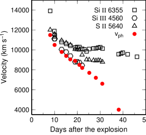
Figure 1: Line velocities measured in the observed spectra (open symbols, Stanishev et al. 2007) compared with the photospheric velocities derived from the spectral modelling (filled red circles). The photospheric velocity follows the Si III line velocity until $\sim 20$ days after the explosion (around maximum).

3.1 Pre-Maximum Epochs

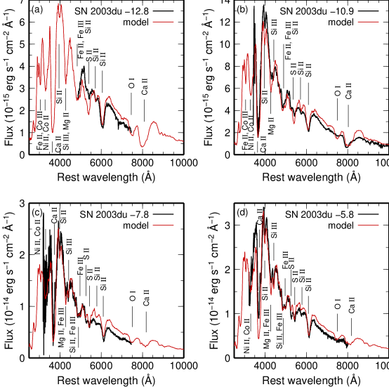
Figure 2: The observed spectra of SN 2003du at the pre-maximum epochs (black) compared with the synthetic spectra (red). Panels (a) - (d) show the spectra at $-12.8$, $-10.9$, $-7.8$ and $-5.8$ days from $B$ maximum, respectively. Line identifications shown in the figures are made only for the major contributions. The synthetic spectra are reddened with $E(B-V)=0.01$ mag.

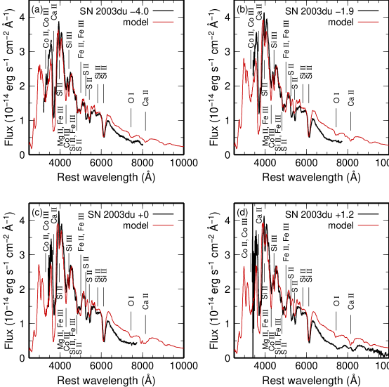
Figure 3: Same as Fig. 2 but at the maximum epochs. Panels (a) - (d) show the spectra at $-4.0$, $-1.9$, $0$ and $+1.2$ days from $B$ maximum, respectively.

In Fig. 2, the observed spectra at epochs from $-12.8$ to $-5.8$ days since $B$ maximum (black) are compared to the synthetic spectra (red). The observed spectra at these epochs show a relatively well defined pseudo-continuum and P Cygni profiles of IMEs and Fe-group elements. At these epochs, the photospheric velocity decreases from 11500 to 9400  km s^-1.

Fe-group elements: The presence of the Fe, Co and Ni lines clearly indicates that some amount of these Fe-group elements are located in the outer layers. Especially, since only a small amount of ⁵⁶Ni has decayed into Fe at such early epochs, the presence of Fe lines requires stable Fe in the outer layers (Tanaka et al. 2008). The mass fraction of stable Fe is found to be $X$(Fe) $\sim 0.003$ - $0.005$.

Calcium: In the spectrum at $-10.9$ days from $B$ maximum, the Ca ii lines near 4000 Å (Ca ii H&K) and 8000 Å (Ca ii IR triplet) show an extremely high velocity ($v\sim 25000$  km s^-1). The origin of this line has been discussed, including the interaction with the circumstellar matter (CSM) or high velocity blobs (e.g.,  Hatano et al. 1999; Thomas et al. 2004; Gerardy et al. 2004; Mazzali et al. 2005b, a; Quimby et al. 2006; Tanaka et al. 2006; Altavilla et al. 2007; Garavini et al. 2007). In this paper, we do not consider the density enhancement with respect to the W7 model. Keeping the W7 density structure, a mass fraction as high as $X$(Ca) $>0.3$ is required at $v>22000$ km s^-1.

The density at the high velocity layers at $v>22000$  km s^-1 in delayed detonation models is higher than in the W7 model by a factor of $\sim 10$ (see e.g., Fig. 11 of Baron et al. 2006). Tanaka et al. (2008) studied the influence of the density structure at the outermost layers. They found that the required mass fraction of Ca is decreased by a factor of $\sim 10$ in the delayed detonation models, but it is still higher than solar abundance (see their Table 3). The density enhancement may also possibly be caused by interaction with the CSM (Gerardy et al. 2004; Mazzali et al. 2005b).

Magnesium, Silicon, and Sulphur: Since the strongest Mg feature at 4200 Å is contaminated by Fe lines, the mass fraction of Mg is not as well constrained as those of Si, S, and Ca. If we assume that the Fe abundance is constrained from the features around 4700 Å, and we attribute any differences to Mg, the mass fraction of Mg is $X$(Mg) $\sim 0.01-0.1$ at $v>9400$  km s^-1.

SN 2003du has relatively narrow Si ii lines. To reproduce the profile of the Si ii $\lambda$6355 line, the mass fraction of Si is required to be $X$(Si) $\sim 0.3$. The dominant element in the layers at $v>13000$  km s^-1 is not Si, but more likely O. The distribution of Si is discussed in Appendix B.

The mass fraction of S is $X$(S) $=0.1-0.2$ around $v=10000$  km s^-1. Although the synthetic spectra for the two earliest epochs show stronger lines than the observations, the later spectra are nicely reproduced.

Carbon and Oxygen: There is no clear C line in the observed spectra except for the possible C ii $\lambda$6578 line at the emission peak of the strongest Si ii $\lambda$6355 line (Stanishev et al. 2007). We derive an upper limit for the C mass as $M$(C) $<$ 0.016 $M_{\odot}$ at $v>10500$  km s^-1 (details are presented in Appendix C). The small mass fraction and mass of C are consistent with the results of previous works (Marion et al. 2006; Thomas et al. 2007; Tanaka et al. 2008; Marion et al. 2009).

The synthetic spectra show a clear O i $\lambda$7774 line around 7500 Å while the presence of such a strong O line is not that clear in the observed spectra. Although the abundance of O is not well constrained, considering the lower abundance of C, Mg, Si and S (see above), we conclude that the dominant element in the outer layers is O. The mass fraction of O at $v>9400$  km s^-1 is $X$(O) $=0.05-0.85$, increasing towards the outer layers.

3.2 Maximum Epochs

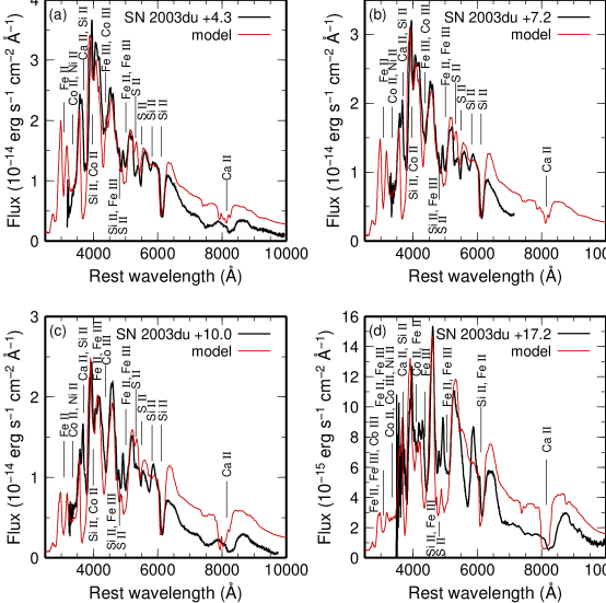
Figure 4: Same as Fig. 2 but at the post-maximum epochs. Panels (a) - (d) show the spectra at $+4.3$, $+7.2$, $+10.0$ and $+17.2$ days from $B$ maximum, respectively.

In Fig. 3, the observed spectra at the epochs from $-4$ to $+1.2$ days since $B$ maximum (black) are compared to the synthetic spectra (red). The element features present in the observed spectra are similar to those in the pre-maximum spectra. At these epochs, the photospheric velocity decreases from 9050 to 8200  km s^-1. The flux of the synthetic spectra at the line-free region at $\lambda>6500$ Å tends to be overestimated because of our assumption of blackbody emission (see Appendix A.1).

Fe-group elements: Around maximum, lines of Fe-group elements are present, as in the pre-maximum epoch. A larger amount of ⁵⁶Ni is required compared with the pre-maximum epochs to block the emission in the near-UV more effectively. The mass fraction of ⁵⁶Ni is $X$(⁵⁶Ni) $=0.5-0.7$ at $v=8200-9050$  km s^-1.

At maximum epochs, the presence of Fe lines does not directly indicate the presence of stable Fe because of the high abundance of the decay product of ⁵⁶Ni. At $B$ maximum ($t_{\rm exp}=20.9$ days), about 10 % of ⁵⁶Ni has already decayed into Fe, and thus an Fe abundance of $\sim 0.05-0.07$ is the product of the decay of ⁵⁶Ni. This is much larger than the abundance of stable Fe required for the pre-maximum spectra, and thus we cannot distinguish the contribution of stable Fe.

Silicon and Sulphur: The Si ii $\lambda$6355 line becomes narrower. The Si distribution at the outer layers derived from the line profile in the pre-maximum spectra (Appendix B) nicely reproduce the maximum spectra. In the spectrum at maximum, the line ratio of two Si ii lines ($\lambda$5972 and 6355, $\mathcal{R}$(Si ii) in Nugent et al. 1995) is also nicely reproduced, suggesting the estimates of the temperature and of the ionization are reasonable (Table 1, Hachinger et al. 2008).

The S ii lines around 5500 Å are also reproduced nicely. Although the photospheric velocity at this epoch is $v_{\rm ph}$$=8200-9050$  km s^-1, the S ii lines, as well as the Si ii lines, are mainly formed at $v\sim 10000$  km s^-1 (see Fig. 1). The “detachment” of the lines is caused by the ionization effect, e.g., S iii is dominant near the photosphere while the fraction of S ii increases towards higher velocities (see Fig. 9 of Tanaka et al. 2008).

3.3 Post-Maximum Epochs

In Fig. 4, the observed spectra at epochs from $+4.3$ to $+17.2$ days since $B$ maximum are compared to the synthetic spectra. At these epochs, the contribution from Fe-group elements is larger than at earlier epochs. The assumption of blackbody emission becomes unreliable, and results in an increasing overestimation of the flux at $\lambda>6500$ Å. Although the photospheric velocity decreases from 7700 to 4000  km s^-1 in our models (Table 1), these values are therefore not strongly constrained.

Since the assumption that there is no energy deposition above the photosphere is also unlikely to hold at this epoch, we use the abundance distribution derived from the modelling of the nebular spectrum (Section 4), rather than optimize the abundances using the spectra at post-maximum epochs. Even with this treatment, the synthetic spectra give reasonable agreement with the observed spectra.

Fe-group elements: The ⁵⁶Ni distribution derived from the nebular spectrum reproduces the Ni, Co and Fe lines present in the observed spectra. The Ni ii, Co ii and Fe ii lines are responsible for the strong blocking of the UV flux. The layers below 8200  km s^-1 down to 4000  km s^-1 (the photospheric velocity of the last spectrum, Fig 4d) are rich in ⁵⁶Ni, which has a mass fraction of $X$(⁵⁶Ni)=$0.7-0.8$. Note that the Fe lines at $4500-5000$ Å in the synthetic spectrum at $t=+17.2$ days are too strong. The discrepancy is also seen in the model for SN 2004eo (Paper I), and it may result from our assumption of no energy deposition in the atmosphere (see above).

Sodium, Silicon, Sulphur, and Calcium: In the last spectrum (Fig. 4d), there is a strong absorption at 5600 Å in the observed spectrum, which is expected to be the Na i D line. With our code, however, this line is not reproduced even if we set $X$(Na) =0.1. This is already too high compared with the prediction by the explosion models: the yield of Na is only $\sim 10^{-5}-10^{-4}M_{\odot}$ (e.g.,  Iwamoto et al. 1999). This is the result of the overestimate of Na ionization by our Monte Carlo code, which is a problem also for other NLTE codes (Mazzali et al. 1997, and references therein), and it may be caused by inaccuracies in the atomic data. Thus, we do not discuss total mass of Na in the following section (Section 6).

The strong Si ii and S ii lines are reproduced well in the spectra at $+4.3$ and $+7.2$ days from $B$ maximum (Fig. 4a and 4b). These lines are formed in layers detached from the photosphere (see Fig. 1) because of the high mass fractions of Si and S, and the large fraction of Si ii and S ii in layers above the photosphere.

The Ca ii H&K and IR triplet lines in the synthetic spectra show too strong high velocity component. They are caused by the high abundance at $v>15000$  km s^-1 derived from the earliest spectra. We believe that the constraints from the earlier spectra are more reliable because the validity of the assumptions in the atmosphere is more certain at those epochs.

4 Nebular-Phase Spectra

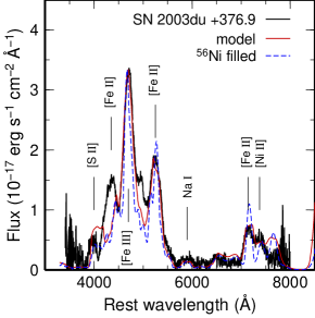
Figure 5: The nebular spectrum of SN 2003du ($+376.9$ days from $B$ maximum, black line, Stanishev et al. 2007) compared with the synthetic spectra (color lines). The red solid line shows the best fit model while the blue dashed line shows the model without central region devoid of ⁵⁶Ni.

A spectrum at $+376.9$ days since $B$ maximum (Stanishev et al. 2007) is modelled to derive the abundances in the deepest layers. A ⁵⁶Ni distribution with a decreasing mass fraction toward higher velocities ($v\mathrel{\hbox to0.0pt{\lower 4.0pt\hbox{\hskip 1.0pt$\sim$}\hss}\raise 1.0pt\hbox{$>$}}10000$  km s^-1) nicely fits the profile of the two strongest Fe lines (red line in Figure 5). This is consistent with the constraints from the spectra at the pre-maximum and maximum epochs.

The innermost layers are dominated by stable Fe. In particular, stable Fe and Ni dominate the abundance at velocities inside of about 3000  km s^-1, accounting for a total mass of $\sim 0.2M_{\odot}$. Most of this is actually stable Fe. Limits to the stable Ni mass can be set by the weakness of the [Ni ii] emission near 7400 Å. As for stable Fe, this is required in the innermost regions in order to keep an ionization balance between Fe ii and Fe iii which allows the shape of the two strong, Fe-dominated emissions at $4500-5000$ Å to be reproduced, as well as their ratio. The bluer emission, near 4600 Å, is in fact dominated by Fe iii, while the redder one, near 5200 Å, is dominated by Fe ii.

If a central region devoid of ⁵⁶Ni is absent (blue dashed line), both Fe features look very sharp, unlike the observations. In order to reduce the flux, the ⁵⁶Ni distribution must be limited to a smaller region, and the overall higher density of the inner region leads to a lower Fe ionization, so that the ratio of the two Fe lines in the blue is no longer correct: the Fe ii-dominated line (near 5200 Å) becomes too strong, as shown in the model in blue dashed line in Figure 5. On the other hand, the presence of stable Fe acts as a coolant, keeping the ionization degree to a level which yields reasonable line intensities (red line).

5 Bolometric Light Curve

The derived abundance distribution is tested against the bolometric LC (Stanishev et al. 2007). SN 2003du is an extremely well-observed SN, and the bolometric LC was constructed with a small uncertainty, including the contribution of the NIR (Stanishev et al. 2007).

For the modelling, we use a Monte Carlo LC code based on that developed in Cappellaro et al. (1997). The code follows the emission and propagation of $\gamma$-rays and positrons from ⁵⁶Ni and ⁵⁶Co decay. Both $\gamma$-rays and positrons are treated with an effective opacity (i.e., the positrons are not assumed to deposit in situ). The opacities adopted are 0.027 cm² gm^-1 for the $\gamma$-rays and 7 cm² gm^-1 for the positrons (Axelrod 1980). For optical opacity, we use an analytic formula introduced by Mazzali et al. (2001a, 2007), which includes the composition dependence (Fe-group elements and other elements) and a time dependence (Hoeflich & Khokhlov 1996).

Fig. 6 shows the comparison between the observed bolometric LC (black squares) and the computed LC (blue line). The input luminosities for the photospheric-phase spectra are also plotted (red circles). The model LC matches well with the observed LC from before maximum until $>1$ year. This suggests that the derived abundance distribution, especially that of ⁵⁶Ni, is reasonable. The bolometric LC derived from the synthetic spectra at epochs after maximum deviate progressively from the observational points, reflecting the increased production of spurious flux redwards of 6500 Å in the synthetic spectra (see Sect. 4).

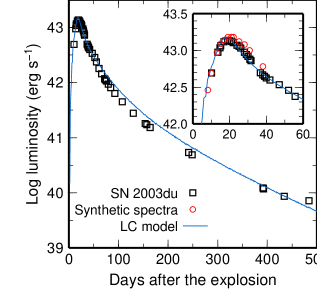
Figure 6: Bolometric LC of SN 2003du (black squares, Stanishev et al. 2007) compared with the bolometric LC model (thin line) and the input bolometric luminosities in the spectral modelling (red circles).

6 Abundance Distribution and Integrated Yields

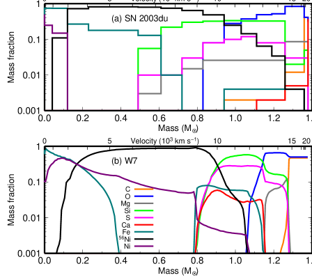
Figure 7: Abundance distribution in the mass coordinate derived from the spectral modelling (a) compared with that of W7 (b). “⁵⁶Ni” represents the mass fraction of ⁵⁶Ni at $t_{\rm exp}=0$ and “Fe” and “Ni” only represent mass fractions of stable Fe and stable Ni, respectively.

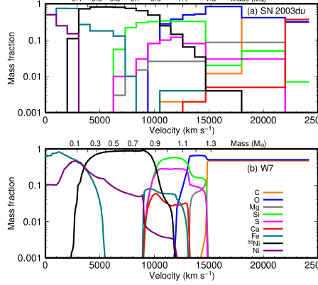
Figure 8: Same as Fig. 7 but in the velocity coordinate.

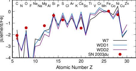
Figure 9: Abundance ratios, i.e., $[{\rm Element/Fe}]={\rm log}_{10}[M/M({\rm Fe})]-{\rm log}_{10}[X/X({\rm Fe})]_{\odot}$ of SN 2003du (red circles), W7 (black line, Nomoto et al. 1984), WDD1 (blue line, Iwamoto et al. 1999), and WDD2 (purple line, Iwamoto et al. 1999). Note that, in this figure, the yields after the radioactive decay are shown, i.e., Fe includes both of stable Fe and the decay product of ⁵⁶Ni, and Ni includes only stable Ni.

6.1 Abundance Distribution

The abundance distribution derived from the modelling of the photospheric- and nebular-phase spectra is shown in Figs. 7 and 8. These two figures show the mass fraction of each element as a function of mass and velocity, respectively. For comparison, the abundance distribution of a deflagration model (W7, Nomoto et al. 1984) is also shown (Figs 7b and 8b). Note the line with “⁵⁶Ni” represents the mass fraction of radioactive ⁵⁶Ni at the time of the explosion ($t_{\rm exp}=0$), and that “Fe” and “Ni” denotes only stable elements.

At the innermost layers ($M_{r}<0.1M_{\odot}$, $v<3000$  km s^-1), stable Fe dominates (Section 4). This is also suggested by the NIR spectrum at late phase (Höflich et al. 2004; Motohara et al. 2006). The existence of stable elements at the innermost layers is consistent with the explosion model. These elements are synthesized via electron capture reactions at high densities, and thus are typically located in the innermost layers.

Above the layer of stable elements, there is a ⁵⁶Ni -dominated layer ($M_{r}=0.1-0.9M_{\odot}$, $v=3000-10000$  km s^-1). This is fairly consistent with the distribution of W7. However, in SN 2003du a moderate amount of ⁵⁶Ni is distributed also in the outer layers, which is important for the blocking of UV light in the early spectra. This was also true for SN 2002bo (Paper I). At $M_{r}>0.9M_{\odot}$ ($v>10000$  km s^-1), there is $\sim 0.01M_{\odot}$ of ⁵⁶Ni.

The layers dominated by Si and S are located above the ⁵⁶Ni -rich layers. Compared with W7, Si has a broader distribution in the mass/velocity coordinates. The moderate amount of Si in the ⁵⁶Ni -rich layers is required to explain the Si absorption line in the spectra after maximum. Even at the outer layers at $v>15000$  km s^-1 ($M_{r}>1.3M_{\odot}$), $X$(Si) $=0.01-0.1$ is also required (Appendix B). This is in contrast to the W7 deflagration model, where C+O remain unburned at $v\mathrel{\hbox to0.0pt{\lower 4.0pt\hbox{\hskip 1.0pt$\sim$}\hss}\raise 1.0pt\hbox{$>$}}15000$  km s^-1.

Above the Si and S-rich layers, the dominant element is O ($M_{r}>1.1M_{\odot}$, $v>13000$  km s^-1). Although this is not directly constrained, a high abundance of Si would not be consistent with the observed line profile (Appendix B) and the mass fractions of C, Mg, S, and Ca are also not larger than O.

The mass of unburned C is quite small, $M$(C) $<0.016M_{\odot}$ at $v>10500$  km s^-1(Appendix C). The small C mass indicates that the progenitor C+O WD was almost completely burned. In the outermost layers ($M_{r}>1.3M_{\odot}$, $v>15000$  km s^-1) only C-burning occurs, and elements heavier than O are not synthesized effectively. Note that there is no constraint on C above $v=18000$  km s^-1, and a mass fraction as high as $X({\rm C})=0.5$ can be allowed. (see Appendix C).

It is also possible that the C abundance in the outermost layers of the progenitor WD is already suppressed in the pre-SN stage. In the single-degenerate scenario, the WD grows by mass accretion from a companion star. In the case of weak He flashes, their nucleosynthesis products can accrete onto the WD. Since the products of the He flashes are not always C and O but could also be heavier elements (e.g.,  Hashimoto et al. 1983), the outermost layers of the WD do not necessarily consist only of nearly equal mass fractions of C and O. The heavier elements synthesized in the pre-SN stage can also be responsible for the high velocity features of the Si and Ca lines present in the earliest spectra (Tanaka et al. 2008).

The overall abundance distribution is not consistent with the almost fully mixed distribution seen in three-dimensional deflagration models (Travaglio et al. 2004; Röpke & Hillebrandt 2005). But the boundaries between stable Fe/⁵⁶Ni, ⁵⁶Ni/IME, IME/O-rich layers are less clear than in the one-dimensional models. This requires moderate degree of mixing during the explosion (Woosley et al. 2007).

The sensitivity of the results on the parameters has been studied in Paper II. In the photospheric phase, the synthetic spectra are sensitive to the velocity at the inner boundary and the element mass fractions. Variations in the mass fractions of up to 25 % are possible, while the synthetic spectra are more sensitive to variations of the velocity: a change of more than 15% can noticeably affect the fits (see Paper II). In the nebular phase, no given inner boundary is required and the constraints on the mass fractions are less uncertain.

Except for the elements shown in Figures 7 and 8, there must be some amount of Ti and Cr in the ejecta. For photospheric-phase spectra, these elements are responsible for the features or the flux level around $3000-3500$ Å. The mass fraction of the sum of Ti and Cr is about $0.001-0.01$ (Papers I and II). However, since this wavelength range is not covered in most spectra used in this paper, we refrain from discussing the distribution and total yields of these elements.

6.2 Integrated Yields

Table 2: The total mass of the elements in SN 2003du derived from spectral modelling and nucleosynthesis products of different SN Ia explosion models

Species	SN 2003du	W71	WDD12	WDD22	b30_3d_7683	Y124	O-DDT5
C	$<$1.6E-02∗	4.83E-02	5.42E-03	8.99E-03	2.78E-01	8.73E-03	3.49E-03
O	2.3E-01	1.43E-01	8.82E-02	6.58E-02	3.39E-01	1.07E-01	1.51E-01
Na	—∗∗	6.32E-05	8.77E-05	2.61E-05	8.65E-04	—∗∗∗	5.87E-05
Mg	2.4E-02	8.58E-03	7.69E-03	4.52E-03	8.22E-03	8.70E-2	2.16E-02
Si	2.1E-01	1.57E-01	2.74E-01	2.07E-01	5.53E-02	1.27E-1	2.87E-01
S	4.8E-02	8.70E-02	1.63E-01	1.24E-01	2.74E-02	7.03E-2	1.27E-01
Ca	1.4E-03	1.19E-02	3.10E-02	2.43E-02	3.61E-03	1.82E-2	1.70E-02
Ti	—∗∗	3.43E-04	1.13E-03	1.02E-03	8.98E-05	1.41E-5	8.72E-04
Cr	—∗∗	8.48E-03	2.05E-02	1.70E-02	3.19E-03	2.96E-4	1.04E-02
Fea	1.8E-01	1.63E-01	1.08E-01	1.02E-01	1.13E-01	6.50E-3b	1.11E-01
56Ni	6.5E-01	5.86E-01	5.64E-01	6.90E-01	4.18E-01	9.26E-1c	5.40E-01
Nid	2.4E-02	1.26E-01	3.82E-02	5.87E-02	1.06E-01	—∗∗∗	8.05E-02

^∗Upper limit at $v>10500$  km s^-1. ^∗∗Not constrained. ^∗∗∗Not given.
^aStable isotopes except for ⁵⁶Fe from ⁵⁶Co decay.
^bOnly ⁵²Fe.
^cThe sum of Fe-group elements except for ⁵²Fe, and thus, the upper limit for ⁵⁶Ni (see Plewa 2007).
^dStable isotopes ⁵⁸Ni, ⁶⁰Ni, ⁶¹Ni, ⁶²Ni, and ⁶⁴Ni.
${}^{1}\,$Nomoto et al. (1984), ${}^{2}\,$Iwamoto et al. (1999), ${}^{3}\,$Travaglio et al. (2004), ${}^{4}\,$Plewa (2007), ${}^{5}\,$Maeda et al. (2010b)

The ejected mass of each element in SN 2003du was calculated by integrating the abundance distribution assuming the W7 density structure. Results are summarized in Table 2. For comparison, the nucleosynthetic yields of the following models are also shown: one-dimensional deflagration model (W7, Nomoto et al. 1984), one-dimensional delayed detonation models (WDD1 and WDD2 , Iwamoto et al. 1999), three-dimensional deflagration model (b30_3d_768, Travaglio et al. 2004), two-dimensional detonating failed deflagration model (Y12, Plewa 2007), and two-dimensional off-center delayed detonation model (O-DDT, Maeda et al. 2010b).

In Figure 9, the derived yields are compared with those of the one-dimensional models in the abundance ratio to Fe, normalized by the solar abundances, i.e., $[{\rm Element/Fe}]={\rm log}_{10}[M/M({\rm Fe})]-{\rm log}_{10}[X/X({\rm Fe})]_{\odot}$. Here, the yields after the radioactive decays are shown, i.e., Fe means the sum of stable Fe and the decay product of ⁵⁶Ni, and Ni includes only stable Ni.

In SN 2003du, the ejected mass of neutron-rich elements is estimated to be $\sim 0.2M_{\odot}$. They are synthesized by electron capture reactions and mostly distributed in the innermost layers. The mass of ⁵⁶Ni is $0.65M_{\odot}$, which is the largest among all synthesized elements. The mass of IMEs (Mg, Si, S, and Ca) is $\sim 0.28M_{\odot}$ in total. The mass of O is estimated to be $0.23M_{\odot}$, and is predominantly located in the outer layers. There is no sign of C, and the upper limit is $M$(C) $<0.016M_{\odot}$ at $v>10500$  km s^-1.

From these yields, the validity of the W7 density structure can be tested. We use the formula for the kinetic energy of SNe Ia: $E_{K}=[1.56M({\rm{}^{56}Ni})+1.74M({\rm stable\ Fe})+1.24M({\rm IME})-0.46]\times 10^{51}$ erg (Woosley et al. 2007), where $M$(⁵⁶Ni), $M$(stable Fe) and $M$(IME) are the ejected mass of ⁵⁶Ni, stable Fe-group elements and the IMEs, respectively. Substituting the element masses derived for SN 2003du, we derive an ejecta kinetic energy of $E_{K}=1.25\times 10^{51}$ erg, which is in a good agreement with the kinetic energy of the W7 model ($E_{K}\sim 1.3\times 10^{51}$). Thus, the element masses derived from the modelling under the assumption of the W7 density structure are self-consistent.

We first compare the integrated yields with those of one-dimensional models (Table 2). The total mass of stable Fe-group elements estimated for SN 2003du is reasonably consistent with that of the one-dimensional explosion models. The amount of neutron-rich stable elements in the central region is sensitive to the deflagration speed, which affects the efficiency of the electron captures. Thus, the good agreement implies that the deflagration speed in the explosion models is reasonable.

The mass of ⁵⁶Ni in SN 2003du is also consistent with that of the one-dimensional deflagration and delayed detonation models. In the delayed detonation models, a larger amount of ⁵⁶Ni suggests an earlier transition to a detonation. Thus, if the delayed detonation model is the correct scenario, a transition density close to that of the models WDD1 and WDD2 is reasonable for SN 2003du.

The total mass of IMEs estimated for SN 2003du is smaller than in the delayed detonation models, while the mass of O in SN 2003du is larger. This suggests that O burning in SN 2003du was not as strong as in the delayed detonation models. However, the unburned C mass in the outermost layers in SN 2003du is smaller than in the deflagration models. Thus, the outermost part of the C+O WD is burned more intensely than in the deflagration model (see also Section 6.1).

Next, we compare the results with multi-dimensional models. The mass of ⁵⁶Ni in SN 2003du is clearly larger than in the three-dimensional deflagration model (Travaglio et al. 2004). The three-dimensional deflagration model also predicts more unburned C, which is not consistent with the small C mass derived for SN 2003du. Thus, also from the nucleosynthetic point of view, the three-dimensional deflagration model is unlikely to be a reasonable model for a normal SNe Ia such as SN 2003du.

It is interesting to compare the yields with the detonating failed deflagration model (Plewa 2007) and the off-center delayed detonation model (Maeda et al. 2010b), because these models may explain the kinematic offset in the central region suggested by the NIR spectra at late phases (Höflich et al. 2004; Motohara et al. 2006; Maeda et al. 2010c). The detonating failed deflagration model (Plewa 2007) predicts too much ⁵⁶Ni compared with SN 2003du. Thus, this model does not seem a likely model for normal SNe Ia, as already cautioned by Meakin et al. (2009). The yields of the two-dimensional off-center delayed detonation model (Maeda et al. 2010b) are in good agreement with those derived for SN 2003du. It is, however, noted that the model predicts ⁵⁶Ni synthesized near the center, while the existence of a region free of ⁵⁶Ni is suggested from our one-dimensional analysis of the nebular phase spectrum (Section 4).

6.3 Comparison with SNe 2002bo and 2004eo

In this section, we compare the abundance distributions and integrated yields derived for SN 2003du with those derived for SNe 2002bo (Paper I) and 2004eo (Paper II). SN 2002bo is a normally luminous SN ($\Delta m_{15}=1.13$ mag), but has high line velocities and a high velocity gradient at early phases (Benetti et al. 2004). SN 2004eo has a transitional luminosity between normal and subluminous SNe Ia, with a relatively rapid decline of the light curve ($\Delta m_{15}=1.46$ mag, Pastorello et al. 2007).

These three SNe have in common an innermost layer of stable Fe-group elements which are synthesized by electron capture. The mass of this region $\sim 0.2M_{\odot}$ is similar in the three SNe studied thus far (see also Mazzali et al. 2007), although the mass of ⁵⁶Ni is different, 0.65, 0.52, and 0.43 $M_{\odot}$ for SNe 2003du, 2002bo, and 2004eo, respectively.

The most significant difference between SNe 2003du and 2002bo is in the outermost layers. In SN 2002bo Si reaches the outer layers (Paper I). The abundance of Si in the outer layers of SN 2002bo is larger than in SN 2003du. This is the primary reason why Si line velocities in SN 2002bo are higher than in SN 2003du, as demonstrated in Appendix B. Tanaka et al. (2008) also suggested that the difference between high-velocity and low-velocity SNe Ia is caused by the difference in the Si abundance.

Alternatively, the difference can also be caused by the difference in the density structure in the outer layers. Maeda et al. (2010a) pointed that the difference in the velocity (and/or velocity gradient) is caused by viewing-angle effects in an aspherical explosion that has different density structures depending on the viewing angle.

SN 2002bo also has a more extended ⁵⁶Ni distribution than in SN 2003du. This explains the rapid rise of the LC of SN 2002bo (Paper I). Pignata et al. (2008) suggest that the rising time of the LC of SNe with a high velocity gradient is generally shorter than that of SNe with a low velocity gradient. Thus, the extended ⁵⁶Ni distribution may be a common property of high-velocity SNe.

Interestingly, SNe 2003du and 2004eo have a similar distribution of Si, O, and C above $v=10000$  km s^-1 ($M_{r}=0.9M_{\odot}$). This indicates that the different shapes of the LCs of these two SNe result from the difference in the inner layers. In fact, a difference between these SNe is seen in the mass and mass fraction of ⁵⁶Ni. A smaller amount of ⁵⁶Ni is responsible for the fainter luminosity and more rapid decline of SN 2004eo (see also Paper II).

7 Conclusions

We have studied the element abundance distribution in SN 2003du by modelling the optical spectra at the photospheric and nebular phases. These are used to place constraints on the abundances at the outer and inner layers, respectively. Since SN 2003du is a normal Type Ia SN, both photometrically and spectroscopically, the abundance distribution derived for SN 2003du can be considered as representative of normal Type Ia SNe.

The abundance distribution and the integrated yields in SN 2003du can be summarized as follows. The innermost layers are dominated by stable, neutron-rich elements, with a total mass of $\sim 0.2M_{\odot}$. The yield is roughly consistent with the results of one-dimensional models. This may imply that the deflagration speed assumed in the models is reasonable.

Above the stable elements, there is a thick ⁵⁶Ni-rich layer. The total mass of ⁵⁶Ni is $0.65M_{\odot}$, which is consistent with the one-dimensional deflagration model and the one-dimensional delayed detonation models with transition density $\sim 1-2\times 10^{7}\ {\rm g\ cm^{-3}}$. The ⁵⁶Ni mass is larger than in the three-dimensional deflagration model and smaller than in the detonating failed deflagration model.

The layers dominated by Si and S are located above the ⁵⁶Ni -rich layers. The dominant element at $M_{r}>1.1M_{\odot}$ ($v>13000$  km s^-1) is O. The progenitor C+O WD is almost entirely burned, and the mass of leftover unburned C is quite small ($<0.016M_{\odot}$ at $v>10500$  km s^-1). The small mass of unburned C is consistent with the delayed detonation model. However, the mass of O derived for SN 2003du is larger than that in the delayed detonation model. These results suggest that in the outermost layers C-burning is more intense than in the deflagration model, but O burning is not as strong as in the delayed detonation models.

The boundary between stable Fe/⁵⁶Ni, ⁵⁶Ni/IME, IME/O-rich layers is not as sharp as in the one-dimensional models, suggesting a moderate degree of mixing. However, the strong mixing seen in the multi-dimensional deflagration model is not preferable.

This work has made use of the SUSPECT supernova spectral archive. V.S. is financially supported by FCT Portugal under program Ciência 2008. This research has been supported in part by World Premier International Research Center Initiative, MEXT, Japan.

Appendix A Assumptions in the Code

A.1 Photospheric Phase

The spectrum synthesis code for the photospheric phases assumes a sharply defined spherical photosphere as an inner boundary. At the inner boundary, blackbody radiation is assumed. Since the temperature structure [$T_{R}(r)$] is unknown at first, the calculation starts with an assumed temperature. Using this temperature, the ionization and excitation in the optically thin atmosphere above the photosphere are calculated considering the dilution of the radiation. The degree of dilution $W$ is defined by the equation $J=WB(T_{R})$ in our code.

The excitation (the population of an excited level $n_{j}$; $j=1$ for the ground state) is computed as in Abbott & Lucy (1985) and Lucy (1999):

$$\frac{n_{j}}{n_{1}}=W\frac{g_{j}}{g_{1}}e^{-\epsilon_{j}/k_{B}T_{R}},$$ (1)

where $g_{j}$ and $\epsilon_{j}$ are the statistical weight and the excitation energy from the ground level, respectively.

For the ionization, the nebular approximation, which is similar to that made in the studies of stellar winds (Lucy & Solomon 1970; Abbott & Lucy 1985) or planetary nebulae (Gurzadyan 1997), are adopted with the modifications for SNe (Mazzali & Lucy 1993):

$$\frac{N_{i+1}N_{e}}{N_{i}}=[\delta\zeta+(1-\zeta)W]W\left(\frac{T_{e}}{T_{R}}\right)^{1/2}\left(\frac{N_{i+1}N_{e}}{N_{i}}\right)^{*}_{T_{R}},$$ (2)

where $N_{e}$ and $T_{e}$ are the electron density and the electron temperature, respectively. In the equation, $\delta$ and $\zeta$ are the correction factors for the optically thick continuum shorter than the Ca ii ionization edge and the fraction of recombinations that go directly to the ground state, respectively (Mazzali & Lucy 1993). The first and second terms in the first square brackets on the right hand side represents the excitation from the ground and excited levels, respectively. The last term on the right hand side is the ionization computed from the Saha equation with $T_{R}$. For the electron temperature, $T_{e}=0.9T_{R}$ is crudely assumed (Klein & Castor 1978; Abbott & Lucy 1985).

With the ionization and excitation states, line optical depths are calculated under the Sobolev approximation, which is a sound approximation in rapidly expanding envelope with large velocity gradients (Castor 1970; Lucy 1971). A number of photon packets are traced above the photosphere in spherical coordinates, taking into account electron scattering and line scattering. For line scattering, the effect of the line branching is included (Lucy 1999; Mazzali 2000; Pinto & Eastman 2000). The stream of the photon packets gives the flux at each radial mesh and a frequency moment is calculated by

$$\bar{\nu}=\frac{\int\nu J_{\nu}d\nu}{\int J_{\nu}d\nu}.$$ (3)

The radiation temperature is estimated from this frequency moment via

$$\bar{x}=\frac{h\bar{\nu}}{k_{B}T_{R}}.$$ (4)

Here $\bar{x}$ represents for the mean energy of the blackbody radiation [$\bar{x}=(h/k_{B}T_{R})(\int\nu B_{\nu}d\nu/\int B_{\nu}d\nu)=3.832$].

Using this new temperature structure, the ionization and excitation are updated. Then, the next Monte Carlo ray tracing starts. This procedure is continued until the temperature converges. Finally, the emergent spectrum is calculated using a formal integral (Lucy 1999).

It is known that these assumptions give a good approximation to the results of detailed NLTE calculations (Pauldrach et al. 1996). However, since no energy deposition by ⁵⁶Ni and ⁵⁶Co is assumed above the photosphere, the assumptions become unreliable as a large part of the ⁵⁶Ni-rich layer becomes optically thin. In addition, the assumption of a sharp photosphere becomes progressively invalid after maximum brightness. Thus, the quantities derived by fitting the spectra at later epochs (especially after maximum brightness in SNe Ia) are more uncertain.

A.2 Nebular Phase

The spectrum synthesis code for the nebular phases first calculates the energy deposition by $\gamma$-rays and positrons produced in the decay of ⁵⁶Co. For a given distribution of ⁵⁶Ni, the energy deposition in each shell is evaluated in a Monte Carlo scheme (Cappellaro et al. 1997). The deposited energy is spent in the ionization and in the heating of thermal electrons. The latter is known to be dominant in Fe-rich ejecta ($\sim 97$ per cent, Axelrod 1980).

For given ionization fractions in the ejecta, the heating of the thermal electrons ($\Gamma$) is balanced with the radiative cooling (thermal balance):

$$\Gamma=\Gamma_{\rm line}+\Gamma_{\rm ff}+\Gamma_{\rm rec},$$ (5)

where $\Gamma_{\rm line}$, $\Gamma_{\rm ff}$ and $\Gamma_{\rm rec}$ are the cooling via lines, free-free emission, and recombination, respectively. Since the contribution from the latter two are smaller than the line cooling ($\sim 0.03$ and $4$ per cent, respectively, Ruiz-Lapuente & Lucy 1992), we only consider cooling by lines. The line cooling per unit volume by lines is given by

$$\Gamma_{\rm line}=\sum\limits_{k}n_{kj}\sum\limits_{ij}A_{ji}h\nu_{ij}\beta_{ij},$$ (6)

where $n_{kj}$ is the number density of the ion $k$ in the energy state $j$, and $A_{ji}$ and $\beta_{ij}$ represents for the Einstein A-coefficient and the escape probability of the transition $j\rightarrow i$. From this thermal balance, an electron temperature is evaluated in each shell.

The ionization fractions are determined balancing impact ionization by non-thermal electrons and recombinations (ionization balance). Collisional ionization by thermal electrons can be neglected (Ruiz-Lapuente & Lucy 1992). The ionization balance is solved for a given electron temperature. Using this new ionization, the thermal balance is reconsidered, i.e., the temperature and the ionizations are solved iteratively. After the convergence, the emergent spectrum is computed by integrating the contribution from each shell considering the Doppler shift.

Appendix B Silicon Abundance at the Outer Layers

The Si ii line profile in SN 2003du is rather narrow and it is similar to that found in, e.g., SNe 2002er (Fig. 10, HVG, Kotak et al. 2005), 2003cg (LVG, Elias-Rosa et al. 2006), 2005cg (LVG, Quimby et al. 2006). This is in contrast to the broad absorption seen in SNe 2002bo (Fig. 10, HVG, Benetti et al. 2004), 2002dj (HVG, Pignata et al. 2008), 2006X (HVG, Wang et al. 2008; Yamanaka et al. 2009), or a possible boxy profile in SNe 1990N (LVG, Leibundgut et al. 1991), 2001el (LVG, Mattila et al. 2005), 2004dt (HVG, Altavilla et al. 2007), 2005cf (Fig. 10, LVG, Garavini et al. 2007; Wang et al. 2009). Here LVG and HVG mean low velocity gradient and high velocity gradient, respectively. These are the classifications of Type Ia SNe based on the temporal evolution of the Si ii line velocity (Benetti et al. 2005). Note that high velocity features of Ca ii lines are commonly seen in both groups at pre-maximum epochs (Mazzali et al. 2005a).

We use the spectrum at $-10.9$ days from $B$ maximum ($v_{\rm ph}=10500$  km s^-1) to constrain the distribution of Si in the outer layers because this spectrum is reproduced better than the one at $-12.8$ days (Fig. 2). To reproduce the observed profile, a moderately mixed-out Si distribution is required. The mass fraction of Si is $X$(Si)$\sim 0.3$ at $v=10500-15000$  km s^-1 and it is suppressed at the outer layers, $X$(Si)$\sim 0.02-0.05$ at $v>15000$  km s^-1 (see Figs. 7 and 8). This model is shown in Figures 2 and 10 by the red line.

In the right panel of Figure 10, two other models are shown. The orange line (”cutoff”) shows a model spectrum where the Si abundance has been set to $X$(Si)=0 at $v>15000$  km s^-1 as in the W7 model (Fig. 8). In this model, the absorption of Si at $v>15000$  km s^-1 is clearly too weak, suggesting that some degree of burning took place in the outer layers (Gerardy et al. 2004).

The purple line (”homogeneous”) shows the model spectrum with a homogeneous Si abundance with $X$(Si)=0.3 at $v>10500$  km s^-1. In this case, the absorption at a high Doppler shift is too strong. This gives a similar profile to that in SNe 2002bo and 2005cf. In fact, such an extended Si distribution was derived for SN 2002bo in Paper I.

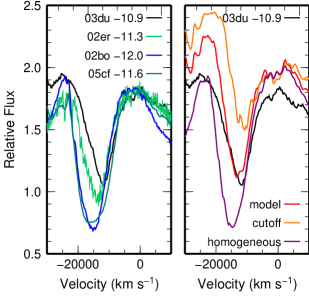
Figure 10: The line profile of the Si ii $\lambda$6355 shown in the Doppler velocity measured from the rest wavelength of the Si II line ($\lambda=6355$ Å). Left: The Si line profile in SNe 2003du (at $-10.9$ days from $B$ maximum, Stanishev et al. 2007), 2002er ($-11.3$ days, Kotak et al. 2005), 2002bo ($-12.0$ days, Benetti et al. 2004), and 2005cf ($-11.6$ days, Garavini et al. 2007) at similar epochs. These spectra are normalized to SN 2003du at $\lambda=6355$ Å. Right: The Si line profile in SN 2003du at $-10.9$ days from $B$ maximum compared with three synthetic spectra. Three model spectra are normalized to the best fit model at $\lambda=6355$ Å. The red line shows the best fit model using the abundance distribution shown in Figs. 7 and 8. The orange line (“cutoff”) shows the model spectrum where the mass fraction of Si, $X$(Si), is set to be zero above 15000  km s^-1. The purple line (“homogeneous”) shows the model spectrum where the homogeneous Si abundance with $X$(Si)=0.3 is assumed at $v>10500$  km s^-1.

Appendix C Upper Limit for the Mass of Unburned Carbon

Lines of carbon are not clearly seen in the optical spectra of SN 2003du. A marginal detection may be seen in correspondence of the emission peak of Si ii $\lambda$6355 (Stanishev et al. 2007; Tanaka et al. 2008). The profile around the emission peak is enlarged in Figure 11 and plotted versus Doppler velocity measured from the C ii $\lambda$6578 line. We use the spectrum at $-10.9$ days from $B$ maximum ($v_{\rm ph}=10500$  km s^-1) to estimate an upper limit for unburned C since the emission peak of the Si line is reproduced more nicely than in the spectrum at $-12.8$ days.

We first divide the ejecta at $v>10500$  km s^-1 into three parts, with boundaries at $v=15000$ and $18000$  km s^-1. At $v>18000$  km s^-1, no constraints can be obtained on the C abundance because of the low density (weakness of the line) and the blending with the strong Si ii line. Thus, we could set the upper limit of C as $X$(C)=0.5 at $v>18000$  km s^-1. In practice, since there are other elements such as Si and Ca in this velocity space, the mass fraction is set to be $X$(C)=0.4 at $v>18000$  km s^-1 in the best fit model. Since the ejecta mass at $v>18000$  km s^-1 is $2.0\times 10^{-2}M_{\odot}$, the upper limit of the C mass at $v>18000$  km s^-1 is $1.0\times 10^{-2}M_{\odot}$.

The model spectrum with $X$(C)$=0.05$ at $v=15000-18000$  km s^-1 shows a noticeable C ii line at the emission peak of the Si ii line (left panel of Fig. 11). Since the ejecta mass at $v=15000-18000$  km s^-1 is $6.0\times 10^{-2}M_{\odot}$, the upper limit of the C mass in this layer is $3\times 10^{-3}M_{\odot}$, which is smaller than the C mass allowed in the outermost layers ($1.0\times 10^{-2}M_{\odot}$ at $v>18000$  km s^-1).

At $v=10500-15000$  km s^-1, the constraint on the C abundance is even stronger. The model spectrum with $X$(C) $=0.008$ gives a clear absorption trough of the C ii line (right panel of Fig. 11). Thus, although the ejecta mass at $v=10500-15000$  km s^-1 is large ($3.4\times 10^{-1}M_{\odot}$), the C mass at these layers is less than $3\times 10^{-3}M_{\odot}$.

Thus, most of the C that is allowed must be located at $v>18000$  km s^-1. Summing up the upper limits to the C mass in different layers, we can safely conclude that the mass of C ejected in SN 2003du is $<1.6\times 10^{-2}M_{\odot}$ at $v>10500$  km s^-1. This is less than in the deflagration models ($4.86\times 10^{-2}M_{\odot}$), where $X$(C)=0.5 at $v\mathrel{\hbox to0.0pt{\lower 4.0pt\hbox{\hskip 1.0pt$\sim$}\hss}\raise 1.0pt\hbox{$>$}}15000$  km s^-1 (see Figs. 7 and 8, and Table 2). Note that all estimates are performed assuming the density structure of W7 model. If a delayed detonation model was used, $X$(C) in the outermost layers would be smaller (Tanaka et al. 2008).

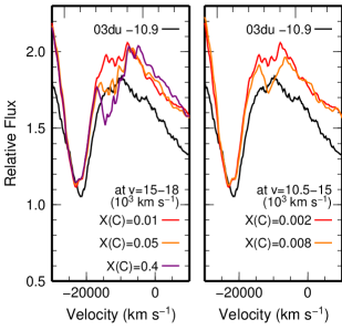
Figure 11: The line profile around the emission peak of the Si ii $\lambda$6355 line shown in the Doppler velocity measured from the C ii $\lambda$6578. Left: The profile in SNe 2003du at $-10.9$ days from $B$ maximum compared with the model spectra with $X$(C)=0.01 (red, best fit), 0.05 (orange), and 0.4 (purple) at $v=15000-18000$  km s^-1. Right: The profile in SN 2003du at $-10.9$ days from $B$ maximum compared with the model spectra with $X$(C)=0.002 (red, best fit) and 0.008 (orange) at $v=10500-15000$  km s^-1.

References

- Abbott & Lucy (1985) Abbott D. C., Lucy L. B., 1985, ApJ, 288, 679
- Altavilla et al. (2007) Altavilla G. et al., 2007, A&A, 475, 585
- Anupama et al. (2005) Anupama G. C., Sahu D. K., Jose J., 2005, A&A, 429, 667
- Axelrod (1980) Axelrod T. S., 1980, PhD thesis, AA(California Univ., Santa Cruz.)
- Baron et al. (2006) Baron, E., Bongard, S., Branch, D., Hauschildt, P. H., 2006, ApJ, 645, 480
- Benetti et al. (2005) Benetti S. et al., 2005, ApJ, 623, 1011
- Benetti et al. (2004) Benetti S. et al., 2004, MNRAS, 348, 261
- Branch et al. (2006) Branch D. et al., 2006, PASP, 118, 560
- Branch et al. (2007) Branch D. et al., 2007, PASP, 119, 709
- Cappellaro et al. (1997) Cappellaro E., Mazzali P. A., Benetti S., Danziger I. J., Turatto M., della Valle M., Patat F., 1997, A&A, 328, 203
- Castor (1970) Castor J. I., 1970, MNRAS, 149, 111
- Elias-Rosa et al. (2006) Elias-Rosa N. et al., 2006, MNRAS, 369, 1880
- Gamezo et al. (2005) Gamezo V. N., Khokhlov A. M., Oran E. S., 2005, ApJ, 623, 337
- Garavini et al. (2007) Garavini G. et al., 2007, A&A, 471, 527
- Gerardy et al. (2004) Gerardy C. L. et al., 2004, ApJ, 607, 391
- Gurzadyan (1997) Gurzadyan G. A., 1997, The Physics and Dynamics of Planetary Nebulae. Springer-Verlag Berlin Heidelberg New York
- Hachinger et al. (2008) Hachinger S., Mazzali P. A., Tanaka M., Hillebrandt W., Benetti S., 2008, MNRAS, 389, 1087
- Hashimoto et al. (1983) Hashimoto M.-A., Hanawa T., Sugimoto D., 1983, PASJ, 35, 1
- Hatano et al. (1999) Hatano K., Branch D., Fisher A., Baron E., Filippenko A. V., 1999, ApJ, 525, 881
- Hillebrandt & Niemeyer (2000) Hillebrandt W., Niemeyer J. C., 2000, ARA&A, 38, 191
- Hoeflich & Khokhlov (1996) Hoeflich P., Khokhlov A., 1996, ApJ, 457, 500
- Höflich et al. (2004) Höflich P., Gerardy C. L., Nomoto K., Motohara K., Fesen R. A., Maeda K., Ohkubo T., Tominaga N., 2004, ApJ, 617, 1258
- Iwamoto et al. (1999) Iwamoto K., Brachwitz F., Nomoto K., Kishimoto N., Umeda H., Hix W. R., Thielemann F.-K., 1999, ApJS, 125, 439
- Jordan et al. (2008) Jordan IV G. C., Fisher R. T., Townsley D. M., Calder A. C., Graziani C., Asida S., Lamb D. Q., Truran J. W., 2008, ApJ, 681, 1448
- Kasen et al. (2009) Kasen D., Röpke F. K., Woosley S. E., 2009, Nature, 460, 869
- Khokhlov (1991) Khokhlov A. M., 1991, A&A, 245, 114
- Klein & Castor (1978) Klein R. I., Castor J. I., 1978, ApJ, 220, 902
- Kotak et al. (2005) Kotak R. et al., 2005, A&A, 436, 1021
- Leibundgut et al. (1991) Leibundgut B., Kirshner R. P., Filippenko A. V., Shields J. C., Foltz C. B., Phillips M. M., Sonneborn G., 1991, ApJ, 371, L23
- Lucy (1971) Lucy L. B., 1971, ApJ, 163, 95
- Lucy (1999) —, 1999, A&A, 345, 211
- Lucy & Solomon (1970) Lucy L. B., Solomon P. M., 1970, ApJ, 159, 879
- Maeda et al. (2010a) Maeda K. et al., 2010a, Nature, 466, 82
- Maeda et al. (2010b) Maeda K., Röpke F. K., Fink M., Hillebrandt W., Travaglio C., Thielemann F., 2010b, ApJ, 712, 624
- Maeda et al. (2010c) Maeda K., Taubenberger S., Sollerman J., Mazzali P. A., Leloudas G., Nomoto K., Motohara K., 2010c, ApJ, 708, 1703
- Marion et al. (2009) Marion G. H., Höflich P., Gerardy C. L., Vacca W. D., Wheeler J. C., Robinson E. L., 2009, AJ, 138, 727
- Marion et al. (2006) Marion G. H., Höflich P., Wheeler J. C., Robinson E. L., Gerardy C. L., Vacca W. D., 2006, ApJ, 645, 1392
- Mattila et al. (2005) Mattila S., Lundqvist P., Sollerman J., Kozma C., Baron E., Fransson C., Leibundgut B., Nomoto K., 2005, A&A, 443, 649
- Mazzali (2000) Mazzali P. A., 2000, A&A, 363, 705
- Mazzali et al. (2005a) Mazzali P. A. et al., 2005a, ApJ, 623, L37
- Mazzali et al. (2005b) Mazzali P. A., Benetti S., Stehle M., Branch D., Deng J., Maeda K., Nomoto K., Hamuy M., 2005b, MNRAS, 357, 200
- Mazzali et al. (1997) Mazzali P. A., Chugai N., Turatto M., Lucy L. B., Danziger I. J., Cappellaro E., della Valle M., Benetti S., 1997, MNRAS, 284, 151
- Mazzali et al. (2000) Mazzali P. A., Iwamoto K., Nomoto K., 2000, ApJ, 545, 407
- Mazzali & Lucy (1993) Mazzali P. A., Lucy L. B., 1993, A&A, 279, 447
- Mazzali et al. (1992) Mazzali P. A., Lucy L. B., Butler K., 1992, A&A, 258, 399
- Mazzali et al. (1993) Mazzali P. A., Lucy L. B., Danziger I. J., Gouiffes C., Cappellaro E., Turatto M., 1993, A&A, 269, 423
- Mazzali et al. (2001a) Mazzali P. A., Nomoto K., Cappellaro E., Nakamura T., Umeda H., Iwamoto K., 2001a, ApJ, 547, 988
- Mazzali et al. (2001b) Mazzali P. A., Nomoto K., Patat F., Maeda K., 2001b, ApJ, 559, 1047
- Mazzali et al. (2007) Mazzali P. A., Röpke F. K., Benetti S., Hillebrandt W., 2007, Science, 315, 825
- Mazzali et al. (2008) Mazzali P. A., Sauer D. N., Pastorello A., Benetti S., Hillebrandt W., 2008, MNRAS, 386, 1897
- Meakin et al. (2009) Meakin C. A., Seitenzahl I., Townsley D., Jordan G. C., Truran J., Lamb D., 2009, ApJ, 693, 1188
- Motohara et al. (2006) Motohara K. et al., 2006, ApJ, 652, L101
- Nomoto et al. (1976) Nomoto K., Sugimoto D., Neo S., 1976, Ap&SS, 39, L37
- Nomoto et al. (1984) Nomoto K., Thielemann F.-K., Yokoi K., 1984, ApJ, 286, 644
- Nomoto et al. (1994) Nomoto K., Yamaoka H., Shigeyama T., Kumagai S., Tsujimoto T., 1994, in Supernovae, Bludman S. A., Mochkovitch R., Zinn-Justin J., eds., p. 199
- Nugent et al. (1995) Nugent P., Phillips M., Baron E., Branch D., Hauschildt P., 1995, ApJ, 455, L147
- Pastorello et al. (2007) Pastorello A. et al., 2007, MNRAS, 377, 1531
- Pauldrach et al. (1996) Pauldrach A. W. A., Duschinger M., Mazzali P. A., Puls J., Lennon M., Miller D. L., 1996, A&A, 312, 525
- Perlmutter et al. (1999) Perlmutter S. et al., 1999, ApJ, 517, 565
- Phillips (1993) Phillips M. M., 1993, ApJ, 413, L105
- Pignata et al. (2008) Pignata G. et al., 2008, MNRAS, 388, 971
- Pinto & Eastman (2000) Pinto P. A., Eastman R. G., 2000, ApJ, 530, 757
- Plewa (2007) Plewa T., 2007, ApJ, 657, 942
- Plewa et al. (2004) Plewa T., Calder A. C., Lamb D. Q., 2004, ApJ, 612, L37
- Quimby et al. (2006) Quimby R., Höflich P., Kannappan S. J., Rykoff E., Rujopakarn W., Akerlof C. W., Gerardy C. L., Wheeler J. C., 2006, ApJ, 636, 400
- Reinecke et al. (2002) Reinecke M., Hillebrandt W., Niemeyer J. C., 2002, A&A, 391, 1167
- Riess et al. (1998) Riess A. G. et al., 1998, AJ, 116, 1009
- Riess et al. (1996) Riess A. G., Press W. H., Kirshner R. P., 1996, ApJ, 473, 88
- Röpke & Hillebrandt (2005) Röpke F. K., Hillebrandt W., 2005, A&A, 431, 635
- Röpke & Niemeyer (2007) Röpke F. K., Niemeyer J. C., 2007, A&A, 464, 683
- Ruiz-Lapuente & Lucy (1992) Ruiz-Lapuente P., Lucy L. B., 1992, ApJ, 400, 127
- Stanishev et al. (2007) Stanishev V. et al., 2007, A&A, 469, 645
- Stehle et al. (2005) Stehle M., Mazzali P. A., Benetti S., Hillebrandt W., 2005, MNRAS, 360, 1231
- Tanaka et al. (2008) Tanaka M. et al., 2008, ApJ, 677, 448
- Tanaka et al. (2006) Tanaka M., Mazzali P. A., Maeda K., Nomoto K., 2006, ApJ, 645, 470
- Thomas et al. (2007) Thomas R. C. et al., 2007, ApJ, 654, L53
- Thomas et al. (2004) Thomas R. C., Branch D., Baron E., Nomoto K., Li W., Filippenko A. V., 2004, ApJ, 601, 1019
- Travaglio et al. (2004) Travaglio C., Hillebrandt W., Reinecke M., Thielemann F.-K., 2004, A&A, 425, 1029
- Wang et al. (2009) Wang X. et al., 2009, ApJ, 697, 380
- Wang et al. (2008) Wang X. et al., 2008, ApJ, 675, 626
- Woosley et al. (2007) Woosley S. E., Kasen D., Blinnikov S., Sorokina E., 2007, ApJ, 662, 487
- Yamanaka et al. (2009) Yamanaka M. et al., 2009, PASJ, 61, 713