Exact Localization and Superresolution with Noisy Data and Random Illumination

Abstract.

This paper studies the problem of exact localization of multiple objects with noisy data. The crux of the proposed approach consists of random illumination. Two recovery methods are analyzed: the Lasso and the One-Step Thresholding (OST).

For independent random probes, it is shown that both recovery methods can localize exactly $s=\mathcal{O}(m)$, up to a logarithmic factor, objects where $m$ is the number of data. Moreover, when the number of random probes is large the Lasso with random illumination has a performance guarantee for superresolution, beating the Rayleigh resolution limit. Numerical evidence confirms the predictions and indicates that the performance of the Lasso is superior to that of the OST for the proposed set-up with random illumination.

1. Introduction

Two-point resolution is a standard criterion for evaluation of imaging systems, i.e. the ability of the imaging system to distinguish two closely located point objects. The smallest resolvable distance $\ell$ between two objects, called the (two-point) resolution length, is then defined as a metric of the resolving power of the imaging system. Let $A$ be the aperture of the imaging system, $z_{0}$ the distance to the objects and $\lambda$ the wavelength. The classical Rayleigh resolution criterion then states

(1) $${A\ell\over z_{0}\lambda}=\mathcal{O}(1)$$

where there is some arbitrariness in the constant depending on the precise definition of minimum resolvable length $\ell$.

For noisy data, such a criterion is more difficult to apply as determination of $\ell$ becomes a statistical problem. One option would be to formulate the two-point resolution problem as a statistical-hypothesis-testing problem (one versus two objects), see [23, 33] and references therein. However, it is cumbersome to generalize this approach to multiple point objects.

In this paper we first study the resolution issue from the perspective of exact, simultaneous localization of multiple point objects. We evaluate an imaging method by saying that it can exactly localize $s$ (sparsity) randomly distributed point objects mutually separated by a minimum distance $\ell$ with high probability. In addition to reconsidering the issue of resolution, we seek an approach that can recover a high number $s=\mathcal{O}(m)$ objects where $m$ is the number of data, with resolution $\ell$ far below what is dictated by the Rayleigh resolution limit (1) (see Remark 3). This latter effect is called superresolution.

Consider the noisy data model:

(2) $$Y={\mathbf{\Phi}}X+E,\quad\|E\|_{2}\leq\varepsilon$$

where $X\in\mathbb{C}^{N}$ is the object to be recovered, $Y\in\mathbb{C}^{m}$ is the data vector and $E\in\mathbb{C}^{N}$ represents noise. We shall assume that ${\mathbf{\Phi}}$ has unit-norm columns. This can always be realized by redefining the object vector $X$.

Sparse object reconstruction for this model can be broken into two steps: localization (i.e. support recovery) and strength estimation. For underdetermined sytems, the former, being combinatorial in nature, is by far more difficult than the latter which is a straightforward inversion if the former is exact. The former step is called model-selection in linear regression and machine learning theory [3, 5, 6, 10, 12, 26, 28, 35, 41] from which one of the reconstruction methods studied in the present paper originates.

Exact localization with noisy data is challenging. Many reconstruction methods guarantee stability (i.e. the reconstruction error bounded by a constant multiple of the noise level) but not necessarily exact localization. Orthogonal Matching Pursuit (OMP) is a simple greedy algorithm with proven guarantee of exact localization for sufficiently small noise and worst-case coherence.

A basic quantity for stability analysis in compressed sensing is the notion of coherence. Let the worst-case coherence $\mu({\mathbf{\Phi}})$ be defined as

(3) $$\mu({\mathbf{\Phi}})=\max_{i\neq j}{\left|\Phi^{*}_{j}\Phi_{i}\right|\over\|\Phi_{j}\|_{2}\|\Phi_{i}\|_{2}}.$$

A standard result is the following result [18].

Proposition 1.

Consider the signal model (2). Suppose the sparsity $s$ of the real-valued object vector $X\in\mathbb{R}^{N}$ satisfies

$$s<{1\over 2}(1+{1\over\mu})-{\varepsilon\over\mu X_{\rm min}},\quad X_{\rm min}=\min_{i\in{\mathcal{S}}}|X_{i}|$$

Denote by $\hat{X}^{\varepsilon}$ the output of OMP which stops as soon as the residual error (in $\ell^{2}$-norm) is no greater than $\varepsilon$. Then

• $\hat{X}^{\varepsilon}$ has the correct support, i.e.

  $$\hbox{\rm supp}(\hat{X}^{\varepsilon})=\hbox{\rm supp}(X)$$

• $\hat{X}^{\varepsilon}$ approximates the true object vector

  $$\|\hat{X}^{\varepsilon}-X\|_{2}^{2}\leq{\varepsilon^{2}\over 1-\mu(s-1)}$$

The general lower bound [17, 40]

$$\sqrt{N-m\over m(N-1)}\leq\mu$$

for the mutual coherence of any $m\times N$ matrix ${\mathbf{\Phi}}$ implies that the sparsity $s$ allowed by Proposition 1 is $\mathcal{O}(\sqrt{m})$ for $N\gg m$.

A main purpose of the paper is to explore the utility of two other methods from compressed sensing theory, the One-Step Thresholding (OST) [3] and the Lasso [35, 15], that have the potential for exact localization of much higher number $\mathcal{O}(m)$ of objects.

The One-Step Thresholding (OST), proposed in [3], involves just one matrix multiplication plus thresholding: Compute $Z={\mathbf{\Phi}}^{*}Y$ and determine the set of points

$$\hat{\mathcal{S}}=\left\{i\in\{1,...,N\}:|Z_{i}|>\tau_{*}\right\}$$

for some threshold $\tau_{*}$. In other words, the OST is the linear processor of Matched Field Processing (MFP) plus a thresholding step [2]. On the other hand the linear processor of MFP is the same as the first iterate of OMP. Consequently OST has even lower complexity than OMP which is its main appeal.

For the OST’s performance guarantee, we need the notion of average coherence defined as [3]

$$\nu({\mathbf{\Phi}}) = {1\over N-1}\max_{j^{\prime}}\left|\sum_{j\neq j^{\prime}}\Phi_{j^{\prime}}^{*}\Phi_{j}\right|$$

in addition to the worst-case coherence.

The following is the performance guarantee for OST [3].

Proposition 2.

Consider the signal model (2). Assume that $X\in\mathbb{R}^{N}$ is drawn from the generic $s$-sparse ensemble of real-valued objects. Assume $E$ to be distributed as $\hbox{\rm CN}(0,\sigma^{2}\mathbf{I})$, the complex Gaussian random vectors with the covariance matrix $\sigma^{2}\mathbf{I}$.

Suppose

(4) $$\mu({\mathbf{\Phi}}) \leq {c_{1}\over\sqrt{m}}\leq{1\over\sqrt{10\log N}}$$

for some $c_{1}>0$ (which may depend on $\log N$) and

(5) $$\nu({\mathbf{\Phi}}) \leq {12\mu({\mathbf{\Phi}})\over\sqrt{m}}.$$

Assume $\|X\|_{2}=1$. Define the threshold

(6) $$\tau_{*}=4\sqrt{\log N}\max\left\{\sigma,12\mu\sqrt{2}\right\}.$$

Suppose the number of objects obeying

(7) $$s\leq{m\over 2\log{N}}$$

and that

(8) $$X_{\rm min}=\min_{i\in{\mathcal{S}}}|X_{i}|>2\tau_{*}.$$

Then the OST with threshold $\tau_{*}$ satisfies $\mathbb{P}\left(\hat{\mathcal{S}}\neq{\mathcal{S}}\right)\leq 9/N$.

In other words, for sufficiently small worst-case coherence (4) and average coherence (5) and noise (8), OST can exactly localize $\mathcal{O}(m)$ objects, up to a logarithmic factor with high probability. Once the support is exactly recovered, an estimate $\hat{X}$ can be obtained by pseudo-inversion on the object support ${\mathcal{S}}$.

The other method studied in this paper is the Lasso [35]. The Lasso estimate $\hat{X}$ is defined as the solution to

(9) $$\min_{Z}{1\over 2}\|Y-{\mathbf{\Phi}}Z\|_{2}^{2}+\gamma\sigma\|Z\|_{1},\quad\gamma>0$$

where $\gamma$ is a regularization parameter.

The following sufficient condition for exact localization by the Lasso is given by [12].

Proposition 3.

Consider the signal model (2). Assume that $X\in\mathbb{R}^{N}$ is drawn from the generic $s$-sparse ensemble of real-valued objects. Assume $E$ to be distributed as $\hbox{\rm CN}(0,\sigma^{2}\mathbf{I})$.

Suppose that ${\mathbf{\Phi}}$ obeys the coherence property

(10) $$\mu({\mathbf{\Phi}})\leq{a_{0}\over\log N}$$

with some positive constant $a_{0}$. Suppose

(11) $$s\leq{c_{0}N\over\|{\mathbf{\Phi}}\|_{2}^{2}\log N}$$

for some positive constant $c_{0}$. Let ${\mathcal{S}}$ be the support of $X$ and suppose

(12) $$X_{\rm min}>8\sigma\sqrt{2\log N}.$$

Then the Lasso estimate $\hat{X}$ with $\gamma=2\sqrt{2\log N}$ obeys

(13) $$\hbox{\rm supp}(\hat{X}) = \hbox{\rm supp}(X)$$

(14) $$\hbox{\rm sign}(\hat{X}) = \hbox{\rm sign}(X)$$

with probability at least $1-2N^{-1}((2\pi\log N)^{-1/2}+sN^{-1})-\mathcal{O}(N^{-2\log 2}))$.

Some comparison between Proposition 3 and 2 is in order. Both deal with randomly distributed objects. Both (4) and (10) are sufficiently weak assumptions for most imaging problems. Also (12) and (8) are similar when $\mu=\mathcal{O}(\sigma)$. The lower bounds for the success probabilities are comparable up to a logarithmic factor. The main technical assumption of Proposition 3 is (11) while for Proposition 2 it is (5). When the operator norm $\|{\mathbf{\Phi}}\|_{2}$ obeys the bound $\|{\mathbf{\Phi}}\|_{2}=\mathcal{O}(N/m)$ condition (11) is comparable to (7).

A drawback to Proposition 2 is that the thresholding rule (6) requires the precise knowledge of $\mu$ which can only be calculated numerically. As we shall see, the Lasso-based method also has a better numerical performance than does the OST (cf. Figure 5 and 7).

To realize the potential of the two above results in imaging, we shall consider the idea of random illumination for point scatterers. We shall show that a suitable condition of random illumination enables us to (i) obtain a guaranteed exact localization of $s=\mathcal{O}(m)$, up to a logarithmic factor, objects and to (ii) harness the superresolution capability (i.e. breaking the Rayleigh resolution limit (1)).

Previously we have studied the problems of imaging point scatterers [21, 24] using coherence and operator-norm bounds. We shall demonstrate that the imaging performance can be significantly improved by random illumination. In particular, suitable random illumination leads to superresolution.

However, both Propositions 2 and 3 share the following common drawbacks: (i) they are restricted to random objects; (ii) they do not address the reconstruction error when the error level is above threshold and exact localization is unattainable; (iii) they are limited to the i.i.d. Gaussian noise model. Issue (i) is pertinent particularly to imaging extended objects whose supports are clearly not random. Issue (ii) is related to robustness with respect to a wider range of error. Issue (iii) arises in optics where the Poisson or shot noise model is more appropriate.

The standard compressed sensing method that are without any of the above limitations is the Basis Pursuit Denoising (BPDN)

(15) $$\min_{Z}\|Z\|_{1},\quad\hbox{s.t.}\,\,\|Y-{\mathbf{\Phi}}Z\|_{2}\leq\varepsilon$$

[15]. BPDN, of course, is equivalent to the Lasso (55) for an appropriately chosen $\gamma$.

The performance guarantee for BPDN is typically given in terms of the restricted isometry property (RIP) due to Candès and Tao [13]. Precisely, let the sparsity $s$ of a vector $Z\in\mathbb{C}^{N}$ be the number of nonzero components of $Z$ and define the restricted isometry constant (RIC) $\delta_{s}\in[0,1]$ to be the smallest nonnegative number such that the inequality

(16) $$(1-\delta_{s})\|Z\|_{2}^{2}\leq\|{\mathbf{\Phi}}Z\|_{2}^{2}\leq(1+\delta_{s})\|Z\|_{2}^{2}$$

holds for all $Z\in\mathbb{C}^{N}$ of sparsity at most $s$. BPDN has the following performance guarantee [11].

Proposition 4.

Suppose the RIC satisfies the bound

(17) $$\delta_{2s}<\sqrt{2}-1.$$

Then the BPDN minimizer $\hat{X}$ is unique and satisfies the error bound

$$\|\hat{X}-X\|_{2}\leq C_{1}s^{-1/2}\|X-X^{(s)}\|_{1}+C_{2}\varepsilon$$

where $X^{(s)}$ is the best $s$-sparse approximation of $X$ and $C_{1},C_{2}$ are absolute constants depending on $\delta_{2s}$ only.

In Proposition 4, BPDN does not guarantee the exact recovery of the discrete support $X$, which is less important for extended objects, but also does not have any of the limitations mentioned above for Propositions 2 and 3.

The plan for the rest of the paper is as follows. In Section 2, we review the forward scattering problem and the paraxial approximation. We describe the set-up of random illumination in the paraxial regime. In Section 3 we state and prove the main results. In Section 4 we analyze the performance of BPDN with random illumination for extended objects in Section 4 and discuss the issue of resolution in imaging extended objects. In Section 5 we give the worst-case coherence bounds. In Section 6, we give the average coherence bound. In Section 7 we give an operator norm bound of $\mathcal{O}(N/m)$ required to guarantee a nearly optimal performance for the Lasso. In Section 8 we present numerical simulations to verify the predictions and show the superiority of the Lasso over the OST for the set-up of random illumination. We also present numerical results for extended objects. We conclude in Section 9.

2. Point scatterers and paraxial approximations

Let ${\mathcal{L}}$ be a finite square lattice of spacing $\ell$ in the object plane $\{z=0\}\subset\mathbb{R}^{3}$:

(18) $${\mathcal{L}}=\left\{\mathbf{r}_{l}:l=1,...,N\right\}=\left\{(i\ell,j\ell):i,j=1,...,\sqrt{N}\right\},\quad l=(i-1)\sqrt{N}+j$$

and suppose that $s$ point scatterers are located at grid points of ${\mathcal{L}}$. The total number of grid points $N$ is a perfect square.

Let $\tau_{j}\in\mathbb{C},l=1,...,N$ be the reflectivity of the scatterers. The scattered field $u^{\rm s}$ obeys

(19) $$u^{\rm s}(\mathbf{r})=\sum_{j=1}^{N}\tau_{j}G(\mathbf{r},\mathbf{r}_{j})(u^{\rm i}(\mathbf{r}_{j})+u^{\rm s}(\mathbf{r}_{j}))$$

for any $\mathbf{r}\not\in\{\mathbf{r}_{k}:\tau_{k}\neq 0\}$ where $u^{\rm i}$ is the incident field and

(20) $$G(\mathbf{r},\mathbf{r}^{\prime})={e^{\imath\omega|\mathbf{r}-\mathbf{r}^{\prime}|}\over 4\pi|\mathbf{r}-\mathbf{r}^{\prime}|},\quad\forall\mathbf{r}\neq\mathbf{r}^{\prime}\in\mathbb{R}^{3}$$

is the Green function of the operator $-(\Delta+\omega^{2})$.

In the Born scattering approximation, $u^{\rm s}$ on the right hand side of (19) is neglected, resulting in

(21) $$u^{\rm s}(\mathbf{r})=\sum_{j=1}^{N}\tau_{j}G(\mathbf{r},\mathbf{r}_{j})u^{\rm i}(\mathbf{r}_{j})$$

Let ${\mathbf{a}}_{j},j=1,...,n$ be the locations of the sensors in the sensor plane $\{z=z_{0}\}\subset\mathbb{R}^{3}$ and write ${\mathbf{a}}_{j}=(\xi_{j},\eta_{j},z_{0})$ where $\xi_{j}$ and $\eta_{j}$ are chosen independently and uniformly from the discrete subset of $[0,A]$

(22) $${\mathcal{D}}=\left\{{qA\over\sqrt{N}}:q=1,...,\sqrt{N}\right\}$$

where $A$ is the aperture of the sensor array.

In the Fresnel approximation under the condition

(23) $${(A+\ell\sqrt{N})^{4}\over\lambda z^{3}_{0}}\ll 1$$

the Green function $G$ can be approximated by

(24) $${G_{\rm par}}(\mathbf{r},{\mathbf{a}})={e^{\imath\omega z_{0}}\over 4\pi z_{0}}e^{\imath\omega|x-\xi|^{2}/(2z_{0})}e^{\imath\omega|y-\eta|^{2}/(2z_{0})},\quad\mathbf{r}=(x,y,0),\quad{\mathbf{a}}=(\xi,\eta,z_{0}),$$

called the paraxial Green function.

In the subsequent analysis we shall assume both the Born and paraxial approximations in the scattering model.

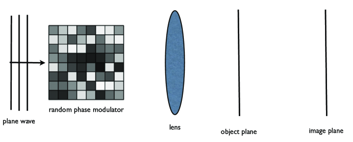
Figure 1. The imaging geometry for point objects

A main ingredient of the proposed approach is random illumination which has recently been used extensively for wavefront reconstruction and imaging [1, 19, 30]. Here we consider random phase modulation (RPM) which is a random perturbation of the phase of a wavefront while maintaining the amplitude of the near field beam almost constant. The advantage of phase modulation, compared to amplitude modulation, is the lossless energy transmission of an incident wavefront through the modulator. In optics RPM can be created by random phase plates, digital holograms or liquid crystal panels [8, 34].

3. Main results for point objects

We assume that as a result of $p$ independent realizations of random phase modulators the incident field at the grid points can be represented as $e^{\imath\theta_{kj}},k=1,...,p,j=1,...,N$ where $\theta_{kj}$ are i.i.d uniform random variables in $[0,2\pi]$ (i.e. circularly symmetric). The information about $\theta_{kj}$ is incorporated in the sensing matrix.

Let the scattered field $u^{\rm s}_{k}$ is measured and collected by $n$ sensors located at ${\mathbf{a}}_{l},l=1,...,n$. Let $X=(\tau_{j})_{1}^{N}\in\mathbb{C}^{N}$ be the object vector and $Y=(Y_{i})=(u_{k}^{\rm s}({\mathbf{a}}_{j}))\in\mathbb{C}^{np},i=(k-1)n+j,j=1,...,n,$ the data vector.

After proper normalization, the data vector $Y$ can be written as (2) with the sensing matrix ${\mathbf{\Phi}}$ being the column-normalized version of $[{G_{\rm par}}({\mathbf{a}}_{l},\mathbf{r}_{j})u^{\rm i}_{k}(\mathbf{r}_{j})]$, i.e.

(25) $$\phi_{ij} = {1\over\sqrt{np}}e^{\imath\omega|x_{j}-\xi_{l}|^{2}/(2z_{0})}e^{\imath\omega|y_{j}-\eta_{l}|^{2}/(2z_{0})}e^{\imath\theta_{kj}},\quad i=(k-1)n+l.$$

Here $m=np$ is the number of data.

Our first result is a performance guarantee for the OST with random illumination in the diffraction-limited case satisfying the Rayleigh resolution criterion.

Theorem 1.

Let

(26) $$N^{2}\leq{\delta\over 2}e^{K^{2}/2},\quad\delta,K>0.$$

Suppose

(27) $${np}\geq 40K^{4}\log{N}$$

and

(28) $${A\ell\over\lambda z_{0}}=1.$$

Then with probability at least

(29) $$1-2\delta-4t\sqrt{2\over\pi}-{4\over\sqrt{p}}-{4\over\sqrt{n}}-8Ne^{-12t^{2}\sqrt{N-1\over np}},\quad\forall t>0$$

OST with the threshold (6) can localize exactly $s$ objects satisfying (7)-(8).

Remark 1.

The constants $\delta$ and $K$ in (26) are controlling parameters. $\delta$ can be adjusted to control the lower bound (29) for success probability and then $K$ can be adjusted to control the number of grid points in the computation domain and the number of data.

For example, suppose $\delta=1\%$ is acceptable. Then (26) with $K=10$ implies a computation domain of about $0.1e^{25}/\sqrt{2}$ grid points.

Proof.

The proof of Theorem 1 relies on Proposition 2 and the following three lemmas.

Lemma 1.

Under (26), the worst case coherence satisfies

(30) $$\mathbb{P}\left\{\mu({\mathbf{\Phi}})\leq{aK\sqrt{2}\over\sqrt{p}}+{2K^{2}\over\sqrt{np}}\right\}\geq 1-2\delta$$

where $a$ is given by (35).

In particular, if (28) holds then $a=0$ and (30) becomes

(31) $$\mathbb{P}\left\{\mu({\mathbf{\Phi}})\leq{2}K^{2}/\sqrt{np}\right\}\geq 1-2\delta.$$

The proof of Lemma 1 is given in Section 5. The utility of estimate (30) lies in the situation where both the aperture and the sensor number are limited but the number of probe waves is exceedingly large (see Remark 3). For the proof of Theorem 1 we need the estimate (31).

Lemma 2.

Under the assumption (28),

(32) $$\mathbb{P}\left[\mu({\mathbf{\Phi}})\geq{2t_{1}t_{2}\over\sqrt{{np}}}\right]\geq\left(1-2t_{1}\sqrt{2\over\pi}-{4\over\sqrt{p}}\right)\left(1-2t_{2}\sqrt{2\over\pi}-{4\over\sqrt{n}}\right).$$

Lemma 2 is an easy consequence of the Berry-Esseen theorem and its proof is given in Section 5.2.

Lemma 3.

Let (28) hold true. Then for any $c>0$

(33) $$\mathbb{P}\left\{\nu({\mathbf{\Phi}})\leq{c\over{np}}\right\}\geq 1-8Ne^{-{c\over 2}\sqrt{{N-1\over np}}}.$$

The proof of Lemma 3 is given in Section 6.

First of all, by the upper bound (30) for the worst case coherence and setting $c_{1}=2K^{2}$ in (4) then the first inequality of (4) holds with probability at least $1-2\delta$. The second inequality of (4) follows from (26) and (27) and holds with probability at least $1-2\delta$.

Second, the lower bound (32) for the worst case coherence, with $t_{1}=t_{2}=t$, and the upper bound (33), with $c=24t^{2}$, for the average coherence imply that (5) holds with probability at least

$$1-4t\sqrt{2\over\pi}-{4\over\sqrt{p}}-{4\over\sqrt{n}}-8Ne^{-12t^{2}\sqrt{N-1\over np}}.$$

This completes the proof of Theorem 1. ∎

Our second result is a performance guarantee for the Lasso with random illumination.

Theorem 2.

Let (26) hold and suppose

(34) $${aK\sqrt{2}\over\sqrt{p}}+{2K^{2}\over\sqrt{np}}\leq{a_{0}\over\log{N}}$$

where

(35) $$a=\max_{j\neq j^{\prime}}\left|\mathbb{E}\left(e^{\imath\xi_{l}\omega(x_{j^{\prime}}-x_{j})/z_{0}}\right)\mathbb{E}\left(e^{\imath\eta_{l}\omega(y_{j^{\prime}}-y_{j})/z_{0}}\right)\right|.$$

Assume that the $s$ objects are real-valued and satisfy (12) and

(36) $$s\leq{c_{0}np\over 2\log{N}}.$$

Then the Lasso estimate $\hat{X}$ with $\gamma=2\sqrt{2\log{N}}$ has the same support as $X$ with probability at least

(37) $$1-2\delta-\rho n(n-1){\pi\over 2}\sqrt{np-1\over N}-2n^{2}p(p-1)e^{-{N\over(np-1)^{2}}}$$

$$\quad-2N^{-1}((2\pi\log N)^{-1/2}+sN^{-1})-\mathcal{O}(N^{-2\log 2})).$$

Remark 2.

While it requires that $N\gg np$ for the bound (29) to approach unity, it demands a much stronger assumption $N\gg\max\{pn^{5},p^{2}n^{2}\}$ for the bound (37) to behave the same way. Numerical evidences indicate the latter to be a pessimistic estimate.

For the special case of single sensor $n=1$, the probability lower bound (37) is substantially improved and requires $N\gg p^{2}$ to approach unity. On the other hand, for (29) to approach unity, it is necessary that $n\to\infty$ (hence $n=1$ is not an option).

Remark 3.

The superresolution effect can occur when the number $p$ of random probes is large. Consider, for example, the case of $n=1$ and hence the aperture $A$ is essentially zero. Since $a\leq 1$, the condition

$${K\sqrt{2}+2K^{2}\over\sqrt{p}}\leq{a_{0}\over\log{N}}$$

and

$$s\leq{c_{0}p\over 2\log{N}}$$

implies that the Lasso with $\gamma=2\sqrt{2\log{N}}$ recovers exactly the support of $s$ objects with probability at least that given by (37).

This superresolution effect should be compared to that with deterministic near-field illumination [20].

Proof.

The proof of Theorem 2 uses Proposition 3, Lemma 1 and the following operator-norm bound.

Lemma 4.

We have

(38) $$\mathbb{P}\left\{\|{\mathbf{\Phi}}\|^{2}_{2}<{2N\over np}\right\}\geq 1-\rho n(n-1){\pi\sqrt{np-1}\over 2\sqrt{N}}-2n^{2}p(p-1)e^{-{N\over(np-1)^{2}}}.$$

On one hand, Lemma 1 and (34) imply that (10) holds with probability at least $1-2\delta$.

On the other hand, Lemma 4 and (36) imply that (11) holds with probability at least given by the right hand side of (38).

Combining the two and using Proposition 3 we obtain the desired statement of Theorem 2.

∎

To further demonstrate the advantage of random illumination, let us consider the imaging set-up of multistatic responses (MR) which consists of an array of $n$ fixed transceivers which are both sources and sensors (i.e. transceivers). One by one, each transceiver of the array emits an impulse and the entire array of transceivers records the echo. Each transmitter-receiver pair gives rise to a datum and there are altogether $n^{2}$ data forming a data matrix called the multistatic response matrix. By the reciprocity of the wave equation, the MR matrix is symmetric and hence has at most $n(n+1)/2$ degrees of freedom.

Recalling the coherence and operator norm bounds established in [24] and using Proposition 3 as in the proof of Theorem 2 (below), we have the following result [24] analogous to Theorem 2.

Proposition 5.

Let the locations of the $n$ transceivers be i.i.d. uniform random variables in $[0,A]^{2}$. Let (27) and (28) hold true.

Suppose

$$n\geq{K^{2}\log{N}\over a_{0}}$$

and that the $s$ real-valued objects satisfy (12) and

(39) $$s\leq{c_{0}n(n+1)\over 4\log{N}}.$$

Then the Lasso estimate $\hat{X}$ with $\gamma=2\sqrt{2\log{N}}$ has the same support as $X$ with probability at least

(40) $$1-2\sqrt{2\delta}-{\rho n^{5/2}(n+1)^{5/2}\over\pi 2^{5/2}N^{1/2}}-2N^{-1}((2\pi\log N)^{-1/2}+sN^{-1})-\mathcal{O}(N^{-2\log 2})).$$

Remark 4.

The main drawback of the lower bound (40) lies in the third term which requires $N\gg n^{10}$ to diminish.

More generally, one can consider the case of $p$ transmitters and $n$ receivers, all randomly and independently distributed in $[0,A]^{2}$. Then an extension of the bound (40), which is omitted here, requires $N\gg n^{5}p^{5}$ (cf. [21]).

From dimension count, a fair comparison with Theorem 2 would be to set $p=(n+1)/2$ and match their degrees of freedom, i.e. $n(n+1)/2$. However, Proposition 5 does not guarantee superresolution when (28) is violated preventing the worst case coherence from being sufficiently small due to the deterministic nature of the illumination. Also, the probability lower bound (40) has a less favorable scaling behavior ($N\gg n^{10}$) than (37) for $p=(n+1)/2$ ($N\gg n^{6}$, cf. Remark 2). Indeed, the numerical simulations show the recovery with random illumination has a higher success rate than the MR recovery (Figures 3 and 4).

4. Sparse extended objects

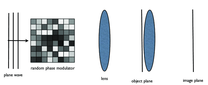
Figure 2. The imaging geometry for extended objects

We extend the above results to the case of sparse extended objects here (Figure 2).

We pixelate the sparse extended object with $N$ pixels $\square_{j},j=1,...,N$ of size $\ell$ to create a piecewise constant approximation of the object. The centers of the pixels are identified as ${\mathcal{L}}$ given in (18). Let $O(\mathbf{r})$ be a the original object and $O_{\ell}$ its $\ell$-discretization, i.e.

$$O_{\ell}=\sum_{j=1}^{N}\mathbb{I}_{\square_{j}}O(\mathbf{r}_{j})$$

where $\mathbb{I}_{\square_{j}}$ is the indicator function of the pixel $\square_{j}$. We reconstruct the discrete approximation $O_{\ell}$ by determining the object function restricted to ${\mathcal{L}}$, denoted still by $X=(O(\mathbf{r}_{j}))$, by compressed sensing techniques.

Under the random illumination $u^{\rm i}_{k}$, pixel $\square_{j}$ now produces a signal at the sensor ${\mathbf{a}}_{l}$ of the form

$$O(\mathbf{r}_{j})\int_{\square_{j}}{G_{\rm par}}(\mathbf{r},{\mathbf{a}}_{l})e^{-\imath\omega x^{2}/(2z_{0})}e^{-\imath\omega y^{2}/(2z_{0})}u^{\rm i}_{k}(x,y)dxdy$$

where the quadratic phase factors are due to the presence of a parabolic lens immediately after the object plane (Figure 2). This lens is introduced here to simplify our analysis. In practice, the lens is not needed and should have a negligible effect on performance.

As for the case of point objects we assume that as a result of the RPM $u^{\rm i}_{k}$ takes a constant value $e^{\imath\theta_{kj}}$ in pixel $\square_{j}$ and that $\theta_{kj}$ are i.i.d. random variables in $[0,2\pi]$ as a result of random phase modulation.

The total signal produced by $O_{\ell}$ and detected at sensor ${\mathbf{a}}_{l}$ is

$$\sum_{j}O(\mathbf{r}_{j})e^{\imath\theta_{kj}}\int_{\square_{j}}{G_{\rm par}}(\mathbf{r},{\mathbf{a}}_{l})e^{-\imath\omega x^{2}/(2z_{0})}e^{-\imath\omega y^{2}/(2z_{0})}dxdy$$

$$= \sum_{j}O(\mathbf{r}_{j})e^{\imath\theta_{kj}}e^{\imath\omega\xi_{l}^{2}/(2z_{0})}e^{\imath\omega\eta_{l}^{2}/(2z_{0})}e^{-\imath\omega\xi_{l}x_{j}/z_{0}}e^{-\imath\omega\eta_{l}y_{j}/z_{0}}\int_{\square}e^{-\imath\omega\xi_{l}x/z_{0}}e^{-\imath\omega\eta_{l}y/z_{0}}dxdy,$$

plus an error term $E_{kl}$ which includes the discretization error and external noise where $\square$ denotes the square of size $\ell$ centered at the origin. Since

(41) $$\int_{\square}e^{-\imath\omega\xi_{l}x/z_{0}}e^{-\imath\omega\eta_{l}y/z_{0}}dxdy={2z_{0}\over\omega\xi_{l}\ell}\sin{\left(\omega\xi_{l}\ell\over 2z_{0}\right)}{2z_{0}\over\omega\eta_{l}\ell}\sin{\left(\omega\eta_{l}\ell\over 2z_{0}\right)}\equiv g({\mathbf{a}}_{l})$$

independent of the pixel index, we can normalize the data by dividing the signal at sensor $l$ by this number as long as

(42) $${\xi_{l}\ell\over\lambda z_{0}},\,\,{\eta_{l}\ell\over\lambda z_{0}}<1,\quad\forall l=1,\ldots,n.$$

Dividing the data further by the phase factors $e^{\imath\omega\xi_{l}^{2}/(2z_{0})}e^{\imath\omega\eta_{l}^{2}/(2z_{0})}$ and $\sqrt{np}$, we write the signal model as (2) with the sensing matrix element

(43) $$\phi_{ij} = {1\over\sqrt{np}}e^{\imath\theta_{kj}}e^{-\imath\omega\xi_{l}x_{j}/z_{0}}e^{-\imath\omega\eta_{l}y_{j}/z_{0}},\quad i=(k-1)n+l.$$

The difference between the signals produced by $O$ and its discretization $O_{\ell}$ is the discretization error $E_{\rm disc}$. How small must $\ell$ be in order for the $\ell_{2}$-norm of the discretization error $E_{\rm disc}$ be less than, say, $\varepsilon$ after rewriting the signal model as (2)? This can be estimated as follows.

First, by the inequality $\|E_{\rm disc}\|_{2}\leq\|E_{\rm disc}\|_{\infty}\sqrt{np}$ it suffices to show $\|E_{\rm disc}\|_{\infty}\leq\varepsilon/\sqrt{np}$.

Since

$$u^{\rm i}_{k}(\mathbf{r})=\sum_{j=1}^{N}e^{\imath\theta_{kj}}\mathbb{I}_{\square_{j}}(\mathbf{r})$$

is the illumination field, the uncontaminated signal detected by sensor ${\mathbf{a}}_{l}$ in the absence of external noise in the signal model (2) is

(44) $$({\mathcal{F}}O)_{i}={1\over g({\mathbf{a}}_{l})}\sum_{j=1}^{N}e^{\imath\theta_{kj}}\int_{\square_{j}}O(x,y)e^{-\imath\omega\xi_{l}x_{j}/z_{0}}e^{-\imath\omega\eta_{l}y_{j}/z_{0}}dxdy,$$

for $i=(k-1)n+l.$ On the other hand we have

$$({\mathcal{F}}O_{\ell})_{i}={1\over g({\mathbf{a}}_{l})}\sum_{j=1}^{N}e^{\imath\theta_{kj}}O(\xi_{j},y_{j})\int_{\square_{j}}e^{-\imath\omega\xi_{l}x_{j}/z_{0}}e^{-\imath\omega\eta_{l}y_{j}/z_{0}}dxdy$$

for $i=(k-1)n+l.$ By definition

$$E_{\rm disc}={\mathcal{F}}O-{\mathcal{F}}O_{\ell}\in\mathbb{C}^{pn}$$

and hence

(45) $$\|E_{\rm disc}\|_{\infty} \leq {\|O-O_{\ell}\|_{L^{1}}\over\min_{l}|g({\mathbf{a}}_{l})|}$$

where $\|\cdot\|_{L^{1}}$ denotes

$$\|f\|_{L^{1}}=\int|f(x,y)|dxdy,$$

i.e. the norm of the function space $L^{1}$. Therefore we have the following statement.

Lemma 5.

If

(46) $${\|O-O_{\ell}\|_{L^{1}}}\leq{\varepsilon\over\sqrt{np}}\min_{l}|g({\mathbf{a}}_{l})|$$

then

$$\|E_{\rm disc}\|_{2}\leq\varepsilon.$$

Remark 5.

The presence of the factor $(np)^{-1/2}$ in (46) is due to the transition from $L^{1}$ function space norm to the discrete $\ell_{2}$-norm.

Since the sensing matrix (25) for the point objects can be written as

$$\mathbf{D}_{1}{\mathbf{\Phi}}\mathbf{D}_{2}$$

where ${\mathbf{\Phi}}$ is as (43) and

$$\mathbf{D}_{1} = \hbox{diag}(e^{\imath\omega\xi_{l}^{2}/(2z_{0})}e^{\imath\omega\eta_{l}^{2}/(2z_{0})})$$

$$\mathbf{D}_{2} = \hbox{diag}(e^{\imath\omega x_{j}^{2}/(2z_{0})}e^{\imath\omega y_{j}^{2}/(2z_{0})})$$

are diagonal, unitary matrices. All the preceding results, including Theorems 1 and 2, can be proved for the sensing matrix (43) by minor modification of the previous arguments.

However, the object vector $X=(O(\mathbf{r}_{j}))$ of an extended object generally does not fall into the category of random point objects assumed in either Proposition 2 or 3 since by definition the discrete approximation of an extended object must cluster in aggregates and its amplitude typically changes continuously. So we take an alternative approach below by resorting to the minimization principle (15) of BPDN.

The RIC for a structured sensing matrix such as (43) is difficult to estimate directly except for the case of single shot ($p=1$) and the case of one sensor ($n=1$). For the one-sensor case, (43) with $(\xi_{l},\eta_{l})=(0,0)$ is the complex-value version of the random i.i.d. Bernoulii matrix:

(47) $$\phi_{kj}={1\over\sqrt{p}}e^{\imath\theta_{kj}},$$

whose RIC can be easily estimated by the same argument given in [4]. The single sensor imaging set-up resembles that of Rice’s single-pixel camera [19] which employs a discrete random screen instead of a random phase modulator.

For the single-shot case, the sensing matrix (43) is equivalent to the random partial Fourier matrix, modulo an unitary diagonal matrix, and the standard RIP estimate [29] requires the Rayleigh criterion (28) to be met which guarantees (42) with probability one. However, there exists a small probability of ${\mathbf{a}}_{l}=(\xi_{l},\eta_{l})$ falling near the boundary of the aperture and hence a small value of $|g({\mathbf{a}}_{l})|$. Normalizing the data by $|g({\mathbf{a}}_{l})|$ then carries a small risk of magnifying the errors.

For the general set-up with multiple shots and sensors, we use the mutual coherence to bound the RIC trivially as follows.

Proposition 6.

For any $s\in\mathbb{N}$ we have

$$\delta_{s}\leq\mu({\mathbf{\Phi}})(s-1).$$

Combining Lemma 1, Propositions 4 and 6 we obtain the following result.

Theorem 3.

Under (26), the RIC bound (17) holds true with probability at least $1-2\delta$ for the sensing matrix (43) and sparsity up to

(48) $$s<{1\over 2}+\left({1\over\sqrt{2}}-{1\over 2}\right)\left({aK\sqrt{2}\over\sqrt{p}}+{2K^{2}\over\sqrt{np}}\right)^{-1}$$

where

$$a=\max_{j\neq j^{\prime}}\left|\mathbb{E}\left(e^{\imath\xi_{l}\omega(x_{j^{\prime}}-x_{j})/z_{0}}\right)\mathbb{E}\left(e^{\imath\eta_{l}\omega(y_{j^{\prime}}-y_{j})/z_{0}}\right)\right|$$

c.f. (35).

Furthermore, suppose the total error in the data is $E=E_{\rm disc}+E_{\rm ext}$ where $E_{\rm disc}$ and $E_{\rm ext}$ are, respectively, the discretization error and the external noise. Then the reconstruction $\hat{X}$ by BPDN satisfies the error bound

(49) $$\|\hat{X}-X\|_{2}\leq C_{1}s^{-1/2}\|X-X^{(s)}\|_{1}+C_{2}\left(\|E_{\rm disc}\|_{2}+\|E_{\rm ext}\|_{2}\right)$$

for all $s$ satisfying (48).

Remark 6.

Since BPDN does not guarantee exact localization, an appropriate metric for resolution can be formulated in terms of the smallest pixel size $\ell_{\rm min}$ and largest sparsity $s$ such that (49) holds true with both the discretization error $E_{\rm disc}$ and $s^{-1/2}\|X-X^{(s)}\|_{1}$ being reasonably small.

The right definition of “small errors”, however, is problem specific. The discrete norms ($\ell_{1}$- or $\ell_{2}$- norm) tend to go up simply because the effective sparsity increases. Hence the right metric of reconstruction error should be properly normalized by the size of the object. For example, consider the special case when $X$ is $s$-sparse. Then we can rewrite (49) as

(50) $$s^{-1/2}\|\hat{X}-X\|_{2}\leq C_{2}\|E_{\rm ext}\|_{2}s^{-1/2}+C_{2}\|E_{\rm disc}\|_{2}s^{-1/2}$$

whose left hand side is a measure of the reconstruction error per pixel of size $\ell$.

Below the diffraction limit $A\ell/(\lambda z_{0})<1$ ($a\neq 0$), one can reduce the discretization error by reducing the pixel size according to Lemma 5. On the other hand, the sparsity $s$ increases in proportion to $\ell^{-2}$ for a two-dimensional extended object. To satisfy (48) the smallest admissible pixel size $\ell_{\rm min}$ is bounded from below roughly by

(51) $$\ell_{\rm min}\stackrel{{\scriptstyle>}}{{\sim}}{a^{1/2}p^{-1/4}}$$

meaning that the minimum super-resolved scale decreases at least as fast as the negative quarter power of the number of random illuminations.

For the diffraction-limited case $a=0$, we have instead

$$\ell_{\rm min}\stackrel{{\scriptstyle>}}{{\sim}}{n^{-1/4}p^{-1/4}}$$

which is more favorable than (51) for $n\gg 1$. However, the discretization error bound (Lemma 5) is less useful in this case.

5. Worst-case coherence bound

5.1. Proof of Lemma 1: upper bound

Proof.

Summing over ${\mathbf{a}}_{l},l=1,...,n$ we obtain

(52) $$\sum_{k=1}^{p}\sum_{l=1}^{n}\phi^{*}_{i{j^{\prime}}}\phi_{ij} = e^{\imath\omega(x_{j}^{2}+y_{j}^{2}-x_{j^{\prime}}^{2}-y_{j^{\prime}}^{2})/(2z_{0})}{1\over np}\sum_{k=1}^{p}e^{\imath(\theta_{kj}-\theta_{kj^{\prime}})}\sum_{l=1}^{n}e^{\imath\xi_{l}\omega(x_{j^{\prime}}-x_{j})/z_{0}}e^{\imath\eta_{l}\omega(y_{j^{\prime}}-y_{j})/z_{0}}.$$

We shall estimate the two summations separately.

First consider the summation over random illuminations $k=1,...,p$. Define the random variables $A_{l},B_{l},l=1,...,n$, as

(53) $$A_{l} = \cos{\left[\theta_{kj}-\theta_{kj^{\prime}}\right]}$$

(54) $$B_{l} = \sin{\left[\theta_{kj}-\theta_{kj^{\prime}}\right]}$$

and let

(55) $$S_{p}=\sum_{l=1}^{p}(A_{l}+iB_{l}).$$

To estimate $S_{p}$, we recall the Hoeffding inequality [27].

Proposition 7.

Let $A_{1}+iB_{1},...,A_{p}+iB_{p}$ be independent random variables. Assume that $A_{l},B_{l}\in[a_{l},b_{l}],l=1,...,p$ almost surely. Then we have

(56) $$\mathbb{P}\left[\left|S_{p}-\mathbb{E}S_{p}\right|\geq pt\right]\leq 4\exp{\left[-{p^{2}t^{2}\over\sum_{l=1}^{p}(b_{l}-a_{l})^{2}}\right]}$$

for all positive values of $t$.

We apply the Hoeffding inequality to $S_{p}$ with $a_{l}=-1,b_{l}=1,l=1,...,p$ and

$$t=K\sqrt{2\over p},\quad K>0$$

to obtain

(57) $$\mathbb{P}\left[p^{-1}\left|\sum_{k=1}^{p}e^{\imath(\theta_{kj}-\theta_{kj^{\prime}})}\right|\geq{K\sqrt{2\over p}}\right]\leq 4e^{-K^{2}/2}.$$

Note the dependence of $S_{p}$ on $\theta_{kj}-\theta_{kj^{\prime}}$ and the symmetry: $|S_{p}(\theta_{kj^{\prime}}-\theta_{kj})|=|S_{p}(\theta_{kj^{\prime}}-\theta_{kj})|$. As a consequence, there may be $N(N-1)/2$ different values of $S_{p}$. By union bound with (57), we obtain

(58) $$\mathbb{P}\left[p^{-1}\max_{j\neq j^{\prime}}\left|\sum_{k=1}^{p}e^{\imath(\theta_{kj}-\theta_{kj^{\prime}})}\right|\geq{K\sqrt{2\over p}}\right]\leq 2N(N-1)e^{-K^{2}/2}\leq\delta$$

by (26).

Next consider the summation, denoted by $T_{n}$, over the sensor locations $l=1,...,n$ in (52):

$$T_{n}=\sum_{l=1}^{n}e^{\imath\xi_{l}\omega(x_{j^{\prime}}-x_{j})/z_{0}}e^{\imath\eta_{l}\omega(y_{j^{\prime}}-y_{j})/z_{0}}.$$

By the same argument we obtain

$$\mathbb{P}\left[\max_{j^{\prime}\neq j}n^{-1}\left|T_{n}-\mathbb{E}T_{n}\right|\geq K\sqrt{2\over n}\right] \leq 2N(N-1)e^{-{K^{2}/2}}$$

and hence

(59) $$\mathbb{P}\left[\max_{j^{\prime}\neq j}{1\over n}\left|T_{n}\right|\geq a+K\sqrt{2\over n}\right] \leq \delta,\quad a=\max_{j\neq j^{\prime}}{1\over n}|\mathbb{E}T_{n}|$$

by (26).

By the mutual independence of $\xi_{l}$ and $\eta_{l}$ we have

$$a=\max_{j\neq j^{\prime}}{1\over n}\left|\mathbb{E}T_{n}\right| = \max_{j\neq j^{\prime}}{1\over n}\left|\sum_{l=1}^{n}\mathbb{E}\left(e^{\imath\xi_{l}\omega(x_{j^{\prime}}-x_{j})/z_{0}}\right)\mathbb{E}\left(e^{\imath\eta_{l}\omega(y_{j^{\prime}}-y_{j})/z_{0}}\right)\right|$$

$$= \max_{j\neq j^{\prime}}\left|\mathbb{E}\left(e^{\imath\xi_{l}\omega(x_{j^{\prime}}-x_{j})/z_{0}}\right)\mathbb{E}\left(e^{\imath\eta_{l}\omega(y_{j^{\prime}}-y_{j})/z_{0}}\right)\right|$$

since $\xi_{l},\eta_{l},l=1,...,n$ are independently identically distributed.

Combining (59) and (58) and noting the independence of these two events, we obtain

$$\mu({\mathbf{\Phi}})\leq{aK\sqrt{2}\over\sqrt{p}}+{2K^{2}\over\sqrt{np}}$$

with probability at least $1-2\delta$.

Simple calculation with the uniform distribution on the set ${\mathcal{D}}$ given in (22) yields

(60) $$\left|\mathbb{E}\left(e^{\imath\xi_{l}\omega(x_{j^{\prime}}-x_{j})/z_{0}}\right)\mathbb{E}\left(e^{\imath\eta_{l}\omega(y_{j^{\prime}}-y_{j})/z_{0}}\right)\right| = 0,\quad j^{\prime}\neq j$$

if (28) holds. In this case,

$$\mu({\mathbf{\Phi}})\leq{2}K^{2}/\sqrt{np}$$

with probability $1-2\delta$.

∎

5.2. Proof of Lemma 2: Lower bound

Proof.

The Berry-Esseen theorem [25] states that the distribution of the sum of $m$ independent and identically distributed zero-mean random variables normalized by its standard deviation, differs from the unit Gaussian distribution by at most $C\rho/(\sigma^{2}\sqrt{m})$, where $\sigma^{2}$ and $\rho$ are respectively the variance and the absolute third moment of the parent distribution, and $C$ is a distribution-independent absolute constant which is not greater than 0.7655 [32].

We shall apply the Berry-Esseen theorem to the two summations, denoted by $S_{p}$ and $T_{n}$ respectively, on the right hand side of (52).

The complex-valued random variables involved can be treated as $\mathbb{R}^{2}$-valued random variables. Under (28) the variance of these random variables is $1/2$ and the absolute third moment is $4/(3\pi)$.

Let $F_{1},F_{2}$ be the cumulative distributions of the real and imaginary parts of $p^{-1/2}S_{p}$ and $G_{1},G_{2}$ the cumulative distributions of the real and imaginary parts of $n^{-1/2}T_{n}$. Let $\Psi$ be the cumulative distribution of the standard normal random variable. We have by the Berry-Esseen theorem

(61) $$\sup_{t}|F_{i}(t)-\Psi(t)| \leq {C8\sqrt{2}\over 3\pi\sqrt{p}},\quad i=1,2$$

(62) $$\sup_{t}|G_{i}(t)-\Psi(t)| \leq {C8\sqrt{2}\over 3\pi\sqrt{n}},\quad i=1,2.$$

Since $C\leq 0.7655$, we can replace the right hand side of (61) and (62)) by $p^{-1/2}$ and $n^{-1/2}$ respectively for the sake of notational simplicity. Hence

$$|F_{i}(t)-F_{i}(-t)| \leq |\Psi(t)-\Psi(-t)|+{2\over\sqrt{p}}$$

$$|G_{i}(t)-G_{i}(-t)| \leq |\Psi(t)-\Psi(-t)|+{2\over\sqrt{n}}$$

$\forall t$. For small $t>0$ we can bound the above expressions by

$$|F_{i}(t)-F_{i}(-t)| \leq t\sqrt{2\over\pi}+{2\over\sqrt{p}}$$

$$|G_{i}(t)-G_{i}(-t)| \leq t\sqrt{2\over\pi}+{2\over\sqrt{n}}$$

which imply

$$\mathbb{P}\left[p^{-1/2}|S_{p}|\leq t\sqrt{2}\right] \leq 2t\sqrt{2\over\pi}+{4\over\sqrt{p}}$$

$$\mathbb{P}\left[n^{-1/2}|T_{n}|\leq t\sqrt{2}\right] \leq 2t\sqrt{2\over\pi}+{4\over\sqrt{n}}$$

and consequently

(63) $$\mathbb{P}\left[{|S_{p}T_{n}|\over np}\geq{2t_{1}t_{2}\over\sqrt{{np}}}\right]\geq\left(1-2t_{1}\sqrt{2\over\pi}-{4\over\sqrt{p}}\right)\left(1-2t_{2}\sqrt{2\over\pi}-{4\over\sqrt{n}}\right)$$

which is what we want to prove.

∎

6. Average coherence bound: proof of Lemma 3

Proof.

Write

$$\nu({\mathbf{\Phi}}) = {1\over N-1}\max_{j^{\prime}}\left|\sum_{l=1}^{n}\sum_{k=1}^{p}\sum_{j\neq j^{\prime}}\phi^{*}_{ij^{\prime}}\phi_{ij}\right|,\quad i=(k-1)n+l$$

and consider the sums over $k$ and $j$ simultaneously with a fixed $j^{\prime}$ and fixed $n$ sensor locations. This is a summation of $p\cdot N$ independent random variables $\phi_{ij^{\prime}}\phi_{ij}$ each bounded by $n^{-1}p^{-1}$ in absolute value. Note that

(64) $$\mathbb{E}_{\xi,\eta}\left[\phi^{*}_{ij^{\prime}}\phi_{ij}\right]=0,\quad\forall j,j^{\prime},i$$

since $\theta_{kj}$ are uniformly distributed in $[0,2\pi]$. Applying Hoeffding inequality with

$$t={c_{1}\over(N-1)^{1/2}p^{3/2}n},\quad c>0$$

we have

(65) $$\mathbb{P}_{\xi,\eta}\left[{1\over N-1}\left|\sum_{k=1}^{p}\sum_{j\neq j^{\prime}}\phi_{ij^{\prime}}\phi_{ij}\right|\geq{c_{1}\over(N-1)^{1/2}p^{1/2}n}\right]\leq 4e^{-c_{1}^{2}}$$

where $\mathbb{P}_{\xi,\eta}$ is the probability conditioned on fixed $\xi=(\xi_{j}),\eta=(\eta_{j})\in\mathbb{R}^{n}$. In analyzing the sum over $l=1,...,n$ we shall restrict to the event

$${\mathcal{A}}=\left\{\Theta=[\theta_{kj}]:{1\over N-1}\left|\sum_{k=1}^{p}\sum_{j\neq j^{\prime}}\phi_{ij^{\prime}}\phi_{ij}\right|<{c_{1}\over np^{1/2}(N-1)^{1/2}}\,\,\hbox{for almost all sensor locations}.\right\}$$

Since there are at most $N$ possible sensor locations, by (65)

(66) $$\mathbb{P}({\mathcal{A}}^{c})\leq 4Ne^{-c_{1}^{2}}$$

where ${\mathcal{A}}^{c}$ denotes the complement of ${\mathcal{A}}$.

Let

$$Z_{j^{\prime}l}={1\over N-1}\sum_{k=1}^{p}\sum_{j\neq j^{\prime}}\phi^{*}_{ij^{\prime}}\phi_{ij}$$

and $\mathbb{E}_{\mathcal{A}}$ is the expectation conditioned on the event ${\mathcal{A}}$.

We proceed with the following estimate

(67) $$\mathbb{P}\left[\max_{j^{\prime}}\left|\sum_{l=1}^{n}\left(Z_{j^{\prime}l}-\mathbb{E}_{\mathcal{A}}Z_{j^{\prime}l}\right)\right|\geq{c_{2}\over\sqrt{np(N-1)}}\right]$$

$$= \mathbb{P}_{\mathcal{A}}\left[\max_{j^{\prime}}\left|\sum_{l=1}^{n}\left(Z_{j^{\prime}l}-\mathbb{E}_{\mathcal{A}}Z_{j^{\prime}l}\right)\right|\geq{c_{2}\over\sqrt{np(N-1)}}\right]\mathbb{P}({\mathcal{A}})$$

$$+\mathbb{P}_{{\mathcal{A}}^{c}}\left[\max_{j^{\prime}}\left|\sum_{l=1}^{n}\left(Z_{j^{\prime}l}-\mathbb{E}_{\mathcal{A}}Z_{j^{\prime}l}\right)\right|\geq{c_{2}\over\sqrt{np(N-1)}}\right]\mathbb{P}({\mathcal{A}}^{c})$$

$$\leq \mathbb{P}_{\mathcal{A}}\left[\max_{j^{\prime}}\left|\sum_{l=1}^{n}\left(Z_{j^{\prime}l}-\mathbb{E}_{\mathcal{A}}Z_{j^{\prime}l}\right)\right|\geq{c_{2}\over\sqrt{np(N-1)}}\right]+4Ne^{-c_{1}^{2}},\quad c_{1},c_{2}>0$$

by (66) where $\mathbb{P}_{\mathcal{A}}$ and $\mathbb{P}_{{\mathcal{A}}^{c}}$ are respectively the probabilities conditioned on the events ${\mathcal{A}}$ and ${\mathcal{A}}^{c}$.

Applying Hoeffding’s inequality with

$$t={c_{2}\over p^{1/2}(N-1)^{1/2}n^{3/2}}$$

to estimate the first term on the right hand side of (67), we obtain

$$\mathbb{P}_{\mathcal{A}}\left[\left|\sum_{l=1}^{n}\left(Z_{j^{\prime}l}-\mathbb{E}_{\mathcal{A}}Z_{j^{\prime}l}\right)\right|\geq{c_{2}\over\sqrt{np(N-1)}}\right]\leq 4e^{-c_{2}^{2}/(2c_{1})^{2}}.$$

Maximizing over $j^{\prime}=1,...,m$ and using the union bound we then arrive at

(68) $$\mathbb{P}_{\mathcal{A}}\left[\max_{j^{\prime}}\left|\sum_{l=1}^{n}\left(Z_{j^{\prime}l}-\mathbb{E}_{\mathcal{A}}Z_{j^{\prime}l}\right)\right|\geq{c_{2}\over\sqrt{np(N-1)}}\right]\leq 4Ne^{-c_{2}^{2}/(2c_{1})^{2}}.$$

Using (67) and (68) with

$$c_{2}=c\sqrt{N-1\over np},\quad c_{2}=2{c_{1}^{2}},\quad c>0$$

we have

$${\mathbb{P}\left[\max_{j^{\prime}}\left|\sum_{l=1}^{n}\left(Z_{j^{\prime}l}-\mathbb{E}_{\mathcal{A}}Z_{j^{\prime}l}\right)\right|\geq{c\over{np}}\right]} \leq 8Ne^{-{c\over 2}\sqrt{{N-1\over np}}},\quad c>0,$$

which is what we set out to prove.

Note that

$$\mathbb{E}_{\Theta}Z_{j^{\prime}l}={1\over n}\mathbb{E}\left(e^{\imath\xi_{l}\omega(x_{j^{\prime}}-x_{j})/z_{0}}\right)\mathbb{E}\left(e^{\imath\eta_{l}\omega(y_{j^{\prime}}-y_{j})/z_{0}}\right),\quad\forall j^{\prime}=1,...,m,\quad l=1,...,n,\quad j^{\prime}\neq j$$

where $\mathbb{E}_{\Theta}$ is the expectation conditioned on $\Theta=(\theta_{kj})\in\mathbb{C}^{p\times n}$. If

$${1\over\rho}={A\ell\over\lambda z_{0}}\in\mathbb{N}$$

then

$$\mathbb{E}_{\Theta}Z_{j^{\prime}l}=0,\quad\forall j^{\prime}=1,...,m,\quad l=1,...,n$$

and hence

$$\mathbb{E}_{\mathcal{A}}Z_{j^{\prime}l}=0,\quad\forall j^{\prime}=1,...,m,\quad l=1,...,n.$$

∎

7. Operator norm bound: proof of Lemma 4

Proof.

It suffices to show that the matrix ${\mathbf{\Phi}}$ satisfies

(69) $$\|{np\over N}{\mathbf{\Phi}}{\mathbf{\Phi}}^{*}-\mathbf{I}_{np}\|_{2}<1$$

where $\mathbf{I}_{np}$ is the $np\times np$ identity matrix with the corresponding probability bound. Since the diagonal elements of ${np\over N}{\mathbf{\Phi}}{\mathbf{\Phi}}^{*}$ are unity, (69) would in turn follow from

(70) $$\mu\left({\mathbf{\Phi}}^{*}\right)<{1\over np-1}$$

by the Gershgorin circle theorem.

The pairwise coherence has the form

$${np\over N}\sum_{j=1}^{N}\phi_{ij}\phi^{*}_{i^{\prime}j} = {1\over N}e^{\imath\omega(\xi_{l}^{2}+\eta_{l}^{2}+\xi_{i}^{2}-\xi_{l^{\prime}}^{2}-\eta_{l^{\prime}}^{2})/(2z_{0})}\sum_{j=1}^{N}e^{\imath\omega x_{j}(\xi_{l^{\prime}}-\xi_{l})/z_{0}}e^{\imath\omega y_{j}(\eta_{l^{\prime}}-\eta_{l})/z_{0}}e^{\imath(\theta_{kj}-\theta_{k^{\prime}j})}.$$

There are two cases: (i) $k\neq k^{\prime}$, (ii) $k=k^{\prime},l\neq l^{\prime}$.

For case (i), $\theta_{kj}-\theta_{k^{\prime}j}$ are independent random variables for $j=1,...,N$. Applying Hoeffding inequality to

$$Z_{N}\equiv\sum_{j=1}^{N}e^{\imath\omega x_{j}(\xi_{l^{\prime}}-\xi_{l})/z_{0}}e^{\imath\omega y_{j}(\eta_{l^{\prime}}-\eta_{l})/z_{0}}e^{\imath(\theta_{kj}-\theta_{k^{\prime}j})}$$

we obtain

(71) $$\mathbb{P}\left[{1\over N}\left|Z_{N}\right|\geq t\right]\leq 4e^{-Nt^{2}}.$$

Set $t=\alpha/\sqrt{N}$, we have

$$\mathbb{P}\left[\left|{np\over N}\sum_{j=1}^{N}\phi_{ij}\phi^{*}_{i^{\prime}j}\right|\geq{\alpha\over\sqrt{N}}\right]\leq 4e^{-\alpha^{2}}$$

and thus

(72) $$\mathbb{P}\left[\sup_{k\neq k^{\prime}\atop\forall l,l^{\prime}}\left|{np\over N}\sum_{j=1}^{N}\phi_{ij}\phi^{*}_{i^{\prime}j}\right|\geq{\alpha\over\sqrt{N}}\right]\leq 2n^{2}p(p-1)e^{-\alpha^{2}}$$

by the union bound.

For case (ii), $\theta_{kj}-\theta_{k^{\prime}j}=0$ and $Z_{N}$ becomes a geometric series

$$Z_{N} = {e^{\imath\omega(\xi_{l^{\prime}}-\xi_{l})(x_{1}+\sqrt{N}\ell)/z_{0}}-e^{\imath\omega(\xi_{l^{\prime}}-\xi_{l})x_{1}/z_{0}}\over 1-e^{\imath\omega(\xi_{l^{\prime}}-\xi_{l})\ell/z_{0}}}\times{e^{\imath\omega(\eta_{l^{\prime}}-\eta_{l})(y_{1}+\sqrt{N}\ell)/z_{0}}-e^{\imath\omega(\eta_{l^{\prime}}-\eta_{l})y_{1}/z_{0}}\over 1-e^{\imath\omega(\eta_{l^{\prime}}-\eta_{l})\ell/z_{0}}}.$$

Thus,

$${np\over N}\left|\sum_{j=1}^{N}\phi_{ij}\phi^{*}_{i^{\prime}j}\right| \leq {1\over N}\left|{\sin{\omega\ell\sqrt{N}(\xi_{l^{\prime}}-\xi_{l})\over 2z_{0}}\over\sin{\omega\ell(\xi_{l^{\prime}}-\xi_{l})\over 2z_{0}}}\right|\cdot\left|{\sin{\omega\ell\sqrt{N}(\eta_{l^{\prime}}-\eta_{l})\over 2z_{0}}\over\sin{\omega\ell(\eta_{l^{\prime}}-\eta_{l})\over 2z_{0}}}\right|.$$

Let

$$\kappa=\min_{l\neq l^{\prime}}\min_{j\in\mathbb{Z}}\left\{\left|{\ell(\xi_{l^{\prime}}-\xi_{l})\over\lambda z_{0}}-j\right|,\left|{\ell(\eta_{l^{\prime}}-\eta_{l})\over\lambda z_{0}}-j\right|\right\}.$$

Clearly $\kappa$ is nonzero with probability one. For $l\neq l^{\prime}$ the probability density functions (PDF) for the random variables

$${\ell(\xi_{l^{\prime}}-\xi_{l})\over\lambda z_{0}},\quad{\ell(\eta_{l^{\prime}}-\eta_{l})\over\lambda z_{0}}$$

are either the symmetric triangular distribution or its self-convolution supported on $[-2\rho^{-1},2\rho^{-1}]$. In either case, their PDFs are bounded by $\rho$. Hence the probability that $\{\kappa>\beta\}$ for small $\beta>0$ is larger than

$$(1-2\rho\beta)^{n(n-1)/2}>1-\beta\rho n(n-1)$$

where the exponent counts the number of distinct unordered pairs $(l,l^{\prime})$. Note that the above analysis is independent of $k=k^{\prime}$. Since $\sin\theta\geq\theta,\forall\theta\in[0,\pi/2]$ we have that

(73) $$\mathbb{P}\left[\sup_{k=k^{\prime}\atop l\neq l^{\prime}}{np\over N}\left|\sum_{j=1}^{N}\phi_{ij}\phi^{*}_{i^{\prime}j}\right|\geq{\pi^{2}\over 4N\beta^{2}}\right]\leq\beta\rho n(n-1).$$

Setting

(74) $$\max\left\{{\alpha\over\sqrt{N}}\right\}<{\pi^{2}\over 4N\beta^{2}}={1\over np-1}$$

and using (72) and (73) we have

(75) $$\mathbb{P}\left[\sup_{i\neq i^{\prime}}{np\over N}\left|\sum_{j=1}^{N}\phi_{ij}\phi^{*}_{i^{\prime}j}\right|\geq{1\over np-1}\right]\leq\beta\rho n(n-1)+2n^{2}p(p-1)e^{-\alpha^{2}}.$$

As a consequence,

$$\mathbb{P}\left[\sup_{i\neq i^{\prime}}{np\over N}\left|\sum_{j=1}^{N}\phi_{ij}\phi^{*}_{i^{\prime}j}\right|\geq{1\over np-1}\right]<\rho n(n-1){\pi\over 2}\sqrt{np-1\over N}+2n^{2}p(p-1)e^{-{N\over(np-1)^{2}}}$$

by maximizing the right hand side of (75) under the constraint (74). ∎

8. Numerical simulations

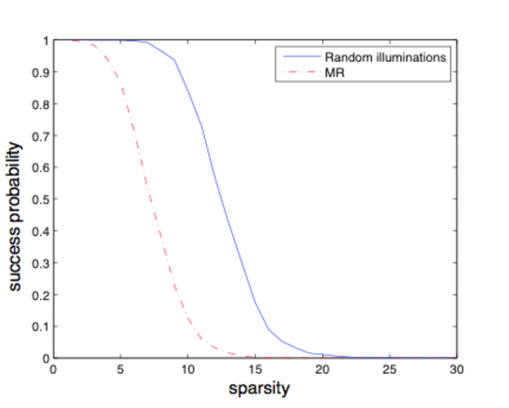
Figure 3. The Lasso performance comparison between RI with $n=11,p=6$ and MR with $n=11$. The vertical axis is for the success probability and the horizontal axis is for the number of objects. The success probability is estimated from 1000 independent trials.

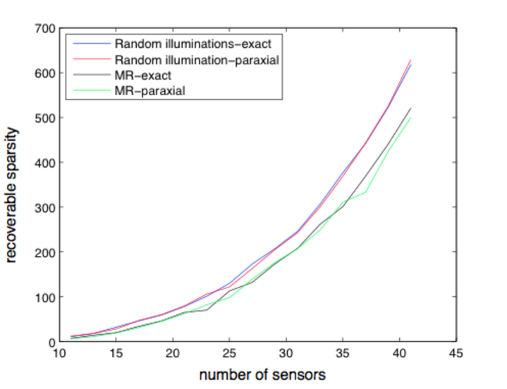
Figure 4. The numbers of recoverable (by the Lasso) objects for RI with $p=(n+1)/2$ and MR as $n$ varies. The curves indicate a quadratic behavior predicted by the theory. The difference between recoveries with the exact and paraxial Green functions is negligible in both the RI and MR set-ups.

We use two numerical settings: the diffraction-limited case when (28) is satisfied (Figure 3, 4, 5, 6) and the under-resolved case when the ratio in (28) is smaller than unity (Figure 7).

For the diffraction-limited case we set $z_{0}=10000$ and $\lambda=0.1$ for the search domain $[-250,250]^{2}$ with $\ell=10$. The targets are i.i.d. uniform random points in the grid with amplitudes in the range $[1,2]$. We randomly select sensor locations from $[-50,50]^{2}$ with the aperture $A=100$ satisfying (28). With these parameters

$${(A+\ell\sqrt{N})^{4}\over\lambda z^{3}_{0}}\approx 1.3$$

the condition (23) is barely satisfied. For the Lasso solution we have used the Matlab code Subspace Pursuit (available at http://igorcarron.googlepages.com/cscodes).

We use the true Green function (20) in the computation of scattered waves and in recovery the exact Green function as well as its paraxial approximation to construct the sensing matrix (for comparison). In other words, we allow model mismatch between the forward and inversion steps.

In the first set of simulations, we compare the performances of the Lasso for two imaging set-ups: one with random illumination (RI) and the other with multi-static responses (MR). As Figure 3 shows, the RI set-up has a higher success probability than the MR set-up. Another comparison is shown in Figure 4 in terms of the number of recoverable objects over a range of $n$. The quadratic behavior is consistent with the prediction of (39) and (36). The difference between the exact and paraxial Green functions recoveries is negligible in both the RI and MR set-ups. For a given $n$, the Lasso with the RI set-up recovers a higher number of objects than does the Lasso with the MR set-up.

Figure 5 compares the performances of the Lasso (top panel) and OST (bottom panel) in terms of the number of recoverable objects for a fixed $np=600$ but variable $n$. Clearly, the Lasso can recover far more objects exactly than does the OST. For a fixed $np$ the performance for each method appears relatively constant over the whole range of $n$. For small $n$, the performance curves of both methods indicate superresolution. As noise level increases the Lasso performance decays (Figure 6).

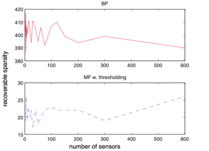
Figure 5. The number of recoverable objects as a function of the number of sensors $n=$ 1,2,3,4,5, 6, 8, 10, 12, 15, 20, 24, 25, 30, 40, 50, 60, 75, 100, 120, 150, 200, 300, 600 with $np=600$ fixed. The top panel is for the Lasso and the bottom panel for OST. The left ends of both curves indicate superresolution.

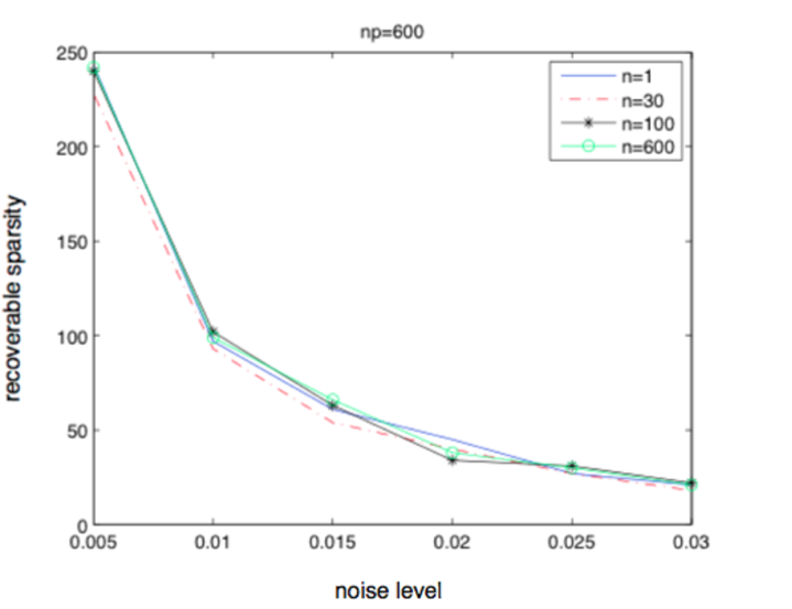
Figure 6. Noisy recovery by the Lasso for $n=1,30,100,600$ and with $np=600$ fixed. The noise is given by the circularly random Gaussian noise of magnitude $\sigma\|Y\|_{2}$ where $\sigma$ is the horizontal coordinate. Note that in this case $\mathbb{E}\|E\|_{2}^{2}=np\sigma^{2}\|Y\|_{2}^{2}.$

To further understand the superresolution effect of random illumination, we consider the set-up with $z_{0}=25000,\lambda=0.4$ for which the ratio in (28) is $0.1$. This is an under-resolved case whose performance is shown in Figure 7. In contrast to the diffraction-limited case (Figure 5), the number of recoverable objects in the under-resolved case decays rapidly as $p$ decreases ($n$ increases). To maintain high performance in the under-resolved case, it is necessary that $p\gg 1$. The number of recoverable objects is calculated based on 90% recovery of 100 independent trials.

We demonstrate in Figures 8- 11 the performance for extended objects in the presence of external noise of the form

$${p\over\sqrt{2}}(\nu_{1}+\imath\nu_{2}){\|Y\|_{2}\over\sqrt{np}},\quad p=5\%,20\%$$

where $p$ is the percentage of noise in each entry of the data vector and $\nu_{1},\nu_{2}$ are i.i.d. uniform random variables in $[0,1]$.

Figure 8 shows the original $40\times 80$ pixel image (left) and its reconstructions (middle panel, $5\%$ noise; right panel, $20\%$ noise) by the BPDN solver YALL1 (http://yall1.blogs.rice.edu/) using one sensor and 500 random illuminations while Figure 9 shows the results with one illuminations and 500 randomly distributed sensors.

Figure 10 shows the original $70\times 70$ pixel image (left), the Shepp-Logan phantom, and its reconstructions (middle panel, $5\%$ noise; right panel, $20\%$ noise) by the total-variation minimization [14, 31] solver TVAL3 (http://www.caam.rice.edu/ optimization/L1/TVAL3/) using one sensor and 1000 random illuminations while Figure 11 shows the results with one illumination and 1000 randomly distributed sensors.

The low pixel numbers are chosen to reduce the run time of the programs.

For the one-illumination reconstructions (Figures 9 and 11), the classical resolution criterion (28) is met. Note, however, that the Shepp-Logan phantom is not in the class of sparse extended objects analyzed in Section 4 because the object support covers more than $50\%$ of the domain (only the gradient is sparse). As a result, the same percentage of noise represents a greater amount of noise in the case of Shepp-Logan phantom and has a more serious effect on performance (Figures 10 and 11, right panels).

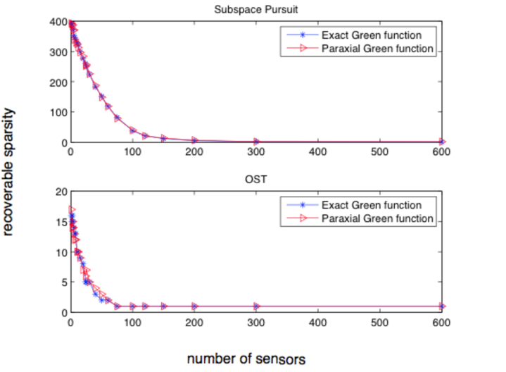
Figure 7. The number of recoverable objects in the under-resolved case as a function of the number of sensors $n=$ 1,2,3,4,5, 6, 8, 10, 12, 15, 20, 24, 25, 30, 40, 50, 60, 75, 100, 120, 150, 200, 300, 600 with $np=600$ fixed.

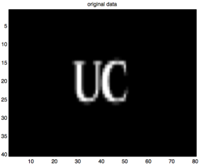
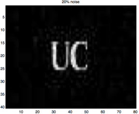
Figure 8. The original $40\times 80$ pixel image (left) and the BPDN reconstructions (middle panel, $5\%$ noise; right panel $20\%$ noise) with one sensor and 500 random illuminations.

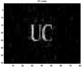
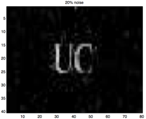
Figure 9. The original $40\times 80$ pixel image (left) and the BPDN reconstructions (middle panel, $5\%$ noise; right panel, $20\%$ noise) with one illumination and 500 randomly distributed sensors.

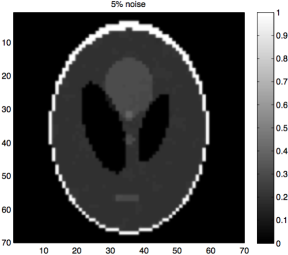
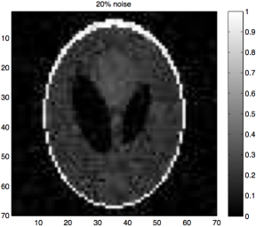
Figure 10. The original $70\times 70$ pixel image (left), the Shepp-Logan phantom, and the TV-minimization reconstructions (middle panel, $5\%$ noise; right panel, $20\%$ noise) with one sensor and 1000 random illuminations.

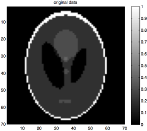
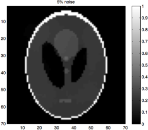
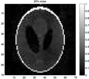
Figure 11. The original $70\times 70$ pixel image (left), the Shepp-Logan phantom, and the TV-minimization reconstructions (middle panel, $5\%$ noise; right panel, $20\%$ noise) with one illumination and 1000 randomly distributed sensors.

9. Conclusion

We have proposed a new approach to superresolving point and extended objects based on random illumination and compressed sensing reconstruction.

We have proved that in the diffraction-limited case both the Lasso and the OST with random illumination can exactly localize $s=\mathcal{O}(m)$ objects where the number of data $m$ is the product of the numbers of random probes and sensors. For the under-resolved case where the Rayleigh resolution limit is broken, the Lasso still has a similar performance guarantee if the number of random illuminations is sufficiently large. It is possible to extend the OST result to the under-resolved case which is omitted here to simplify the presentation.

Numerical evidence supports our theoretical prediction and confirms the superiority of the Lasso to the OST in the set-up with random illumination.

We have also shown that the BPDN is suitable for imaging extended objects and have provided numerical examples to demonstrate its performance.

The superresolution effect with random illumination revealed here contrasts with the subwavelength resolution with deterministic near-field illumination studied in [20].

Finally we note that in our approach it is essential to measure the wave field. For intensity-only measurements, additional techniques such as interferometry or phase retrieval methods are necessary for object reconstruction.

Acknowledgement    I am grateful to Mike Yan for producing Figures 3-7 and Hsiao-Chieh Tseng for producing Figures 8-11 of Section 8.

References

- [1] P. F. Almoro, G. Pedrini, P. N. Gundu, W. Osten, S. G. Hanson, ” Enhanced wavefront reconstruction by random phase modulation with a phase diffuser,” Opt. Laser Eng. 49 (2011) 252-257.
- [2] A.B. Baggeroer, W.A. Kuperman and P.N. Mikhalevsky, ”An overview of matched field methods in ocean acoustics”, IEEE J. Oceanic Eng.18 (1993), 401-424.
- [3] W.U. Bajwa, R. Calderbank and S. Jafarpour, “Model selection: Two fundamental measures of coherence and their algorithmic significance,” arXiv: 0911.2746v2. To appear in Proceedings of IEEE International Symposium on Information Theory, 2010.
- [4] R. Baraniuk, M. Davenport, R. DeVore and M. Wakin, “A Simple proof of the restricted isometry property for random matrices,” Constr. Approx. 28 (2008), 253-263.
- [5] A. Barron, L. Birgé, and P. Massart, “ Risk bounds for model selection via penalization,” Probab. Theory Related Fields 113 (1999), 301 413.
- [6] L. Birgé and P. Massart, “ Gaussian model selection,” J. Eur. Math. Soc. (JEMS) 3(3) (2001), 203 268.
- [7] D. J. Brady, K. Choi, D. L. Marks, R. Horisaki, and S. Lim, “Compressive holography,” Opt. Exp. 17 (2009), 13040-13049.
- [8] R. Bräuer, U. Wojak, F. Wyrowski, O. Bryngdahl, ” Digital diffusers for optical holography,” Opt Lett 16 (1991):1427 9.
- [9] A.M. Bruckstein, D.L. Donoho and M. Elad, “From sparse solutions of systems of equations to sparse modeling of signals,” SIAM Rev. 51 (2009), 34-81.
- [10] F. Bunea, A. B. Tsybakov, and M. H. Wegkamp, “ Sparsity oracle inequalities for the Lasso,” Electron. J. Stat. 1 (2007), 169 194.
- [11] E. J. Candès, “The restricted isometry property and its implications for compressed sensing,” Compte Rendus de l’Academie des Sciences, Paris, Serie I. 346 (2008) 589-592.
- [12] E.J. Cand‘es and Y. Plan, Near-ideal model selection by l1 minimization, Ann. Statist. 37 (2009), 2145-2177.
- [13] E. J. Candès and T. Tao, “ Decoding by linear programming,” IEEE Trans. Inform. Theory 51 (2005), 4203 4215.
- [14] A. Chambolle and P.-L. Lions ”Image recovery via total variation minimization and related problems, ” Numer. Math. 76 (1997), 167-188.
- [15] S.S. Chen, D.L. Donoho and M.A. Saunders, “Atomic decomposition by basis pursuit,” SIAM J. on Sci. Comp.20 (1998), 33 61.
- [16] W. Dai and O. Milenkovic, “Subspace pursuit for compressive sensing: closing the gap between performance and complexity,” arXiv:0803.0811.
- [17] P. Delsarte, J. M. Goethals, and J. J. Seidel, Bounds for systems of lines and Jacobi poynomials, Philips Res. Repts. 30:3 pp. 91 105, 1975, issue in honour of C.J. Bouwkamp.
- [18] D.L. Donoho, M. Elad and V.N. Temlyakov, “Stable recovery of sparse overcomplete representations in the presence of noise,” IEEE Trans. Inform. Theory 52 (2006) 6-18.
- [19] M. Duarte, M. Davenport, D. Takhar, J. Laska, T. Sun, K. Kelly, and R. Baraniuk, “Single-pixel imaging via compressive sampling,” IEEE Sig. Proc. Mag. 25(2) (2008), 83 - 91.
- [20] A.C. Fannjiang, “Compressive imaging of subwavelength structures,” SIAM J. Imag. Sci. 2 (2009), 1277-1291.
- [21] A.C. Fannjiang, “Compressive inverse scattering I. High-frequency SIMO/MISO and MIMO measurements,” Inverse Problems 26 (2010), 035008.
- [22] A.C. Fannjiang, “The MUSIC algorithm for sparse objects: a compressed sensing analysis,” arXiv: 1006.1678.
- [23] A. Fannjiang and K. Solna, “Broadband Resolution Analysis for Imaging with Measurement Noise,” J. Opt. Soc. Am. A 24 (2007), 1623-1632
- [24] A. Fannjiang, P. Yan and Thomas Strohmer, “Compressed remote sensing of sparse objects,” SIAM J. Imag. Sci., in press.
- [25] W. Feller, An Introduction to Probability Theory and its Applications. volumn II, 2nd edition, New York: John Wiley and Sons, 1970.
- [26] E. Greenshtein, “ Best subset selection, persistence in high-dimensional statistical learning and optimiza- tion under - constraint, ” Ann. Statist. 34(5) (2006), 2367 2386.
- [27] W. Hoeffding, “Probability inequalities for sums of bounded random variables”, J. Amer. Stat. Assoc. 58 (1963) 13 30.
- [28] N. Meinshausen and P. Bühlmann, “High-dimensional graphs and variable selection with the lasso, ” Ann. Statist. 34(3) (2006), 1436 1462.
- [29] H. Rauhut, “Stability results for random sampling of sparse trigonometric polynomials,” IEEE Trans. Inform. Th. 54 (2008), 5661-5670.
- [30] J. Romberg, “Compressive sensing by random convolution,” SIAM J. Imaging Sci. 2 (2009), 1098-1128.
- [31] L.I. Rudin, S. Osher and E. Fatemi, ” Nonlinear total variation based noise removal algorithms,” Physica D 60 (1992) 259-268.
- [32] V. V. Senatov, Normal Approximation: New Results, Methods, and Problems, Utrecht, The Netherlands, 1998.
- [33] M. Shahram and P. Milanfar, Imaging below the diffraction limit: a statistical analysis, IEEE Trans. Image Proc. 13 (2004), 677 689.
- [34] T. Shirai and E. Wolf, ”Coherence and polarization of electromagnetic beams modulated by random phase screens and their changes on propagation in free space,” JOSA A 21 (2004), 1907-1916.
- [35] R. Tibshirani, “Regression shrinkage and selection via the lasso,” J. Roy. Statist. Soc. Ser. B 58 (1996), 267-288.
- [36] A. Tolstoy, Matched Field Processing in Underwater Acoustics, World Scientific, Singapore, 1993.
- [37] J.A. Tropp, “Greed is good: algorithmic results for sparse approximation,” IEEE Trans. Inform. Theory 50 (2004), 2231-2242.
- [38] J.A. Tropp, “ Just relax: convex programming methods for identifying sparse signals in noise,” IEEE Trans. Inform. Theory 52 (2006), 1030 -1051. “Corrigendum” IEEE Trans. Inform. Theory (2008).
- [39] J.A. Tropp, “On the conditioning of random subdictionaries,” Appl. Comput. Harmon. Anal. 25 (2008), 1 - 24.
- [40] L. Welch, Lower bounds on the maximum cross-correlation of signals, IEEE Trans. on Information Theory, 20 (1974), pp. 397 - 399.
- [41] P. Zhao and B. Yu, “On model selection consistency of Lasso,” J. Mach. Learn. Res. 7 (2006), 2541 - 2563.