On a class of distributions stable under random summation

Abstract

We investigate a family of distributions having a property of stability-under-addition, provided that the number $\nu$ of added-up random variables in the random sum is also a random variable. We call the corresponding property a  $\nu$-stability and investigate the situation with the semigroup generated by the generating function of $\nu$ is commutative.

Using results from the theory of iterations of analytic functions, we show that the characteristic function of such a $\nu$-stable distribution can be represented in terms of Chebyshev polynomials, and for the case of $\nu$-normal distribution, the resulting characteristic function corresponds to the hyperbolic secant distribution.

We discuss some specific properties of the class and present particular examples.

Key Words: Stability, random summation, characteristic function, hyperbolic secant distribution.

1 Introduction

In many applications of probability theory certain specific classes of distributions have become very useful, usually called ”fat tailed” of ”heavy tailed” distributions. The Stable distributions that originate from the Central Limit problem, are probably most popular among the heavy tailed distributions, however there is a wide collection of classes of distributions, all related to Stable ones in many various ways, often these relations are not at all obvious.

Besides, certain generalizations of stable distributions are known, using sums of random numbers of random variables (instead of sums with deterministic number of summands), see e.g. Gnedenko [3], Klebanov, Mania, Melamed [8], for the examples of such, including the so-called $\nu$-stable distributions, introduced independently by Klebanov and Rachev [9] and Bunge [1].

In the present paper, we focuse on presenting further examples of strictly $\nu$-stable random variables, that could be useful in practical applications, including applications in financial mathematics.

2 Definition of strictly $\nu$-stable r.v.’s, properties and examples

In the present section, we give a general insight on strictly $\nu$-stable distributions and describe some examples that have been mentioned in the literature before.

2.1 Basic definitions

Let $X,X_{1},X_{2},\dots,X_{n},\dots$ be a sequence of i.i.d. random variables, and let $\{\,\nu_{p}\,,\,p\in\Delta\,\}$ be a family of some discrete r.v.’s taking values in the set of natural numbers $\mathbb{N}$. Assume that this family does not depend on the sequence $\{X_{j},\,j\geq 1\}$, and that, for $\Delta\subset(0,1)$,

$$\mathbf{E}\,\left[\,\nu_{p}\,\right]=\frac{1}{p}\,,\,\,\,\forall\,p\in\Delta\,.$$ (1)

Definition 2.1.

We say that the r.v. $X$ has a strictly $\nu$–stable distribution, if   $\forall\,\,p\in\Delta$ it holds that

$$X\overset{d}{=}p^{1/\alpha}\sum_{i=1}^{\nu_{p}}X_{j}\,,$$

where $\alpha\in(0,2]$ is called the index of stability.

After this general definition, a narrower class is defined for $\alpha=1/2$.

Definition 2.2.

We call the r.v. $X$ a strictly $\nu$–normal r.v., if   $\mathbf{E}X=0$, $\mathbf{E}X^{2}=\infty$, and the following holds:

$$X\overset{d}{=}p^{1/2}\sum_{i=1}^{\nu_{p}}X_{j}\,,\,\,\,\,\forall\,\,p\in\Delta\,\,.$$

Closely related to the stability property is the property of infinite divisibility, so we also give the following definition.

Definition 2.3.

$X$ has a strictly $\nu$–infinitely divisible distribution, if for any $p\in\Delta$, there exists a r.v. $Y^{(p)}$, s.t.

$$X\overset{d}{=}\sum_{j=1}^{\nu_{p}}Y^{(p)}_{j}\,,\,\,\,\,\mbox{with}\,\,Y^{(p)},Y^{(p)}_{1},\dots,Y^{(p)}_{n},\dots\,\,\mbox{being iid r.v.'s}\,\,.$$

A powerful tool for investigating distributions’ properties is the generating function. We shall use the generating function of the r.v. $\nu_{p}$   denoting it by $\mathcal{P}_{p}(z):=\mathbf{E}\left[z^{\nu_{p}}\right]$. Moreover, we denote by $\mathcal{A}$ the semigroup generated by the family $\{\,\mathcal{P}_{p}\,,\,\,p\in\Delta\}$, with the operation of the functions’ composition.

2.2 Summary of the known results

With regards to the definitions above, the following results are known (see e.g. [7] for proofs and details).

Theorem 2.1.

For the family $\{\,\mathcal{P}_{p}\,,\,\,p\in\Delta\}$, with   $\mathbf{E}\left[\nu_{p}\right]=\frac{1}{p}$ ,   there exists a strictly $\nu$-normal distribution, iff   the semigroup $\mathcal{A}$ is commutative.

Suppose that we have a commutative semigroup $\mathcal{A}$. Then the following statements (that we refer to in the sequel as Properties) are known to be true (see [7] for proofs and details):

1. The system

   $$\varphi(t)=\mathcal{P}_{p}(\varphi(pt)),\,\,\,\forall\,p\in\Delta\,.$$ (2)

   of functional equations has a solution that satisfies the initial conditions

   $$\varphi(0)=1\,,\,\,\,\varphi^{\prime}(0)=-1\,.$$ (3)

   The solution is unique. In addition, there exists a distribution function (cdf) $A(x)$   (with $A(0)=0$) such that

   $$\varphi(t)=\int\limits_{0}^{\infty}e^{-tx}dA(x).$$ (4)

2. The characteristic function (ch.f.) of the strictly $\nu$-normal distribution has the form

   $$f(t)=\varphi(at^{2})\,,\,\,\,\,a>0\,.$$ (5)

3. A ch.f. $g(t)$ is a ch.f. of a $\nu$-infinitely divisible r.v., iff there exists a chf $h(t)$ of an infinitely divisible (in the usual sense) r.v., such that

   $$f(t)=\varphi(-\ln h(t)).$$ (6)

The relation (6) allows obtaining explicit representations of ch.f. of strictly $\nu$-stable distributions. Clearly, they are obtained through applying (6) to a ch.f.  $h(t)$ , provided that the r.v. corresponding to  $h(t)$  is strictly stable (in the usual sense). Moreover, note that the ch.f. $\varphi(ait)$,  $a\in\mathbb{R}^{1}$, is the ch.f. of an analogue of the degenerate r.v., and that for the r.v. with such ch.f. the following analogue of the Law of Large Numbers exists.

Theorem 2.2.

Let $X_{1},X_{2},\dots,X_{n},\dots$ be a sequence of iid random variables with the finite absolute value of the first moment, and $\{\,\nu_{p}\,,\,p\in\Delta\,\}$ a family of r.v.’s taking values in $\mathbb{N}$, independent of the sequence $\{X_{j},j=1,2,\dots\}$. Assume that $\mathbf{E}\left[\nu_{p}\right]=\frac{1}{p}$ and that the semigroup $\mathcal{A}$ is commutative.

Then the series $p\sum\limits_{j=1}^{\nu_{p}}X_{j}$ is convergent is distribution, as $p\rightarrow 0$, and the limit of convergence is a r.v. having the ch.f.   $\varphi(ait)$.

The proof of this theorem follows straightforwardly from the Property 1 outlined above and from the Transfer Theorem of Gnedenko, see e.g. [4].

In the following paragraph we discuss several particular examples of strictly $\nu$-normal and strictly $\nu$-stable distributions.

2.3 Examples and the outline of the problem

Example 1 .  The usual stability.
Assume the following setup :   $\nu_{p}=\frac{1}{p}$   with probability $1$, where $p\in\Delta=\left\{1,\frac{1}{2},\dots,\frac{1}{n},\dots\right\}$ , and so $\mathcal{P}_{p}(z)=z^{1/p}$ .

Clearly, the corresponding semigroup $\mathcal{A}$ is commutative.

Furthermore, $\varphi(t)=\exp\{-t\}=\int\limits_{0}^{\infty}e^{-tx}dA(x)$, where $A(x)$ is a cdf with a single unit-sized jump at $x=1$. In this setup the strictly $\nu$-normal ch.f. is the ch.f. of the normal (in the usual sense) r.v. with the zero mean.

Example 2 . The geometric summation scheme.
Suppose, $\nu_{p}$ is the r.v. having a geometric distribution

$$\mathbf{P}\{\nu_{p}=k\}=p(1-p)^{k-1}\,,\,\,\,k=1,2,\dots\,\,\,,\,p\in(0,1)\,.$$

Clearly, here $\mathbf{E}\left[\nu_{p}\right]=\frac{1}{p}$ ,  and $\mathcal{P}_{p}(z)=\frac{pz}{1-(1-p)z}$ ,  $p\in(0,1)$ . It is quite straightforward to check that $\mathcal{A}$ is commutative.

Moreover, a direct calculation gives $\varphi(t)=\frac{1}{1+t}=\int\limits_{0}^{\infty}e^{-tx}e^{-x}dx$, i.e. $A(x)$ is the cdf of the exponential distribution. So that a $\nu$-analogue of the strictly normal distribution is the Laplace distribution with the ch.f.  $f(t)=\frac{1}{1+at^{2}}$  .

Example 3 . Branching process scheme.
Let $\mathcal{P}(z)$ be some generating function, with $\mathcal{P}^{\prime}(1)=\frac{1}{p_{0}}>1$ (so that the introduced notation is $p_{0}=1/\mathcal{P}^{\prime}(1)$, with the condition $p_{0}<1$).

Consider now a family given by $\mathcal{P}^{0\,n}(z)=\mathcal{P}^{0(n-1)}\left(\mathcal{P}(z)\right)$ ,  $n=1,2,\dots$ . Related to that is another family of the r.v.’s $\nu_{p}$ :  $\mathcal{P}_{p}(z)=\mathcal{P}^{0\,n}(z)\,,\,\,p\in\left\{\frac{1}{p_{0}^{n}}\,,\,\,n=1,2,\dots\right\}=:\Delta$ .

Clearly, the semigroup $\mathcal{A}$ coincides with the family $\{\mathcal{P}_{p}\,,\,\,p\in\Delta\}$ .  The ch.f. $\varphi(t)$ is a solution of the functional equation $\varphi(t)=\mathcal{P}\left(\varphi(p_{0}t)\right)$  .

It can be noted that the content of the paper by Mallows and Shepp [11] is actually based on considering an example identical to the Example 3 above. Probably, neither the authors of that work nor its reviewers were familiar with the works by Klebanov and Rachev [9] and Bunge [1], which had dealt with exactly the same example a number of years earlier.

Like mentioned in Introduction, in the present work we aim in widening the collection of examples that involve random summation with the commutative semigroup $\mathcal{A}$. For that purpose, we address the description of pairs of certain commutative generating functions $\mathcal{P}$ and $\mathcal{Q}$, i.e. the ones for which the balance equality $\mathcal{P}\circ\mathcal{Q}=\mathcal{Q}\circ\mathcal{P}$ holds, – but including only the case when there exists no such function $\mathcal{H}$ such that $\mathcal{P}=\mathcal{H}^{0k}$ and $\mathcal{Q}=\mathcal{H}^{0m}$  for some $k,m\in\mathbb{N}$  (which would be exactly the case of the Example 3).

In a general setting, the problem of describing all such commutative pairs of generating functions appears, unfortunately, far too involved to approach. However, certain special cases are rather straightforward for consideration. In order to approach the problem, we will use certain notions typical for the theory of iterations of analytic functions, that we outline in the separate section below.

3 Theoretic justification via iterations of analytic functions

Let $\mathcal{P}$ be a rational function with $(\deg)\geq 2$. Denote by $\mathcal{P}^{0n}$ its $n$th iteration. The functions $\mathcal{P}$ and $\mathcal{Q}$ are called conjugates, if there exists a linear-fractional function $R$, such that $\mathcal{P}\circ R=R\circ\mathcal{Q}$ .

A subset $E$ of the extended complex plane $\overline{\mathbb{C}}$ is called completely invariant, if its complete inverse image $\mathcal{P}^{-1}(E)$ coincides with $E$. The maximal finite completely invariant set $E(\mathcal{P})$ exists and is called the exceptional set of the function $\mathcal{P}$ . It is always the case that $\mbox{card}\,E(\mathcal{P})\leq 2$ . Moreover, if $\mbox{card}\,E(\mathcal{P})=1$ then the function $\mathcal{P}$ is a conjugate to a polynomial, while for $\mbox{card}\,E(\mathcal{P})=2$ the function $\mathcal{P}$ is a conjugate to $\mathcal{Q}(z)=z^{n}\,,\,\,n\in\mathbb{Z}\backslash\{0,1\}$ . Clearly, $E(\mathcal{Q})=\{0,\infty\}$.

If $\mathcal{P}$ is a rational function, then it is known (see e.g. [7]) that there is a finite number of open sets $F_{i}$ ,   $i=1,\dots,r$ ,  which are left invariant by the operator $\mathcal{P}$ and are such that (in the sequel, we will refer to the two points below as Conditions)

1. the union $\bigcup\limits_{i=1}^{r}F_{i}$ is dense on the plane ;

2. and $\mathcal{P}$ behaves regularly and in a unique way on each of the sets $F_{i}$ .

The latter means that the termini of the sequences of iterations generated by the points of $F_{j}$ are either precisely the same set, which is then a finite cycle, or they are finite cycles of finite or annular shaped sets that are lying concentrically. In the first case the cycle is attracting, in the second one it is neutral.

The sets $F_{j}$ are the Fatou domains of $\mathcal{P}$, and their union is the Fatou set  $F(\mathcal{P})$ of $\mathcal{P}$.

The complement of $F(\mathcal{P})$ is the Julia set  $\mathcal{J}(\mathcal{P})$ of $\mathcal{P}$ . Note that $\mathcal{J}(\mathcal{P})$ is either a nowhere dense set (that is, without interior points) and an uncountable set (of the same cardinality as the real numbers), or $\mathcal{J}(\mathcal{P})=\overline{\mathbb{C}}$ . Like $F(\mathcal{P})$, $\mathcal{J}(\mathcal{P})$ is left invariant by $\mathcal{P}$, and on this set the iteration is repelling, meaning that $\,\,|\,\mathcal{P}(z)-\mathcal{P}(w)\,|\,>\,|\,z-w\,|\,\,$ for all elements $w$ in a neighborhood of $z$ (within $\mathcal{J}(\mathcal{P})$). This means that $\mathcal{P}(z)$ behaves chaotically on the Julia set. Although there are points in the Julia set whose sequence of iterations is finite, there is only a countable number of such points (and they make up an infinitely small part of the Julia set). The sequences generated by points outside this set behave chaotically, a phenomenon called deterministic chaos. Let $z_{0}$ be a repelling fixed point of the function $\mathcal{P}$, and let $\lambda=\mathcal{P}^{\prime}(z_{0})$. Define $\Lambda\,:\,\,z\rightarrow\lambda z$ . Then there exists a unique solution of the Poincaré equation

$$F\circ\Lambda=\mathcal{P}\circ F\,,\,\,\,\,F(0)=z_{0}\,,\,\,\,F^{\prime}(0)=1\,,$$

that is meromorphic in $\overline{\mathbb{C}}$ .

Now let

$$\mathcal{I}(\mathcal{P})=F^{-1}(\mathcal{J}(\mathcal{P}))\,.$$

If for two functions $\mathcal{P}$ and $\mathcal{Q}$ we have $\mathcal{P}\circ\mathcal{Q}=\mathcal{Q}\circ\mathcal{P}$, then they have the same function $F$.

There are the two following possibilities:

1. $\mathcal{I}(\mathcal{P})=\mathbb{C}$ ,  in which case $\mathcal{J}(\mathcal{P})=\overline{\mathbb{C}}$,.

2. $\mathcal{I}(\mathcal{P})$ is nowhere dense and consists of analytic cuvrves.

Fatou  [2], and Julia  [5] investigated the case. It turned out that is this case $\mathcal{P}$ and $\mathcal{Q}$ can be reduced by a conjugancy either to the form $\mathcal{P}(z)=z^{m}$ and $\mathcal{Q}(z)=z^{n}$ or to the form $\mathcal{P}(z)=T_{m}(z)$ and $\mathcal{Q}(z)=T_{n}(z)$ , where $T_{k}$ is the Chebyshev polynomial determined by the equation  $\cos(k\zeta)=T_{k}(\cos\zeta)$.

4 Main results

4.1 A new example

Let us return to the study of $\nu$-normal and $\nu$-stable random variables. Recall that we deal with the family $\{\nu_{p}\,,\,\,p\in\Delta\}$ taking its values in $\mathbb{N}=\{1,2,\dots\}$ . As before, we work with the generating function ,  $\mathcal{P}_{p}(z)=\mathbf{E}\left[\,z^{\nu_{p}}\,\right]$ , of $\nu_{p}$ . The important result that we stressed says the a strictly $\nu$-normal (resp. strictly $\nu$-stable) r.v. exist iff the semigroup $\mathcal{A}$ generated by $\{\mathcal{P}_{p}\,,\,\,p\in\Delta\}$   is commutative. If $\mathcal{P}_{p}\,,\,\,p\in\Delta$ ,  is a rational function (with $\deg\leq 2$) satisfying Condition 2  of the above section, then either $\mathcal{P}_{p}(z)$ is reduced to a form $\widetilde{\mathcal{P}}_{p}(z)=z^{1/p}$ ,  $p\in\left\{\frac{1}{n}\,,\,n=1,2,\dots\right\}$, and then we deal, in fact, with the classical (deterministic) summation scheme, or $\mathcal{P}_{p}(z)$ is reduced to the form $\mathcal{P}_{p}(z)=T_{1/\sqrt{p}}(z)$ ,  $p\in\left\{\frac{1}{n^{2}}\,,\,n=1,2,\dots\right\}$ . Clearly, the polynomial $T_{m}(z)$ is not a generating function itself, however a function to which it is a conjugate, specifically the function

$$\mathcal{P}_{p}(z)=\frac{1}{T_{1/\sqrt{p}}(z)}\,\,,\,\,\,p\in\left\{\frac{1}{n^{2}}\,,\,n=1,2,\dots\right\}\,\,,$$ (7)

is indeed a generating function, – the fact that we prove below. Moreover, below we consider in some details a family of r.v.’s $\left\{\nu_{p}\,,\,p\in\left\{\frac{1}{n}\,,\,n=1,2,\dots\right\}\,\right\}$ that have generating functions of the form (7), and investigate the corresponding strictly $\nu$-normal and strictly $\nu$-stable distributions.

Lemma 4.1.

Let $P_{n}(x)$ be a polynomial with  $\deg P_{n}=k$   by the even powers of $x$, and whose zeros are all within the interval $(-1,1)$ .  Let  $P_{n}(1)=1$ and polynomial’s coefficient with with $x^{n}$ be positive. Then for any natural number $k$, the function

$$\mathcal{P}(x)=\frac{x^{k}}{P_{n}(\frac{1}{x})}$$

is a generating function.

Proof.

Represent $P_{n}(x)$ as

$$P_{n}(x)=b_{0}+b_{1}x+\dots+b_{n}x^{n}=b_{n}\prod\limits_{j=1}^{n}\left(x-a_{j}\right)\,,$$

where $a_{j}$  ($j=1,\dots,n$)  are the zeros of the polynomial $P_{n}$   sorted in the order of ascendance. As $P_{n}$ is a polynomial by the even powers of $x$, then, if $a_{j}$ is a zero of $P_{n}$, then $-a_{j}$ is also a zero of $P_{n}$. Therefore,

$$\frac{1}{P_{n}(\frac{1}{x})} = \frac{1}{b_{n}\prod\limits_{j=1}^{n}\left(\frac{1}{x}-a_{j}\right)}$$ (8)

$$= \frac{1}{b_{n}\prod\limits_{j=1}^{n/2}\left(\frac{1}{x}-a_{j}\right)\left(\frac{1}{x}+a_{j}\right)}$$

$$= \frac{1}{b_{n}}\prod\limits_{j=1}^{n/2}\frac{1}{\left(\frac{1}{x}-a_{j}\right)\left(\frac{1}{x}+a_{j}\right)}$$

$$= \frac{1}{b_{n}}\prod\limits_{j=1}^{n/2}\frac{x^{2}}{1-a_{j}^{2}x^{2}}$$

Obviously,

$$\frac{x^{2}}{1-a_{j}^{2}x^{2}}=\sum\limits_{k=0}^{\infty}a^{2k}_{j}x^{2k+2}$$

is a series with positive (non-negative) coefficients, converging when $|x|\leq 1$. From (8), it now follows that  $\mathcal{P}(x)=\frac{x^{k}}{P_{n}(\frac{1}{x})}$  is a series also convergent when $|x|\leq 1$, having non-negative coefficients, and $\mathcal{P}(1)=1$ . Hence, $\mathcal{P}(x)$ is a generating function of some random variable. ∎

Corrolary 4.1.

Let $T_{n}(x)$ be a Chebyshev polynomial of degree $n$. Then

$$\mathcal{P}(x)=\frac{1}{T_{n}(\frac{1}{x})}$$

is a generating function of some r.v. taking values in $\mathbb{N}$.

Proof.

When $n$ is an even number, the result follows directly from Lemma 4.1 and from the properties of Chebyshev polynomials. For odd $n$, consider the representation
$T_{n}(x)=xP_{n-1}(x)$, where $P_{n-1}(x)$ is a polynomial by the even degrees of $x$, satisfying the conditions of Lemma 4.1. ∎

Let us now set $\Delta:=\left\{\frac{1}{n^{2}}\,,\,n=1,2,\dots\right\}$ .  Consider the family of generating functions

$$\mathcal{P}_{p}(z)=\frac{1}{T_{1/\sqrt{p}}(1/z)}\,,\,\,\,\,p\in\Delta\,.$$

Clearly,    $\mathcal{P}_{p_{1}}\circ\mathcal{P}_{p_{2}}=\mathcal{P}_{p_{2}}\circ\mathcal{P}_{p_{1}}$   for all $p_{1},p_{2}\in\Delta\,$ , due to the well known property of Chebyshev polynomials stating that  $T_{n}(T_{m}(x))=T_{n\cdot m}(x)$.  In other words, semigroup generated by the family $\{\,\mathcal{P}_{p}\,,\,\,p\in\Delta\}$ is commutative. It follows (see e.g. [7]) that there exists a solution to the system of equations

$$\varphi(t)=\mathcal{P}_{p}(\varphi(pt))\,\,,\,\,\,p\in\Delta\,,$$ (9)

satisfying initial conditions

$$\varphi(0)=1\,\,,\,\,\,\varphi^{\prime}(0)=-1\,,$$ (10)

and the solution is unique.

Since $T_{n}(x)=\cos(n\cdot\arccos x)=\cosh(n\cdot\mbox{arccosh}\,x)$ , the direct plugging gives that the function

$$\varphi(t)=1/\cosh\left(\sqrt{2t}\right)$$ (11)

satisfies the system (9), as well as the conditions (10). Hence, the function

$$f(t)=\frac{1}{\cosh(at)}\,,\,\,\,a>0$$ (12)

is actually a ch.f. of a strictly $\nu$-normal r.v.. The ch.f. (12) is, in fact, well known – it is the ch.f. of the hyperbolic secant distribution. Clearly, here  $a$  is the scale parameter. When $a=1$, it is the case of the standard hyperbolic secant distribution, whose pdf has the form

$$p(x)=\frac{1}{2}\,\mbox{sech}\,\left(\frac{\pi x}{2}\right)\,,$$

while the cdf is

$$F(x)=\frac{2}{\pi}\,\mbox{arctan}\,\left[\exp\left(\frac{\pi x}{2}\right)\right]\,.$$

Furthermore, in order to obtain the expression for the ch.f. of strictly $\nu$-stable distributions, one just needs to apply the relation (6) to the strictly stable (in the usual sense) ch.f. $h$.

4.2 An interesting property

Note that the function $\varphi$, as represented by (11), can be viewed somewhat interesting on its own, and so we shall address its properties and consider its cdf $A(x)$ (which corresponds to $\varphi(t)$ via (4)  ) .

Let $W_{1}(t)$ and $W_{2}(t)$ ,  $t\geq 0$ ,  be two independent Wiener processes. Consider a r.v.

$$\xi=\int\limits_{0}^{1}W_{1}^{2}(t)dt+\int\limits_{0}^{1}W_{2}^{2}(t)dt\,.$$ (13)

This r.v. is well studied, and it is known (see e.g. [12]) that its Laplace transform equals to

$$\mathbf{E}\,\left[\,e^{-t\xi}\,\right]=\frac{1}{\cosh\left(\sqrt{2t}\right)}\,,$$

which coincides with $\varphi(t)$ as given by (11).

Hence $A(x)$ is the cdf of the r.v. $\xi$. On the other hand, as follows from Gnedenko’s Transfer Theorem,

$$A(x)=\underset{p\rightarrow 0}{\lim}\,\,\mathbf{P}\,\{\,p\,\nu_{p}<x\,\}\,\,.$$

Consequently, the following theorem is valid.

Theorem 4.1.

Let $\left\{\,\nu_{p}<x\,,\,\,p\in\Delta\,\right\}$ be a family of r.v.’s having generating functions

$$\mathcal{P}_{p}(z)=\frac{1}{T_{1/\sqrt{p}}(\frac{1}{z})}\,,\,\,\,\,p\in\Delta=\left\{\frac{1}{n^{2}}\,,\,n=1,2,\dots\right\}\,.$$

Then

$$\underset{p\rightarrow 0}{\lim}\,\,\mathbf{P}\,\{\,p\,\nu_{p}<x\,\}=\mathbf{P}\{\xi<x\}\,,$$

where the r.v. $\xi$ is the one defined via (13) .

Theorem 4.1 may be reformulated in the following way.

Let

$$\frac{1}{T_{n}(\frac{1}{z})}=\sum_{k=0}^{\infty}p_{k}(n)z^{k}.$$

Then

$$\lim_{n\to\infty}\sum_{k=0}^{[n^{2}x]}p_{k}(n)=\mathbf{P}\{\xi<x\}.$$

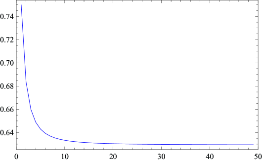
Figure 1: Plot of the $\sum_{k=0}^{[n^{2}x]}p_{k}(n)$ as the function of $n=2,\ldots,50$

On Figure 1, the plot of the $\sum_{k=0}^{[n^{2}x]}p_{k}(n)$ is given as a function of $n$ starting with $n=2$ until $n=50$. We see that the functions attains the constant level rather quickly, and therefore it is possible to use the asymptotic result for $n>25$.

Corrolary 4.2.

Let $X$ be a r.v. having the standard hyperbolic secant distribution. Then its distribution can be represented in the form of a scale mixture of a normal distribution with zero mean and standard deviation $\sqrt{\xi}$, where $\xi$ is defined via (13) .

To prove the above, one just needs to write the ch.f. of $X$ in the form $\int\limits_{0}^{\infty}e^{-t^{2}x}dA(x)$ ,  and note that $e^{-t^{2}x}$ is actually the ch.f. of the standard Normal r.v. $N(0,\sigma^{2})$  ($\sigma^{2}=x$), while $A(x)$ is the cdf of $\xi$ .

Note that there is a certain analogy between the representation $A(x)$ as the cdf of the r.v. $\xi$ from (13) and the corresponding result in the scheme of the random summation with geometric distribution (see e.g. [7]). Specifically, considering the family $\left\{\nu_{p}\,,\,\,p\in(0,1)\right\}$ having the geometric distribution $\mathbf{P}\,\{\,\nu_{p}=k\,\}=p(1-p)^{k-1}$ ,  $k=1,2,\dots$ , the function   $\varphi$   turns into

$$\varphi(t)=\frac{1}{1+t}=\int\limits_{0}^{\infty}e^{-tx}dA_{1}(x)\,,$$

where $A_{1}(x)$ is the cdf of the exponential distribution,  i.e.   $A_{1}(x)=1-e^{-x}$  for  $x>0$   and $A_{1}=0$  for  $x\leq 0$ . It can be checked that if $\eta_{1}$ and $\eta_{2}$ are two independent standard Normal r.v.’s, then $A_{1}$ is a cdf of the r.v.   $\xi_{1}=\eta^{2}_{1}+\eta^{2}_{2}$  ,  which is, in a way, related to (13).

4.3 Characterizations

Let us now turn to the characterizations of the distribution of the r.v. (13) and of the hyperbolic secant distribution.

Theorem 4.2.

Let $X_{1},\dots,X_{n},\dots$ be a sequence of non-negative iid random variables, and $\nu_{p}\,,\,\,p\in\left\{\frac{1}{n^{2}}\,,\,n=2,\dots\right\}$ , is a family of the r.v.’s having the generating function   $\mathcal{P}_{p}(z)=\frac{1}{T_{1/\sqrt{p}}(\frac{1}{z})}$ ,  independent of the sequence   $\{X_{j}\,,\,\,j\geq 1\}$ .

If, for some fixed $p\in\Delta$ ,

$$X_{1}\overset{d}{=}\,p\sum\limits_{j=1}^{\nu_{p}}X_{j}\,\,,$$ (14)

(where ”$\overset{d}{=}$” is the equality in distribution), then $X_{1}$ has the distribution whose Laplace transform is

$$\mathbf{E}\left[\,e^{-tX}\,\right]=\frac{1}{\cosh\left(\sqrt{at}\right)}\,,\,\,a>0\,.$$ (15)

Proof.

The equality (14), in terms of the Laplace transform $\Psi(t)=\mathbf{E}\,e^{-tX}$ ,  can be represented as

$$\Psi(t)=\mathcal{P}_{p}\left(\Psi(pt)\right)\,.$$ (16)

Clearly, the function

$$\Psi_{a}(t)=\frac{1}{\cosh\left(\sqrt{at}\right)}$$

satisfies (16) for any $a>0$ and, moreover, is analytic in the strip $\,|\,t\,|\,<r$  ( $r>0$ ) .

In the following, we use the results of the book by Kakosyan, Klebanov and Melamed [6]. Example 1.3.2 of this book shows that $\{\,\Psi_{a}\,,\,\,a>0\,\}$ forms a strongly $\varepsilon$-positive family, where $\varepsilon$ is a set of restrictions of Laplace transforms of probability distributions given in $R_{+}$ on an interval  $[0,T]$  $(0<T<r)$ .

Clearly, the operator   $A\,:\,f\,\rightarrow\,\mathcal{P}_{p}(f(pt))$ on $\varepsilon$ is intensively monotone.

The result follows from Theorem 1.1.1 of the above mentioned book (page 2). ∎

Theorem 4.3.

Let $X_{1},\dots,X_{n},\dots$ be a sequence of non-negative iid random variables, having a symmetric distribution, while $\left\{\nu_{p}\,,\,\,p\in\Delta\right\}$ is the same family as in the previous Theorem.

If, for some fixed $p\in\Delta$ ,

$$X_{1}\overset{d}{=}\,p^{1/2}\sum\limits_{j=1}^{\nu_{p}}X_{j}\,\,,$$ (17)

then $X_{1}$ has the hyperbolic secant distribution whose ch.f. is

$$f(t)=\frac{1}{\cosh\left(at\right)}\,,\,\,a>0\,.$$ (18)

Proof.

Quite analogous to the proof of the previous Theorem, with the difference that instead of Example 1.3.2, the use of the Example 1.3.1 from [6] is sufficient. ∎

5 Other examples

There exist examples of the pairs of commutative functions, which are not rational. Here we refer to the two classes of such functions, the first of which was investigated by Melamed [10] and the second appears at first in the present work.

Example I .    (See Melamed [10] for detailed study)

Consider the family of generating functions

$$\mathcal{P}_{p}(z)=\frac{p^{1/m}\,z}{(1-(1-p)\,z^{m})^{1/m}}\,\,,$$ (19)

where   $p\in(0,1)$ ,  and $m$ is a fixed positive integer. Obviously, in the case $m=1$, $\mathcal{P}_{p}(z)$ reduces to the generating function of the geometric distribution, and has already been mentioned this case above. Hence, assume that $m\geq 2$. In that case, it is easy to check that

$$\varphi(t)=\frac{1}{(1+mt)^{1/m}}\,\,,$$ (20)

and therefore the ch.f. of the strictly $\nu$-normal distribution (for the family $\left\{\nu_{p}\,,\,\,p\in\Delta\right\}$  having the generating function (19) ) has the form

$$\varphi(t)=\frac{1}{(1+mat^{2})^{1/m}}\,\,,$$

with a parameter $a>0$ .

Example II .

Consider the family of functions

$$\mathcal{P}_{p}(z)=\frac{1}{\left(T_{1/\sqrt{p}}\left(\frac{1}{z^{m}}\right)\right)^{1/m}}\,\,,$$ (21)

where   $p\in\left\{\frac{1}{n^{2}}\,,\,n=2,\dots\right\}$ ,  and $m\geq 1$ (an integer) .

Using a slightly modified version of the proof of Lemma 1, it is easy to check that $\mathcal{P}_{p}(z)$ is a generating function of some r.v. $\nu_{p}\,,\,\,p\in\left\{\frac{1}{n^{2}}\,,\,n=2,\dots\right\}$ for any fixed whole number $m\geq 1$ (surely, both $\mathcal{P}_{p}$   and  $\nu_{p}$ both depend on $m$, but we omit this dependence in the notation).

The case $m=1$ has already been considered above. For $m\geq 2$ analogous methods are applicable, and so will refer to the results only. Specifically,

$$\varphi(t)=\frac{1}{\left(\cosh\sqrt{2mt}\right)^{1/m}}\,\,,$$ (22)

while the ch.f. of the corresponding strictly $\nu$-normal distribution has the form

$$f(t)=\frac{1}{\left(\cosh at\right)^{1/m}}\,\,,$$ (23)

where $a>0$ .

Note that in the case $m=2$, we have the following expressions for the distributions whose Laplace transforms are (20) and (22).

For $m=2$, the formula (20) gives

$$\varphi(t)=\frac{1}{\sqrt{1+2t}}\,\,.$$

This function is the Laplace transform of the distribution of the r.v. $X^{2}$ , with $X$ being the standard Normal r.v.

In a similar way, (22) gives for $m=2$

$$\varphi(t)=\frac{1}{\sqrt{\cosh\sqrt{4t}}}\,\,.$$

This function is the Laplace transform of the distribution of the r.v. $I=\int\limits_{0}^{1}X^{2}(t)dt$ ,  where $X(t)$ is the standard Wiener process.

References

- 1. J. Bunge (1996). Compositions semigroups and random stability. Annals of Probab., 24, 1476-1489.
- 2. P. Fatou (1917). Sur les substitutions rationnelles. Comptes Rendus de l’Académie des Sciences de Paris, 164, 806-808
- 3. B.V. Gnedenko (1983). On some stability theorems. Lecture Notes in Math., 982, 24-31, Springer, Berlin.
- 4. B.V. Gnedenko and V.Yu. Korolev (1996). Random Summation: Limit Theorems and Applications. CRC Press, Boca Raton.
- 5. G. Julia (1918). Mémoire sur l’iteration des fonctions rationnelles, Journal de Mathématiques Pures et Appliquées, 8, 47-245.
- 6. A.V. Kakosyan, L.B. Klebanov and I.A. Melamed (1984) Characterization of Distributions by the Method of Intensively Monotone Operators, Springer, Berlin-Heidelberg.
- 7. L.B. Klebanov (2003). Heavy Tailed Distributions. Matfyz-press, Prague.
- 8. L.B. Klebanov, G.M. Maniya and I.A. Melamed (1984). A problem of Zolotarev and analogs of infinitely divisible and stable distributions in a scheme for summing a random number of random variables. Theory Probab. Appl., 29, 791–794.
- 9. L.B. Klebanov and S.T. Rachev (1996). Sums of a random number of random variables and their approximations with -accompanying infinitely divisible laws. Serdica, 22, 471-498.
- 10. I.A. Melamed (1989). Limit theorems in the set-up of summation of a random number of independent and identically distributed random variables. Lecture Notes in Math., 1412, Springer, Berlin, 194-228.
- 11. C.L. Mallows, L.A. Shepp (2005). B-stability. J. Applied Probability.
- 12. J.Talacko (1956). ”Perks” distributions and their role in the theory of Wiener’s stochastic variables, Trabajos de Estadistica, 7, 159- 174.