K. Azizi1111e-mail: kazizi @ dogus.edu.tr,
R. Khosravi2222e-mail: khosravi.reza @ gmail.com,
F. Falahati2333e-mail: falahati@shirazu.ac.ir1Physics Division, Faculty of Arts and Sciences, Doğuş University, Acıbadem-Kadıky, 34722 Istanbul,
Turkey
2Physics Department, Shiraz University, Shiraz 71454,
Iran
Abstract
We analyze the rare semileptonic ,
and
transitions probing the content of the and
mesons via three–point QCD sum rules. We calculate
responsible form factors for these transitions in full theory.
Using the obtained form factors, we also estimate the related
branching fractions and longitudinal lepton polarization
asymmetries. Our results are in a good consistency with the
predictions of the other existing nonperturbative approaches.
pacs:
11.55.Hx, 13.20.He
I Introduction
Among mesons, the has been received special attention,
since experimentally it is expected that an abundant number of
will be produced at LHCb. This will provide possibility to
study properties of the this meson and its various decay
channels. The first evidence for production at the
peak was found by the CLEO
collaboration CLEO05 ; CLEO06 . Recently, the Belle
Collaboration measured the branching ratios of the transition as well as the decay
via the and
channels to reconstruct the meson Belle .
Semileptonic decays of the to the and ,
induced by the rare flavor changing neutral current (FCNC)
transition of and are
crucial framework to restrict the SM parameters. They can provide
possibility to extract the elements of the Cabbibo-
Kobayashi-Maskawa (CKM) matrix and search for origin of the CP and
T violations. As these transitions occur at the lowest order
through one-loop penguin diagrams, they are good context to search
for new physics effects beyond the SM. Looking for supersymmetric
particles susy , light dark matter dmat and fourth
generation of quarks is possible via these transitions. These
transitions are also useful to study structures of the
and mesons.
In the present work, we analyze the semileptonic decays considering also the content of the and mesons in the framework of
the three point QCD sum rules. Here, we consider also the mixing
between the and states with a single mixing angle
FKS ; DP as:
(1)
where, in the quark favor (QF) basis (for more details see for instance HMC ; CCD ),
(2)
The decay constants of and parts are defined
in terms of the pion decay constant as FKS :
(3)
We will use the mixing angle KLOE , which has recently been obtained by
the KLOE Collaboration in QF basis via measuring the ratio .
In the QF basis with the single mixing angle, the form factors of
transitions are defined in terms of the form factors as:
(4)
and their branching fractions are also related
to the branching ratio of as follows:
(5)
The paper is organized as follows: sum rules for form factors
responsible for considered transitions are obtained in Section II.
Section III is devoted to the numerical analysis of the form
factors, branching ratios and longitudinal lepton polarization asymmetries
as well as our discussions. In this
section, we also compare the obtained results with the existing
predictions of the other non-perturbative approaches.
II QCD sum rules for transition form factors
As we previously mentioned, to calculate the form factors
responsible for the rare semileptonic , and decays, we need to calculate the form factors of
. For this aim, we start
with the following three-point correlation function, which is
constructed from the vacuum expectation value of time ordered
product of interpolating fields of initial and final
mesons and transition currents, and , as follow:
(6)
where and are initial and final momentums, respectively,
and , are the interpolating currents
of the and states and
and are the
vector and tensor transition currents extracted from the
effective Hamiltonian responsible for decays. At quark level, these
transitions are governed by and via penguin and box diagrams (see Fig. (1)). The
corresponding effective Hamiltonian is presented in terms of the
Wilson coefficients, and as:
Figure 1: Diagrams responsible for the
transitions.
(7)
where is the Fermi constant, is the fine
structure constant at mass scale, and are elements
of the CKM matrix. For case, only the term
containing is considered. It should be mentioned
that because of the parity conservations, the axial vector and pseudotensor currents
do not contribute to the pseudoscalar–pseudoscalar hadronic
matrix element, i.e.,
(8)
where, stands for meson.
From the general aspect of the QCD sum rules, we calculate the
aforementioned correlation function in two different ways. First,
in the hadronic representation, it is calculated in time-like
region in terms of hadronic parameters called phenomenological or
physical side. Second, it is calculated in space-like region in
terms of QCD degrees of freedom called the QCD or theoretical
side. The sum rules for the form factors can be obtained equating
the coefficient of the selected structures from these two
representations of the same correlation function through
dispersion relation and applying double Borel transformation with
respect to the momentums of the initial and final states to
suppress the contributions coming from the higher states and
continuum.
In order to obtain the phenomenological representation of the correlation function
given in Eq. (6), two complete sets of intermediate
states with the same quantum numbers as the interpolating currents
and are inserted to sufficient places. As a
result of this procedure, we obtain,
(9)
where represents the contributions coming from the higher
states and continuum. The following matrix elements and are
defined in terms of the leptonic decay constant and four parameters as:
(10)
where correlating the to and , the values
and are obtained (for details see FKS ). From
Lorentz invariance and parity considerations, the remaining matrix
element, i.e., transition matrix element in Eq. (9) is
parameterized in terms of form factors in the following way:
(11)
where, and are the
transition form factors, which only depend on the momentum
transfer squared , and .
For extracting the sum rules for form factors and
, we choose the coefficients of the structures
and from , respectively and the structure from is considered to calculate the form factor
. Therefore, the correlation functions are written
in terms of the selected structures as:
(13)
Now, we focus our attention to calculate the to calculate the QCD
side of the correlation function. This side is calculated at deep
Euclidean space, where and
via operator product expansion (OPE).
For this aim, we write each function (coefficient of
each structure) in terms of the perturbative and non–perturbative
parts as:
(14)
where stands for , and . The perturbative part is written in terms of
double dispersion integral as:
(15)
where, the are called spectral
densities. To get the spectral densities, we need to evaluate the
bare loop diagrams in Fig. ( 1). Calculating these
diagrams via the usual Feynman integrals with the help of the
Cutkosky rules, i.e.
, which implies
that all quarks are real, leads to the following spectral
densities:
(16)
where
and is the color factor.
For calculation of non–perturbative contributions in QCD side,
the condensate terms of OPE are considered. The condensate term of
dimension is related to contribution of quark condensate. Fig
.(2) shows quark–quark condensate diagrams of dimension
. It should be reminded that the quark condensate are
considered only for light quarks and the heavy quark condensate
is suppressed by inverse powers of the heavy quark mass.
The contribution of the diagram (c) in Fig .(2) is zero
since applying double Borel transformation with respect to the
both variables and kills its contribution,
because only one variable appears in the denominator in this case.
Therefore as dimension , we consider only diagram (d) in Fig
.(2). The dimension operator in OPE is the
gluon–gluon condensate. Our calculations show that in this case,
the gluon–gluon condensate contributions are very small in
comparison with the quark–quark and quark-gluon condensates
contributions and we can easily ignore their contributions. The
next operator is dimension quark–gluon condensate. The
diagrams corresponding to quark–gluon condensate are presented in
Fig. (3).
Contributions of the diagrams (e) and (f) vanish with the same
reason as for diagram (c) in Fig .(2). Therefore, only
diagrams (g) and (h) contribute to the non–perturbative part of
dimension . In QCD sum rule approach, the OPE is truncated at
some finite order such that Borel transformations play an
important role in this cutting. Mainly, the proper regions of the
Borel parameters are adopted by demanding that in the truncated
OPE, the condensate term with the highest dimension constitutes a
small fraction of the total dispersion integral. In the next
section, we will explain how these proper regions are obtained.
Hence, we will not consider the condensates with that
play a minor role in our calculations.
The explicit expressions of ,
are given in the Appendix–A.
The next step is to apply the double Borel transformations with respect
to the and on the
phenomenological as well as the perturbative and non–perturbative
parts of the QCD side and equate the two
representations. As a result, the following sum rules for
the form factors are
derived:
where, , and
. The and are the
continuum thresholds in initial and final channels, respectively
and is the lower limit of the integral over . It is
obtained as:
where, and are Borel mass parameters.
It should be also noted that to subtract the contributions of the
higher states and the continuum the quark–hadron duality
assumption is also used,
(21)
III Numerical analysis
We are now ready to present our numerical analysis of the form factors and and calculate branching fractions and
longitudinal lepton polarization asymmetries. In
our numerical calculations, we use the following values for input
parameters: ,
, ,
, PDG , ,
, ,
Buras , Rolf ,
, and .
The sum rules for the form factors contain also four auxiliary
parameters, namely Borel mass squares, and and
continuum thresholds, and . These are not physical
quantities, so our results should be independent of them. The
parameters and are not totally arbitrary but
they are related to the energy of the first excited stateS with the
same quantum numbers as the interpolating currents. They are determined from the conditions that
guarantee the sum rules to have the best stability in the allowed
and regions. The value of continuum threshold
calculated from the two–point QCD sum rules are taken to be
Ball . We use also the range,
in
channel. The working regions for and are
determined demanding that not only the contributions of the higher
states and continuum are effectively suppressed, but contributions
of the higher dimensional operators are also small. Both
conditions are satisfied in the regions, and .
The dependence of the form factors and on
and for transition when
are shown in Fig. 4. The Fig. 5, also
depicts the dependence of the same form factors on Borel mass
parameters for decay when
.
Figure 4: The dependence of the form factors on
and for decay when
. The solid, dashed and dashed-dotted lines
correspond to the , and ,
respectively.Figure 5: The dependence of the form factors on
and for decay when
. The solid, dashed and dashed-dotted lines
correspond to the , and ,
respectively.
These figures show a good stability of the form factors with
respect to the Borel mass parameters in the working regions. Using
these regions for and , our numerical analysis
shows that the contribution of the non–perturbative part to the QCD side is about
of the total and the main contribution comes from the
perturbative part.
Now, we proceed to present the dependency of the form
factors. Since the form factors and
are calculated in the space-like () region, we should
analytically continue them to the time-like () or
physical region. Hence, we should change to . As we
previously mentioned, the form factors are truncated at
approximately, below the perturbative cut. Therefore, to
extend our results to the full physical region, we look for
parametrization of the form factors in such a way that in the
reliable region the results of the parametrization coincide with
the sum rules predictions. Our numerical calculations show that
the sufficient parametrization of the form factors with respect to
is:
(22)
where .
The values of the parameters and are given in the Table 1
taking and . This Table also
contains the predictions of the light-front quark model (LFQM).
Table 2: The form factors of the
decay for and at in
different approaches: this work (3PSR), light-front quark model
(LFQM) and constituent quark model (CQM).
The values of the form factors at are also compared with the predictions of the other nonperturbative approaches such as, LFQM and constituent quark model (CQM)
in Table 2.
The dependence of the form factors , and
on extracted from the fit function are given in
Figs. (6) and (7) for the and
cases, respectively. These figures also contain the values of form
factors obtained directly from our sum rules in reliable region.
These values coincide well with the values obtained from the fit
function below the perturbative cut. Therefore, the aforementioned
fit parametrization better describe our form factors. The form
factors of and are obtained using
values in Table 1 and also Eq. (4).
Now, we would like to evaluate the branching ratios
for the considered decays. Using the parametrization of these
transitions in terms of the form factors, we get Chen :
where for and
for transitions. The
, , , and and the
functions , , ,
and are defined as:
(24)
Integrating Eq. (III) over in the whole physical
region and using the total mean lifetime PDG , the branching ratios of the are obtained as
presented in Table 3.
Table 3: The branching ratios in different models
corresponding to . The values in parentheses
related to .
In this Table, we show only the values obtained considering
the short distance (SD) effects contributing to the Wilson
coefficient for charged lepton case. The effective
Wilson coefficient including both the SD and long distance (LD) effects is Buras :
(25)
The LD effect contributions are due to the family. The explicit expressions of the and
can be found in Buras (see also Faessler ).
Table 3 also includes a comparison between our results and
predictions of the other approaches including the LFQM,
CQM and other methods CCD .
Note that, the results presented as CCD are not the results
directly obtained by analysis of the , but
they have been found relating the form factors of
to the form factors of using the quark flavor scheme (see
CCD ). Hence, the comparison of our results with the predictions of CCD is an approximate and for the exact comparison, the form factors should be directly available. In this Table, the set A refers to the values
computed using short-distance QCD sum rules, set B shows the
results obtained by light-cone QCD sum rules and set C
corresponds to the results calculated via light-cone QCD sum rules
within the Soft Collinear Effective Theory (SCET). From Table
3, we see a good consistency in order of magnitude between our results and
predictions of the other non-perturbative approaches. Here, we
should also stress that the results obtained for the electron are
very close to the results of the muon and for this reason, we only
present the branching ratios for muon in our Tables.
In this part, we would like to present the branching ratios
including LD effects. We introduce some cuts
around the resonances of and and study
the following three regions for muon:
(26)
and for tau:
(27)
where . In Tables 4 and 5,
we present the branching ratios for muon and tau obtained using
the regions shown in Eqs. (III) and (III),
respectively. The errors presented in Tables 3, 4 and 5 are due to uncertainties in determination of the auxiliary parameters, errors in input parameters, systematic errors in QCD sum rules
as well as the errors associated to the following approximations used in the present work: a) the form factors are calculated in the low region and extrapolated to high using the fit parametrization
in Eq. (22), b) the hadronic operators in the considered Hamiltonian can receive sizable non-factorizable
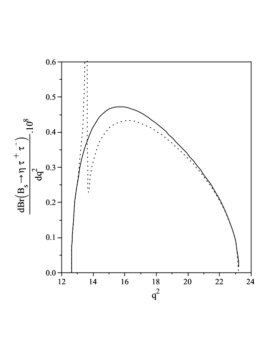
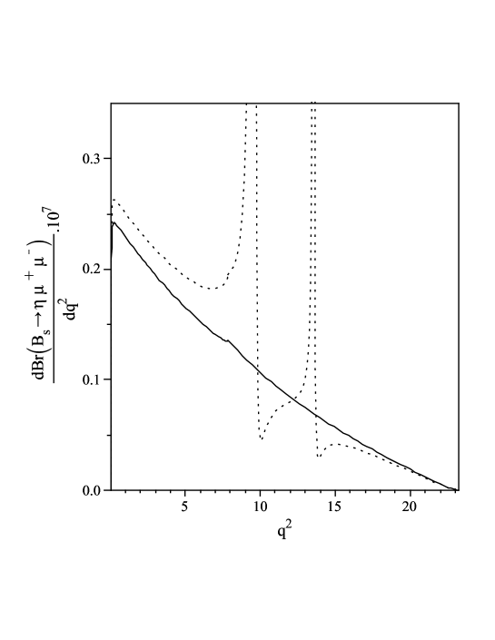
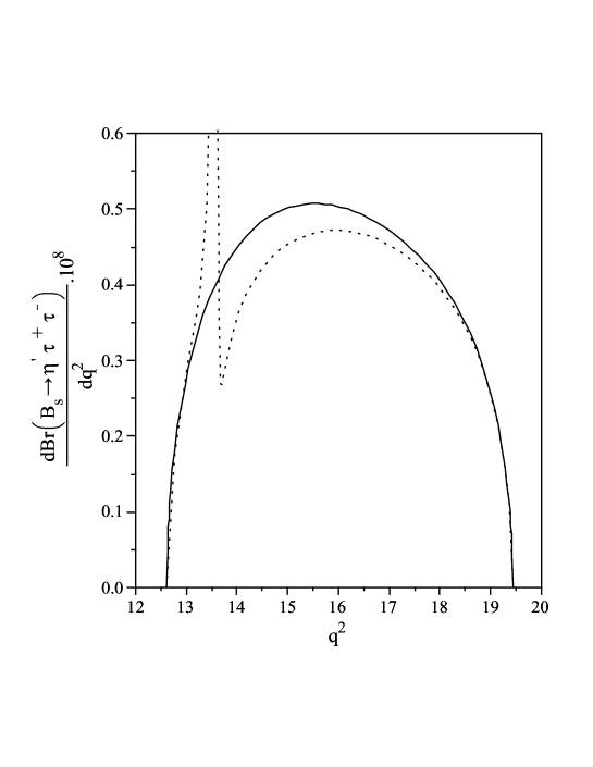
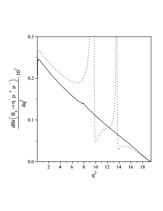
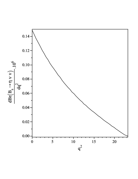
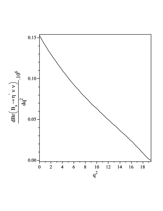
corrections and the corresponding matrix elements may also be sensitive to the isosinglet content of the and mesons. We show the dependency of the differential
branching ratios on (with and without LD effects for
charged lepton case) in Figs. (8)-(13).
Mode
I
II
III
Table 4: The branching ratios of the semileptonic
decays including LD
effects.
Mode
I
II
Table 5: The branching ratios of the semileptonic
decays including LD
effects.
Finally, we want to calculate the longitudinal lepton polarization
asymmetry for considered decays. It is given as Chen :
where and were defined before. The dependence of the
longitudinal lepton polarization asymmetries for the decays on the transferred momentum square
with and without LD effects are plotted in Figs. 14
and 15.
As a result, the order of the obtained values for branching ratios
as well as the longitudinal lepton polarization asymmetries show
a possibility to study the considered transitions at LHC. Any
experimental measurements on the presented quantities and those
comparisons with the obtained results can give valuable
information about the nature of the and mesons and
strong interactions inside them.
Acknowledgments
Partial support of Shiraz university research council is
appreciated.
Appendix–A
In this appendix, the explicit expressions of the
are given,
where, and .
Figure 6: The dependence of the form factors on
at and for . The small
boxes correspond to the values obtained directly from sum rules
and the solid lines belong to the fit parametrization of the form
factors.Figure 7: The dependence of the form factors on
at and for . The
small boxes correspond to the values obtained directly from sum
rules and the solid lines belong to the fit parametrization of
the form factors.
Figure 8: The dependence of the differential
branching fraction of the decay with
and without the LD effects on . The solid and dotted lines
show the results without and with the LD effects,
respectively.
Figure 13: The same as Fig 12 but for the
.Figure 14: The dependence of the Longitudinal lepton
polarization asymmetry on . The left figure belongs to the
decay and the right figure corresponds to
the . The solid lines and dotted lines
show the results without and with the LD effects,
respectively.Figure 15: The same as Fig 14 but for the transition.
References
(1)
M. Artuso et al., (CLEO Collaboration), Phys. Rev. Lett. 95,
261801 (2005).
(2)
G. Bonvicini et al., (CLEO Collaboration), Phys. Rev. Lett. 96,
022002 (2006).
(3)
A. Drutskoy, arXiv:0905.2959 [hep-ex].
(4)
G. Buchalla, G. Hiller, G. Isidori, Phys. Rev. D 63, 014015
(2000).
(5)
C. Bird, P. Jackson, R. Kowalewski, M. Pospelov, Phys. Rev. Lett.
93, 201803 (2004).
(6)
T. Feldmann, P. Kroll, B. Stech, Phys. Rev. D 58, 114006 (1998);
Phys. Lett. B 449, 339 (1999); T. Feldmann, Int. J. Mod. Phys. A
15, 159 (2000).
(7)
F. De Fazio, M. R. Pennington, JHEP 0007, 051 (2000).
(8)
H. M. Choi, J. Phys. G 37, 085005 (2010).
(9)
M. V. Carlucci, P. Colangelo, De. F. Fazio, Phys. Rev. D 80,
055023 (2009).
(10)
F. Ambrosino et al. (KLOE Collaboration), Phys. Lett. B 648, 267
(2007).
(11)
C. Amsler et al., Particle Data Group, Phys. Lett. B 667, 1
(2008).
(12)
A. J. Buras, M. Muenz, Phys. Rev. D 52, 186 (1995).
(13)
J. Rolf, M. Della Morte, S. Durr, J. Heitger, A. Juttner, H.
Molke, A. Shindler, R. Sommer, Nucl. Phys. Proc. Suppl. 129, 322
(2004).
(14)
P. Ball, R. Zwicky, Phys. Rev. D 71, 014015 (2005).
(15)
C. H. Chen, C. Q. Geng, C. C. Lih, C. C. Liu, Phys. Rev. D 75,
074010 (2007).
(16)
C. Q. Geng, C. C. Liu, J. Phys. G 29, 1103 (2003).
(17)
A. Faessler, Th. Gutsche, M. A. Ivanov, J. G. Körner, V. E.
Lyubovitskij, Eur. Phys. J. C 4, 18 (2002).