Trapped two-component Fermi gases with up to six particles: Energetics, structural properties, and molecular condensate fraction

Abstract

We investigate small equal-mass two-component Fermi gases under external spherically symmetric confinement in which atoms with opposite spins interact through a short-range two-body model potential. We employ a non-perturbative microscopic framework, the stochastic variational approach, and determine the system properties as functions of the interspecies $s$-wave scattering length $a_{s}$, the orbital angular momentum $L$ of the system, and the numbers $N_{1}$ and $N_{2}$ of spin-up and spin-down atoms (with $N_{1}-N_{2}=0$ or 1 and $N\leq 6$, where $N=N_{1}+N_{2}$). At unitarity, we determine the energies of the five- and six-particle systems for various ranges $r_{0}$ of the underlying two-body model potential and extrapolate to the zero-range limit. These energies serve as benchmark results that can be used to validate and assess other numerical approaches. We also present structural properties such as the pair distribution function and the radial density. Furthermore, we analyze the one-body and two-body density matrices. A measure for the molecular condensate fraction is proposed and applied. Our calculations show explicitly that the natural orbitals and the momentum distributions of atomic Fermi gases approach those characteristic for a molecular Bose gas if the $s$-wave scattering length $a_{s}$, $a_{s}>0$, is sufficiently small.

I Introduction

Over the past few years, the interest in small trapped Bose and Fermi gases, and mixtures thereof, has increased tremendously for a number of reasons. First, atomic gases provide an ideal platform for investigating phenomena related to Efimov physics efim71 ; efim73 ; braa06 . While the majority of investigations of the Efimov effect have focused on the three-body system, larger systems have attracted considerable attention recently from theoretical and experimental groups plat04 ; yama06 ; hann06 ; hamm07 ; stec09a ; wang09 ; stec10 ; yama10 ; cast10 ; ferl09 ; zacc09 ; poll09 . Second, small trapped atomic systems can be realized by loading an atomic gas into an optical lattice grei02 ; koeh05 ; thal06 ; bloc08 . If the tunneling between lattice sites is small and if the interactions between neighboring sites can be neglected, then each lattice site provides a realization of a trapped few-body system. In this setting, one interesting prediction is that effective three- and higher-body interactions should emerge johnsonNJP . Third, small atomic gases can be viewed as a bridge between two-body and many-body systems (see, e.g., Refs. blum07 ; stec08 ; chan07 ; bulg07 ). In most cases, the two-body system is well characterized, making a bottom-up approach attractive. Such an approach treats increasingly larger systems and eventually connects observables for mesoscopic systems with those predicted by many-body theories, e.g., through the use of the local density approximation. Fourth, few-body systems often times allow for highly accurate treatments, thereby providing much needed benchmark results. For example, a number of lattice-based approaches are presently being applied to trapped cold atom systems (see Refs. chen04 ; bulg06 ; buro06 ; lee06 ; lee06a ; abe09 for lattice-based treatments of the homogeneous system). While these approaches promise to be very powerful, currently only a few benchmark results are available that allow for a careful assessment of their validity regimes.

This paper treats equal-mass two-component Fermi gases under external harmonic confinement with short-range $s$-wave interactions. Our work builds on the rapidly expanding number of papers that treat trapped three-dimensional few-fermion systems (see, e.g., Refs. blum07 ; stec08 ; chan07 ; bulg07 ; cast04 ; wern06 ; wern06a ; kest07 ; stet07 ; stec07c ; stec07b ; alha08 ; blumpolarized ; blum09a ; liu09 ; dail10 ). The ground state of trapped equal-mass two-component Fermi gases, e.g., has been investigated numerically by the fixed-node diffusion Monte Carlo approach blum07 ; stec08 ; chan07 ; blumpolarized and the stochastic variational approach stec07c ; blum07 ; stec08 ; blum09a ; dail10 . In the strongly-interacting unitary regime, the properties of the system—motivated by analytical treatments that exploit the scale invariance of equal-mass Fermi gases at unitarity cast04 ; wern06 —have been interpreted within the hyperspherical framework blum07 ; stec08 . In some cases, the excitation spectrum at unitarity has also been investigated blum07 ; stec08 ; wern06 ; wern06a . In addition, small two-component Fermi gases have been investigated as a function of the $s$-wave scattering length $a_{s}$ kest07 ; stec07c ; stet07 ; stec07b ; stec08 ; liu09 ; blum09a ; dail10 . For small $|a_{s}|$, $a_{s}<0$, the energy crossover curve has been analyzed by applying first order perturbation theory to a weakly-attractive atomic Fermi gas stec07b ; stec08 ; dail10 . For small $|a_{s}|$, $a_{s}>0$, in contrast, the energy crossover curve has been analyzed by applying first order perturbation theory to a weakly-repulsive molecular gas stec07b ; stec08 ; dail10 (see also Refs. astr04c ; petr04aa ; petr05 ). Small two-component Fermi gases have also provided the first high precision tests blum09a of the Tan relations tan08a ; tan08b ; tan08c that apply to both inhomogeneous and homogeneous $s$-wave interacting Fermi gases.

Following up on our earlier work, this paper presents new results for trapped equal-mass Fermi gases with up to $N=6$, where $N=N_{1}+N_{2}$ and $N_{1}-N_{2}=0$ or 1. Our main results are: (i) We report extrapolated zero-range energies for five- and six-particle systems with $(N_{1},N_{2})=(3,2)$ and $(3,3)$ for various angular momenta at unitarity. (ii) We present energy crossover curves for the $(N_{1},N_{2})=(3,2)$ system for the ground state and various excited states. (iii) We present a detailed analysis of the dependence of the few-particle energies on the range of the underlying two-body potential. (iv) We present structural properties for the $(N_{1},N_{2})=(2,1)$, $(2,2)$, $(3,2)$ and $(3,3)$ systems throughout the crossover, including unitarity. (v) We quantify the correlations of few-fermion systems by analyzing the one- and two-body density matrices as well as the momentum distributions. In particular, we propose a measure of the molecular condensate fraction and apply it to few-fermion systems with up to $N=6$ atoms. Related analyses have previously been pursued for bosonic gases dubo01 ; mous02 ; thog07 and one-dimensional systems gira00 ; deur07 ; casu08 , but we are not aware of analogous studies for trapped three-dimensional two-component Fermi gases.

Section II introduces the system Hamiltonian and the stochastic variational approach employed to solve the time-independent Schrödinger equation for small trapped two-component systems. In addition, Sec. II reviews the definitions of the one- and two-body density matrices and their relationship to the natural orbitals and momentum distribution. Section III presents and interprets our results for various parameter combinations. Lastly, Section IV summarizes our main results and concludes. Mathematical derivations and discussions of technical aspects are collected in Appendices A through C.

II Theoretical background

II.1 System Hamiltonian

Our model Hamiltonian that describes equal-mass two-component Fermi gases with $N_{1}$ spin-up and $N_{2}$ spin-down atoms ($N=N_{1}+N_{2}$ and $N_{1}\geq N_{2}$) under external spherically symmetric harmonic confinement with angular trapping frequency $\omega$ reads

$$H=\sum_{j=1}^{N}\left(\frac{-\hbar^{2}}{2m_{a}}\nabla_{\vec{r}_{j}}^{2}+\frac{1}{2}m_{a}\omega^{2}\vec{r}_{j}^{2}\right)+$$

$$\sum_{j=1}^{N_{1}}\sum_{k=N_{1}+1}^{N}V_{\mathrm{tb}}(r_{jk}).$$ (1)

Here, $m_{a}$ denotes the atom mass and $\vec{r}_{j}$ the position vector of the $j$th particle measured with respect to the trap center (with $r_{jk}=|\vec{r}_{j}-\vec{r}_{k}|$); the first $N_{1}$ position vectors correspond to the spin-up atoms and the last $N_{2}$ position vectors to the spin-down atoms. Hamiltonian (II.1) assumes that like fermions are non-interacting. The interspecies interactions are modeled through a purely attractive Gaussian two-body potential $V_{\mathrm{tb}}(r)$,

$$V_{\mathrm{tb}}(r)=-V_{0}\exp\left[-\left(\frac{r}{\sqrt{2}r_{0}}\right)^{2}\right].$$ (2)

We take the range $r_{0}$ to be much smaller than the harmonic oscillator length $a_{\mathrm{ho}}$, where $a_{\mathrm{ho}}=\sqrt{\hbar/(m_{a}\omega)}$. The depth $V_{0}$, $V_{0}>0$, and the range $r_{0}$ are adjusted so that the free-space two-body $s$-wave scattering length $a_{s}$ takes on the desired value. We restrict ourselves to two-body potentials that support no free-space $s$-wave two-body bound state and one free-space $s$-wave two-body bound state for negative $a_{s}$ and positive $a_{s}$, respectively. If the scattering length $a_{s}$ is notably larger than the range $r_{0}$, then the properties of small trapped two-component Fermi gases are universal, i.e., independent of the details of the underlying two-body potential gior08 ; astr04c ; bake99 ; ohar02 ; ho04 ; tan04 ; chan05 ; chan04a ; thom05 ; son06 ; stew06 . Thus, we limit ourselves to parameter combinations with $r_{0}\ll a_{s}$ and $r_{0}\ll a_{\mathrm{ho}}$. For these parameter combinations, energy shifts due to $p$-wave or higher partial wave scattering between unlike fermions are negligible. In a few cases, we perform calculations for different $r_{0}$ and explicitly extrapolate to the $r_{0}\rightarrow 0$ limit.

Our goal is to solve the time-independent Schrödinger equation for the Hamiltonian given in Eq. (II.1), and to analyze the energy spectrum and structural properties. To this end, we use that the total wave function $\psi_{\mathrm{tot}}(\vec{r}_{1},\cdots,\vec{r}_{N})$ separates into a relative part $\psi_{\mathrm{rel}}$ and a center-of-mass part $\psi_{\mathrm{cm}}$. The relative wave function $\psi_{\mathrm{rel}}$ is written in terms of Jacobi vectors $\vec{\rho}_{1},\cdots,\vec{\rho}_{N-1}$; its determination through the stochastic variational approach is reviewed briefly in the next subsection. Throughout, we assume that center-of-mass excitations are absent, i.e., we assume that the center of mass wave function is given by

$$\psi_{\mathrm{cm}}(\vec{R}_{\mathrm{cm}})=N_{\mathrm{cm}}\exp\left(-\frac{\vec{R}_{\mathrm{cm}}^{2}}{2a_{\mathrm{ho}}^{2}/N}\right),$$ (3)

where $N_{\mathrm{cm}}$ denotes a normalization constant and $\vec{R}_{\mathrm{cm}}$ the center of mass vector, $\vec{R}_{\mathrm{cm}}=\sum_{j=1}^{N}\vec{r}_{j}/N$. The relative wave function $\psi_{\mathrm{rel}}$ is a simultaneous eigen function of the relative Hamiltonian $H_{\mathrm{rel}}$, the square of the relative orbital angular momentum operator, the $z$-projection of the relative orbital angular momentum operator and the parity operator. Correspondingly, $\psi_{\mathrm{rel}}$ and the associated eigen energies $E_{\mathrm{rel}}$ are labeled by the quantum numbers $L$, $M_{L}$ and $\Pi$.

II.2 Stochastic variational treatment

To determine the relative eigen functions $\psi_{\mathrm{rel}}$ and relative eigen energies $E_{\mathrm{rel}}$, we employ the stochastic variational (SV) approach varg95 ; varg01 ; cgbook ; sore05 . Our implementation follows that described in Refs. stec07c ; stec08 ; dail10 , and here we only emphasize a few key points. The SV approach expands the relative wave function $\psi_{\mathrm{rel}}$ in terms of a basis set. The basis functions themselves are not linearly independent, and the determination of the eigen energies requires the solution of a generalized eigen value problem that involves the Hamiltonian matrix and the overlap matrix. Just as with other basis set expansion techniques, the SV approach results in a variational upper bound to the exact eigen energies, i.e., to the ground state energy and to the energies of excited states. For the interaction and confining potentials chosen in this work, the functional forms of the basis functions allow for an analytical evaluation of the Hamiltonian and overlap matrix elements. The proper fermionic symmetry of the basis functions is ensured through the application of a permutation operator ${\cal{A}}$. For the $(3,3)$ system, e.g., ${\cal{A}}$ consists of 36 permutations (6 permutations each are required to anti-symmetrize the three spin-up and the three spin-down fermions).

While the functional forms of the basis functions are relatively simple, they are sufficiently flexible to describe short-range correlations that develop on a length scale of the order of the range $r_{0}$ and long-range correlations that develop on a length scale of the order of the oscillator length $a_{\mathrm{ho}}$ stec07c . This is achieved through the use of a comparatively large number of variational parameters that are optimized semi-stochastically for each basis function. In this work, we employ basis functions that are characterized by $N(N-1)/2$ to $N(N-1)/2+3(N-1)$ parameters [see Eq. (19) of Appendix A for an explicit expression for the basis functions with $L^{\Pi}=0^{+}$ symmetry and Eq. (6.27) of Ref. cgbook , or Eqs. (36) and (37) of Ref. dail10 , for an explicit expression of the basis functions with arbitrary $L$ employed in this work]. Generally speaking, the treatment of states with $L^{\Pi}=0^{+}$ is numerically less challenging than that of states with other symmetries. As the range $r_{0}$ decreases or $N$ increases, the numerical complexity of the calculation increases. Also, for a given $r_{0}$ and $(N_{1},N_{2})$ combination, the numerical complexity increases with increasing angular momentum. The largest calculation reported in Sec. III uses $N_{b}=3000$, where $N_{b}$ is the number of fully anti-symmetrized basis functions. In many cases, however, the optimization procedure of the variational parameters is more important than the size of the basis set itself. In our implementation, e.g., a notable fraction of the computational efforts is directed at optimizing the basis functions for a given $N_{b}$ as opposed to increasing $N_{b}$. The motivation for keeping the basis set relatively small is two-fold. First, the use of highly optimized basis functions mitigates essentially all problems that would otherwise arise from the linear dependence of the basis functions stec07c ; cgbook . Second, the computational time required to calculate structural properties increases with increasing $N_{b}$.

To calculate structural properties, we follow two different approaches. Where possible, we determine the matrix elements for a given operator $A$ analytically, and determine the quantity $\langle\psi_{\mathrm{tot}}|A|\psi_{\mathrm{tot}}\rangle/\langle\psi_{\mathrm{tot}}|\psi_{\mathrm{tot}}\rangle$ by simply adding all matrix elements weighted by the appropriate expansion coefficients. This approach scales quadratically with $N_{b}$ and is, in most cases, more efficient than our second approch, a variational Monte Carlo calculation montecarlo that uses the wave function optimized by the stochastic variational approach. In particular, we calculate structural observables by performing a Metropolis walk that samples the probability distribution $|\psi_{\mathrm{tot}}|^{2}/\langle\psi_{\mathrm{tot}}|\psi_{\mathrm{tot}}\rangle$. The expectation value of $A$ is then determined by averaging over many possible realizations of the system. At each step, the density $|\psi_{\mathrm{tot}}|^{2}$ needs to be calculated, resulting in a scaling of the computational effort with $N_{b}N_{\mathrm{sample}}$, where the number of Metropolis steps $N_{\mathrm{sample}}$ is generally much larger than $N_{b}$. Appendix B details the Monte Carlo sampling scheme for a number of observables that quantify the correlations of the system. A distinct advantage of the Metropolis sampling approach is that it allows for the evaluation of “conditional observables” such as the quantity $\bar{\rho}_{\mathrm{red}}(\vec{R}\,^{\prime},\vec{R})$, defined below Eq. (II.3), for which analytical expressions of the matrix elements are not available.

II.3 Density matrices, occupation numbers and momentum distribution

To quantify the correlations of trapped few-fermion systems, we consider the radial and pair distribution functions as well as the one- and two-body density matrices lowd55 ; penr56 ; yang62 ; leggettbook . The density matrices not only lead to a practical route to determine the momentum distributions associated with the spin-up and spin-down atoms, but also serve to quantify the non-local correlations of the system. For example, for trapped single-species Bose gases, an eigen value of the one-body density matrix of the order of 1 signals a large condensate fraction penr56 ; leggettbook ; dubo01 ; footnotenorm . The situation is different for two-component fermions yang62 ; leggettbook . Because of the anti-symmetric many-body wave function, none of the natural orbitals associated with the one-body density matrix can be occupied macroscopically. In fermionic systems, an appreciable condensate fraction only arises if pairs are being formed yang62 ; leggettbook . To quantify the correlations associated with the formation of pairs, one needs to analyze the two-body density matrix. In the following, we first introduce local structural observables and then non-local observables such as the one-body density matrix and the two-body density matrix. The analysis and discussions presented in this paper are partially motivated by analogous studies of small bosonic ⁴He and fermionic ³He droplets lewa88 . While these systems are significantly more dense than the atomic gases considered here, their characterization is based on the same theoretical framework.

Specifically, we calculate the radial density $P_{1}(\vec{r})$ for the spin-up atoms, where $\vec{r}$ denotes the position vector of the spin-up atoms from the center of the trap. The normalization is chosen such that

$$\int P_{1}(\vec{r})d^{3}\vec{r}=1.$$ (4)

Often times, it is more convenient to record the one-dimensional spherically symmetric component $P_{1,\mathrm{sp}}(r)$,

$$P_{1,\mathrm{sp}}(r)=\int P_{1}(\vec{r}\,^{\prime})\frac{\delta(r-r^{\prime})}{4\pi r^{\prime 2}}d^{3}\vec{r}\,^{\prime},$$ (5)

instead. For $L=1$ states, e.g., the radial density $P_{1}(\vec{r})$ is not spherically symmetric, and $P_{1}(\vec{r})$ and $P_{1,\mathrm{sp}}(r)$ are different. For spin-imbalanced systems, i.e., for systems with $N_{1}-N_{2}>0$, the radial densities for the spin-up and spin-down atoms are different. In this case, we also report $P_{2,\mathrm{sp}}(r)$ for the spin-down atoms, which is defined analogously to $P_{1,\mathrm{sp}}(r)$. Similarly, we calculate the pair distribution function $P_{12,\mathrm{sp}}(r)$ for a spin-up atom and a spin-down atom. The normalization is the same as that for the radial densities, i.e., Eq. (4) applies if $P_{1}(\vec{r})$ is replaced by $P_{12}(\vec{r})$.

In the following, we assume that the total wave function $\psi_{\mathrm{tot}}$ is normalized to 1. The one-body density matrix $\rho_{1}(\vec{r}\,^{\prime},\vec{r})$ for the spin-up atoms is then defined through

$$\rho_{1}(\vec{r}\,^{\prime},\vec{r})=\int\cdots\int\psi_{\mathrm{tot}}^{*}(\vec{r}\,^{\prime},\vec{r}_{2},\cdots,\vec{r}_{N})$$

$$\times\psi_{\mathrm{tot}}(\vec{r},\vec{r}_{2},\cdots,\vec{r}_{N})d^{3}\vec{r}_{2}\cdots d^{3}\vec{r}_{N}.$$ (6)

It can be easily checked that the “diagonal element” $\rho_{1}(\vec{r},\vec{r})$ coincides with the radial density $P_{1}(\vec{r})$. The natural orbitals $\chi_{i}(\vec{r})$ can be defined as those functions that diagonalize the one-body density matrix leggettbook ,

$$\rho_{1}(\vec{r}\,^{\prime},\vec{r})=\sum_{i}n_{i}\chi^{*}_{i}(\vec{r}\,^{\prime})\chi_{i}(\vec{r}),$$ (7)

where

$$\int\chi^{*}_{i}(\vec{r})\chi_{j}(\vec{r})d^{3}\vec{r}=\delta_{ij}.$$ (8)

In Eq. (7), the $n_{i}$ denote the occupation numbers, $\sum_{i}n_{i}=1$, and the subscript “$i$” labels the natural orbitals footnoteadded .

In practice, it is in general impossible to record the six-dimensional one-body density matrix $\rho_{1}(\vec{r}\,^{\prime},\vec{r})$. Thus, we define the projections $\rho_{lm}(r^{\prime},r)$,

$$\rho_{lm}(r^{\prime},r)=\frac{1}{4\pi}$$

$$\times\int\int Y_{lm}^{*}(\theta^{\prime},\varphi^{\prime})\rho_{1}(\vec{r}\,^{\prime},\vec{r})Y_{lm}(\theta,\varphi)d^{2}\Omega_{r^{\prime}}d^{2}\Omega_{r},$$ (9)

where $d^{2}\Omega_{r}=\sin\theta d\theta d\varphi$. To determine the occupation numbers and natural orbitals, we write $\chi_{i}(\vec{r})=\chi_{qlm}(\vec{r})=R_{qlm}(r)Y_{lm}(\Omega_{r})$ and determine the radial parts $R_{qlm}(r)$ and the occupation numbers $n_{qlm}$ by diagonalizing the scaled projected density matrizes $4\pi\rho_{lm}(r^{\prime},r)$ for each $lm$. For a given $lm$, $q=0$ labels the natural orbital with the largest occupation, $q=1$ the natural orbital with the second largest occupation, and so on.

The momentum distribution $n_{1}(\vec{k})$ of the spin-up atoms can be defined in terms of the one-body density matrix $\rho_{1}(\vec{r}\,^{\prime},\vec{r})$ leggettbook ,

$$n_{1}(\vec{k})=$$

$$\frac{1}{(2\pi)^{3}}\int\rho_{1}(\vec{r}\,^{\prime},\vec{r})\exp[-i\vec{k}^{T}\,(\vec{r}-\vec{r}\,^{\prime})]d^{3}\vec{r}\,^{\prime}d^{3}\vec{r}.$$ (10)

Using the definition of the natural orbitals $\chi_{i}(\vec{r})$ from Eq. (7), it is shown readily that Eq. (II.3) is equivalent to

$$n_{1}(\vec{k})=\sum_{i}n_{i}|\tilde{\chi}_{i}(\vec{k})|^{2},$$ (11)

where $\tilde{\chi}_{i}(\vec{k})$ denotes the Fourier transform of $\chi_{i}(\vec{r})$,

$$\tilde{\chi}_{i}(\vec{k})=\frac{1}{(2\pi)^{3/2}}\int\exp(-i\vec{k}^{T}\,\vec{r})\chi_{i}(\vec{r})d^{3}\vec{r}.$$ (12)

As in the case of the radial density, it is convenient to define the spherical component $n_{1,\mathrm{sp}}(k)$ of $n_{1}(\vec{k})$ through

$$n_{1,\mathrm{sp}}(k)=\int n_{1}(\vec{k}\,^{\prime})\frac{\delta(k-k^{\prime})}{4\pi k^{\prime 2}}d^{3}\vec{k}\,^{\prime}.$$ (13)

Appendix A determines analytical expressions for the matrix elements for $\rho_{1}(\vec{r}\,^{\prime},\vec{r})$, $\rho_{lm}(\vec{r}\,^{\prime},\vec{r})$ and $n_{1,\mathrm{sp}}(k)$ for the basis functions that we use to describe states with $L^{\Pi}=0^{+}$ symmetry.

In addition to the one-body density matrix, we consider the two-body density matrix $\rho_{12}(\vec{r}_{\uparrow}\,^{\prime},\vec{r}_{\downarrow}\,^{\prime},\vec{r}_{\uparrow},\vec{r}_{\downarrow})$,

$$\rho_{12}(\vec{r}_{\uparrow}\,^{\prime},\vec{r}_{\downarrow}\,^{\prime},\vec{r}_{\uparrow},\vec{r}_{\downarrow})=\int\psi^{*}_{\mathrm{tot}}(\vec{r}_{\uparrow}\,^{\prime},\vec{r}_{2},\cdots,\vec{r}_{\downarrow}\,^{\prime},\vec{r}_{N_{1}+2},\cdots,\vec{r}_{N})$$

$$\times\psi_{\mathrm{tot}}(\vec{r}_{\uparrow},\vec{r}_{2},\cdots,\vec{r}_{\downarrow},\vec{r}_{N_{1}+2},\cdots,\vec{r}_{N})$$

$$d^{3}\vec{r}_{2}\cdots d^{3}\vec{r}_{N_{1}}d^{3}\vec{r}_{N_{1}+2}\cdots d^{3}\vec{r}_{N},$$ (14)

which is obtained by integrating over all coordinates but the position vectors of one of the spin-up fermions and one of the spin-down fermions. The two-body density matrix quantifies the non-local correlations between a spin-up atom and a spin-down atom and thus contains information about the formation of pairs yang62 ; leggettbook . To reduce the dimensionality of $\rho_{12}(\vec{r}_{\uparrow}\,^{\prime},\vec{r}_{\downarrow}\,^{\prime},\vec{r}_{\uparrow},\vec{r}_{\downarrow})$, we introduce the relative coordinate vector $\vec{r}=\vec{r}_{\uparrow}-\vec{r}_{\downarrow}$ and the center-of-mass vector $\vec{R}=(\vec{r}_{\uparrow}+\vec{r}_{\downarrow})/2$ (and analogously for the primed coordinates), and rewrite the two-body density matrix in terms of these new coordinate vectors, i.e., we transform to a new set of coordinates. We then define the reduced two-body density matrix $\rho_{\mathrm{red}}(\vec{R}\,^{\prime},\vec{R})$ through

$$\rho_{\mathrm{red}}(\vec{R}\,^{\prime},\vec{R})=$$

$$\int\rho_{12}\left(\vec{R}\,^{\prime}+\frac{\vec{r}}{2},\vec{R}\,^{\prime}-\frac{\vec{r}}{2},\vec{R}+\frac{\vec{r}}{2},\vec{R}-\frac{\vec{r}}{2}\right)d^{3}\vec{r}.$$ (15)

The quantity $\rho_{\mathrm{red}}(\vec{R}\,^{\prime},\vec{R})$ measures the non-local correlations between spin-up—spin-down pairs that are characterized by the same relative distance vector $\vec{r}$. However, as defined the reduced two-body density matrix $\rho_{\mathrm{red}}(\vec{R}\,^{\prime},\vec{R})$ does not distinguish between “small” and “large” pairs. For sufficiently small $a_{s}$ ($a_{s}>0$), we expect that the system consists of $N_{2}$ point-like pairs and $N_{1}-N_{2}$ unpaired atoms and that the $N_{2}$ pairs form a molecular Bose gas. The $(3,2)$ system, e.g., can be thought of as consisting of two pairs and one fermionic impurity when $a_{s}$ is small ($a_{s}>0$); in this case, the pair fraction should be determined by the non-local correlations of the two composite molecules (as opposed to the non-local correlations of all $N_{1}N_{2}=6$ possible pairs). Thus, we define the quantity $\bar{\rho}_{\mathrm{red}}(\vec{R}\,^{\prime},\vec{R})$, which is obtained from $\rho_{\mathrm{red}}(\vec{R}\,^{\prime},\vec{R})$ by only including those $\vec{R}$-vectors that correspond to the position vectors of one of the smallest $N_{2}$ pairs. In practice, we determine $\bar{\rho}_{\mathrm{red}}(\vec{R}\,^{\prime},\vec{R})$ during the Metropolis walk (see Sec. II.3 and Appendix B). While $\rho_{\mathrm{red}}(\vec{R}\,^{\prime},\vec{R})$ is sampled at each step, $\bar{\rho}_{\mathrm{red}}(\vec{R}\,^{\prime},\vec{R})$ is only sampled if the $\vec{R}$ under consideration belongs to that of one of the $N_{2}$ smallest pairs. We note that a related approach has been employed in the Monte Carlo treatment of one-dimensional spin-imbalanced Fermi gases casu08 .

Just as with the one-body density matrix $\rho_{1}(\vec{r}\,^{\prime},\vec{r})$, the reduced two-body density matrix $\rho_{\mathrm{red}}(\vec{R}\,^{\prime},\vec{R})$ can be decomposed into natural orbitals $\chi_{qlm}(\vec{R})$. We refer to the corresponding occupation numbers as $N_{qlm}$; the capital $N$ is chosen to distinguish the occupation numbers associated with $\rho_{\mathrm{red}}(\vec{R}\,^{\prime},\vec{R})$ from those associated with $\rho_{1}(\vec{r}\,^{\prime},\vec{r})$. In analogy to the formalism outlined above for the one-body density matrix, we define the projections $\rho_{lm}(R^{\prime},R)$ and $\bar{\rho}_{lm}(R^{\prime},R)$ of the reduced two-body density matrix. While the occupation numbers $N_{qlm}$ obtained by diagonalizing the $\rho_{lm}(R^{\prime},R)$ add up, by construction, to 1, those obtained by diagonalizing the $\bar{\rho}_{lm}(R^{\prime},R)$ do not. This is a direct consequence of the “conditional sampling approach”. Appendices B and C provide more details about the Monte Carlo sampling and the behavior of ${\rho}_{lm}(R^{\prime},R)$ and $\bar{\rho}_{lm}(R^{\prime},R)$ in the $a_{s}\rightarrow 0^{+}$ limit.

In analogy to Eq. (II.3), the reduced two-body density matrix can be used to obtain the momentum distribution $n_{\mathrm{red}}(\vec{K})$; here, we use $\vec{K}$ instead of $\vec{k}$ to distinguish the momentum vector associated with the position vector of a pair from that of an atom. Similarly, we define $n_{\mathrm{red},\mathrm{sp}}(K)$.

III Results

This section presents our results for small trapped two-component Fermi gases with equal masses. We first present results for the energies of systems with up to $N=6$ particles (see Sec. III.1) and then discuss selected local structural properties (see Sec. III.2). Lastly, Sec. III.3 discusses our results obtained by analyzing non-local observables.

III.1 Energetics

The energetics of the $(2,1)$ and $(2,2)$ systems have been discussed in detail in the literature. Here, we focus on the $(3,2)$ and $(3,3)$ systems. While the qualitative behavior of these larger systems is similar to that of the three- and four-particle systems, the energy spectra of the larger systems is more complex. The increase of the complexity can be traced back to the increased degeneracies in the limits that $a_{s}\rightarrow 0^{-}$ and $a_{s}\rightarrow 0^{+}$. In the weakly-attractive regime ($a_{s}<0$ and $|a_{s}|/a_{\mathrm{ho}}\ll 1$), the so-called BCS regime, the system behaves like a weakly-attractive atomic Fermi gas (see, e.g., Ref. gior08 ). In the weakly-repulsive regime ($a_{s}>0$ and $a_{s}/a_{\mathrm{ho}}\ll 1$), the so-called BEC regime, the system behaves like a weakly-repulsive molecular Bose gas with $N_{1}-N_{2}$ unpaired “fermionic impurities” (see, e.g., Ref. gior08 ). The degeneracies of the non-interacting atomic Fermi gas and the molecular Bose gas with fermionic impurities can be obtained by extending the hyperspherical framework discussed in Ref. dail10 for the $(2,1)$ and $(2,2)$ systems to larger systems. Furthermore, the lifting of the degeneracies, i.e., the slope of each energy level for small $|a_{s}|$, $a_{s}<0$ and $a_{s}>0$, can be obtained by applying first order degenerate perturbation theory using Fermi’s pseudo-potential stec07b ; stec08 ; dail10 . While these limiting behaviors can be obtained fairly straightforwardly, the behavior of the energy levels in the strongly-correlated regime, i.e., in the regime where $|a_{s}|/a_{\mathrm{ho}}\gtrsim 1$, is, in general, non-trivial. In the following, we highlight selected features of the energy spectra of the $(3,2)$ and $(3,3)$ systems.

Figure 1 shows the energies

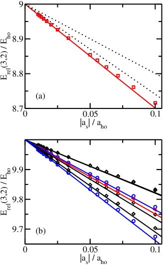
Figure 1: (Color online) Energies $E_{\mathrm{rel}}$ of the $(3,2)$ system in the weakly-attractive regime as a function of $|a_{s}|$, $a_{s}<0$. (a) Energy manifold around $E_{\mathrm{rel,ni}}=9\hbar\omega$. Squares show the SV energies for the state with $1^{-}$ symmetry while a solid line shows the energies obtained within first order degenerate perturbation theory. Dotted lines show the perturbative energies for the unnatural parity states with $0^{-}$ symmetry (upper curve) and $2^{-}$ symmetry (lower curve with 5-fold degeneracy). (b) Energy manifold around $E_{\mathrm{rel,ni}}=10\hbar\omega$. Circles, diamonds and triangles show the SV energies for the states with $0^{+}$ symmetry (two levels with 1-fold degeneracy each), $2^{+}$ symmetry (four levels with 5-fold degeneracy each; the upper two curves are nearly degenerate) and $4^{+}$ symmetry (one level with 9-fold degeneracy), respectively, while solid lines show the energies obtained within first order degenerate perturbation theory. The unnatural parity states with $1^{+}$ and $3^{+}$ symmetry are not shown. The SV calculations are performed for $r_{0}=0.05a_{\mathrm{ho}}$. The harmonic oscillator energy $E_{\mathrm{ho}}$ is defined as $E_{\mathrm{ho}}=\hbar\omega$.

of the $(3,2)$ system in the weakly-attractive regime as a function of $|a_{s}|$ for the first two energy manifolds around the non-interacting energies $E_{\mathrm{rel,ni}}=9\hbar\omega$ and $E_{\mathrm{rel,ni}}=10\hbar\omega$. These energy manifolds consist of a total of 9 and 57 states, respectively (see Table 1).

Table 1: Dimensionless coefficients $c^{(1)}$ that characterize the weakly-attractive Fermi gas for the $(N_{1},N_{2})=(3,2)$ system. The $c^{(1)}$ are defined through $E^{(1)}=c^{(1)}(2\pi)^{-1/2}\hbar\omega a_{s}/a_{\mathrm{ho}}$, where $E^{(1)}$ denotes the first order perturbative energy shift, i.e., $E_{\mathrm{rel}}\approx E_{\mathrm{rel,ni}}+E^{(1)}$. $E_{\mathrm{rel,ni}}$ denotes the relative energy of the non-interacting system and $g_{\mathrm{rel,ni}}$ the degeneracy, i.e., $g_{\mathrm{rel,ni}}=2L+1$.

$E_{\mathrm{rel,ni}}/(\hbar\omega)$	$g_{\mathrm{rel,ni}}$	$L^{\pi}$	$c^{(1)}$
9	5	$2^{-}$	$13/2$
9	3	$1^{-}$	$15/2$
9	1	$0^{-}$	$5$
10	9	$4^{+}$	$25/4$
10	7	$3^{+}$	$21/4$
10	7	$3^{+}$	$9/2$
10	5	$2^{+}$	$7.77155$
10	5	$2^{+}$	$6.65010$
10	5	$2^{+}$	$9/2$
10	5	$2^{+}$	$4.45335$
10	3	$1^{+}$	$\frac{1}{16}(87+\sqrt{209})$
10	3	$1^{+}$	$\frac{1}{16}(87-\sqrt{209})$
10	3	$1^{+}$	$\frac{1}{8}(33+\sqrt{89})$
10	3	$1^{+}$	$\frac{1}{8}(33-\sqrt{89})$
10	1	$0^{+}$	$\frac{5}{16}(23+\sqrt{17})$
10	1	$0^{+}$	$\frac{5}{16}(23-\sqrt{17})$

For comparison, the lowest energy manifold of the $(2,1)$ and $(2,2)$ systems contains only 3 and 9 states, respectively, and the second lowest energy manifold of these systems contains only 9 and 27 states, respectively dail10 . The ground state of the ($3,2)$ system has $L^{\Pi}=1^{-}$ symmetry and is 3-fold degenerate (the degeneracy $g_{\mathrm{rel,ni}}=3$ is due to the spherical symmetry and is associated with the azimuthal quantum number $M_{L}$, $M_{L}=-L,-L+1,\cdots,L$). The two excited states of the lowest energy manifold [dotted lines in Fig. 1(a)] correspond to unnatural parity states with $0^{-}$ and $2^{-}$ symmetry. For $|a_{s}|/a_{\mathrm{ho}}\ll 1$, the perturbative treatment describes the energy spectrum accurately. As expected, the description worsens as $|a_{s}|/a_{\mathrm{ho}}$ increases. We note that the finite-range effects of the SV energies are smaller than the symbol size; consequently, the deviations between the SV energies and the perturbative energies are predominantly due to the approximate nature of the perturbative treatment, which assumes zero-range interactions, and not due to the fact that Fig. 1 compares energies obtained for finite-range and zero-range interactions. The perturbative treatment provides a qualitatively correct picture up to $|a_{s}|/a_{\mathrm{ho}}\approx 0.5$ (note that Fig. 1 only covers the values $|a_{s}|/a_{\mathrm{ho}}\leq 0.1$). Figure 1(b) shows the energy levels corresponding to natural parity states of the first excited state energy manifold of the $(3,2)$ system around $E_{\mathrm{rel,ni}}=10\hbar\omega$. For comparison, Fig. 2 exemplarily illustrates for the $(3,3)$ system that the ground state of spin-balanced systems has $0^{+}$ symmetry.

Figure 2: (Color online) Lowest energy manifold of the $(3,3)$ system in the weakly-attractive regime as a function of $|a_{s}|$, $a_{s}<0$. Circles and diamonds show the SV energies for the natural parity states with $0^{+}$ and $2^{+}$ symmetry, respectively, while solid lines show the energies calculated using first order degenerate perturbation theory. In addition, a dotted line shows the perturbative energy for the unnatural parity state with $1^{+}$ symmetry. The SV calculations are performed for $r_{0}=0.05a_{\mathrm{ho}}$.

Table 2 summarizes the degeneracies and

Table 2: Dimensionless coefficients $c^{(1)}$ for the Fermi gas with $(N_{1},N_{2})=(3,3)$. See the caption of Table 1 for details.

$E_{\mathrm{rel,ni}}/(\hbar\omega)$	$g_{\mathrm{rel,ni}}$	$L^{\pi}$	$c^{(1)}$
23/2	5	$2^{+}$	$19/2$
23/2	3	$1^{+}$	$17/2$
23/2	1	$0^{+}$	$11$
25/2	9	$4^{-}$	$33/4$
25/2	9	$4^{-}$	$31/4$
25/2	7	$3^{-}$	$41/4$
25/2	7	$3^{-}$	$\frac{1}{8}(63+\sqrt{33})$
25/2	7	$3^{-}$	$\frac{1}{8}(63-\sqrt{33})$
25/2	5	$2^{-}$	$73/8$
25/2	5	$2^{-}$	$9.04636$
25/2	5	$2^{-}$	$17/2$
25/2	5	$2^{-}$	$8.11599$
25/2	5	$2^{-}$	$6.71264$
25/2	5	$2^{-}$	$11/2$
25/2	3	$1^{-}$	$\frac{1}{16}(137+\sqrt{609})$
25/2	3	$1^{-}$	$9.34613$
25/2	3	$1^{-}$	$8.58664$
25/2	3	$1^{-}$	$\frac{1}{16}(137-\sqrt{609})$
25/2	3	$1^{-}$	$5.94223$
25/2	1	$0^{-}$	$7$
25/2	1	$0^{-}$	$25/4$

perturbative energy shifts for the two lowest energy manifolds of the $(3,3)$ system.

Figure 3 shows selected energy levels for natural parity states of the $(3,2)$ system as a function of $a_{s}^{-1}$ throughout the crossover. Dotted, solid, dash-dotted, dash-dot-dotted and dashed lines show the lowest energy level of the $L=0$ to 4 states with natural parity. Figure 3(a) shows that the $L=1$ state has the lowest energy when $a_{s}$ is negative [see also Fig. 1(a)].

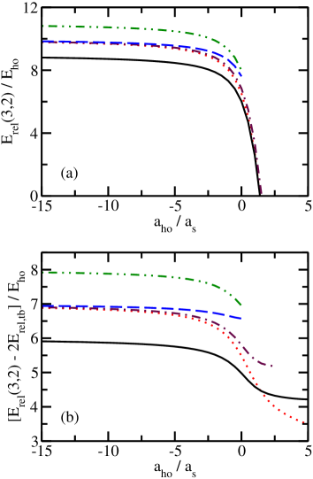
Figure 3: (Color online) SV energies for the natural parity states of the $(3,2)$ system with $r_{0}=0.05a_{\mathrm{ho}}$ as a function of $a_{s}^{-1}$ in the crossover regime. Panel (a) shows the “bare energy” $E_{\mathrm{rel}}$ while panel (b) shows the scaled energy $E_{\mathrm{rel}}-2E_{\mathrm{rel,tb}}$. Dotted, solid, dash-dotted, dash-dot-dotted and dashed lines correspond to the lowest state with $L^{\Pi}=0^{+}$, $1^{-}$, $2^{+}$, $3^{-}$ and $4^{+}$ symmetry, respectively. The $L=2-4$ curves do not extend all the way to $a_{\mathrm{ho}}/a_{s}=10$ since the convergence of the energies on the positive scattering length side becomes more challenging as $L$ increases.

However, when $a_{s}$ is small and positive, the $L=0$ state has lower energy. This can be most clearly seen in Fig. 3(b), which shows the scaled energy $E_{\mathrm{rel}}-2E_{\mathrm{rel,tb}}$, where $E_{\mathrm{rel,tb}}$ denotes the relative ground state energy of two trapped atoms that interact through the same two-body potential as the corresponding five-particle system. The subtraction of the energy of two dimers is motivated by the fact that the fermionic system behaves like a system that consists of $N_{2}$ diatomic molecular bosons and $N_{1}-N_{2}$ fermions astr04c ; stec07b ; stec08 ; kest07 . By subtracting the “internal” two-body binding energy $E_{\mathrm{rel,tb}}$, the energy crossover curves are mapped to a smaller energy interval which more clearly reveals the key physics. For example, a significant fraction of the finite-range effects on the positive scattering length side arises due to the formation of pairs and is removed by subtracting the binding energy of $N_{2}$ dimers. Figure 3(b) shows that the crossing between the $L^{\Pi}=1^{-}$ and $0^{+}$ curves occurs at $a_{\mathrm{ho}}/a_{s}\approx 1.5$ for the $(3,2)$ system. This is slightly larger than the value at which the crossing occurs for the $(2,1)$ system, i.e., $a_{\mathrm{ho}}/a_{s}\approx 1$ kest07 ; stet07 ; stec08 .

We now discuss the infinite scattering length regime, which has received considerable attention for several reasons. On the one hand, this is the regime where the system is most strongly correlated and where no small parameter exists around which to expand. On the other hand, the very same aspect that leads to the strong correlations, namely the infinitely large $s$-wave scattering length, also leads to a scale invariance of the system cast04 ; wern06 . In the zero-range limit, the unitary system is characterized by the same number of length scales as the non-interacting system, which can be shown to imply the separability of the wave function into a hyperradial part and a hyperangular part cast04 ; wern06 . This separability has a number of consequences. One of these is the existence of ladders of energy levels that are separated by $2\hbar\omega$ wern06 ; blum07 . Figure 4 exemplarily illustrates for the $(3,2)$ system with $L^{\Pi}=0^{+}$ symmetry how this $2\hbar\omega$ spacing changes as a function of the range $r_{0}$ of the two-body interaction potential.

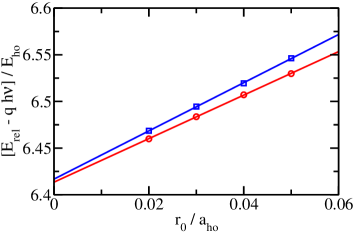
Figure 4: (Color online) Energetics of the $(3,2)$ system with $L^{\Pi}=0^{+}$ at unitarity as a function of $r_{0}$. Circles show the SV energy $E_{\mathrm{rel}}$ ($q=0$ on the $y$-axis label) for the lowest state with $L^{\Pi}=0^{+}$ symmetry, while squares show the shifted SV energy $E_{\mathrm{rel}}-2\hbar\omega$ ($q=1$ on the $y$-axis label) of the second excited state. Solid lines show a linear fit to the SV energies. The intercepts $E_{\mathrm{rel}}(r_{0}=0)$ and slopes are $6.4135(7)\hbar\omega$ and $2.33(2)\hbar\omega/r_{0}$ for the ground state, and $6.417(1)\hbar\omega$ and $2.58(3)\hbar\omega/r_{0}$ for the second excited state, respectively. The numbers in brackets reflect the uncertainty arising from the fit and neglect the basis set extrapolation error of the SV energies.

Circles show the ground state energy while squares show the energy of the second excited state, with $2\hbar\omega$ subtracted, for various $r_{0}$. Figure 4 shows that the finite-range energies approach the zero-range limit linearly from above. The two-paramater fits, shown by solid lines, nearly coincide at $r_{0}=0$, numerically confirming the expected $2\hbar\omega$ spacing with better than $0.1\%$ accuracy. Assuming that a numerically exact treatment gives $E_{\mathrm{rel,gr}}-E_{\mathrm{rel,exc}}=2\hbar\omega$ for $r_{0}=0$, Fig. 4 can be used to assess the accuracy of the SV energies and the extrapolation scheme. Figure 5 shows additional examples for the

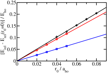
Figure 5: (Color online) Shifted energies $E_{\mathrm{rel}}-E_{\mathrm{rel}}(r_{0}=0)$ at unitarity as a function of $r_{0}$. Circles and squares show the shifted energy of the lowest state of the $(3,2)$ system with $L^{\Pi}=0^{+}$ and $1^{-}$ symmetry, respectively, while diamonds show the shifted energy of the lowest state of the $(3,3)$ system with $L^{\Pi}=0^{+}$. Solid lines show linear fits to the SV energies.

range dependence of the few-body energies at unitarity.

Table 3 summarizes the extrapolated zero-range energies for $N=4-6$.

Table 3: Natural parity zero-range energies $E_{\mathrm{rel}}(N_{1},N_{2})$, in units of $\hbar\omega$, for the two-component equal-mass Fermi gas at unitarity. The energies are obtained by solving a transcendental equation for $N=3$ wern06a . For $N=4,5$ and 6, the energies are obtained by analyzing the SV energies for finite $r_{0}$: The first entry in the third through fifth column is obtained by extrapolating the lowest SV energy for each $r_{0}$ to the $r_{0}\rightarrow 0$ limit (the results for $N=4$ are taken from Ref. dail10 ). The second entry in the third through fifth column is obtained by first extrapolating the SV energies to the $N_{b}\rightarrow\infty$ limit for each $r_{0}$ and by then extrapolating the resulting energies to the $r_{0}\rightarrow 0$ limit.

$L^{\Pi}$	$E_{\mathrm{rel}}(2,1)$	$E_{\mathrm{rel}}(2,2)$	$E_{\mathrm{rel}}(3,2)$	$E_{\mathrm{rel}}(3,3)$
$0^{+}$	3.166	3.509/3.509	6.413/6.395	6.858/6.842
$1^{-}$	2.773	5.598/5.596	5.958/5.955	8.742/8.682
$2^{+}$	4.105	4.418/4.418	6.775/6.774	7.855/7.829
$3^{-}$	4.959	6.176/6.174	7.906/7.898	8.279/8.269
$4^{+}$	6.019	6.485/6.484	7.603/7.601	9.569/9.534
$5^{-}$	6.992	8.245/8.243	8.955/8.945	10.43/10.40
$6^{+}$	8.004	8.496/8.496	9.657/9.653	10.36/10.32

In analyzing our finite range SV energies, we pursued two approaches: The first approach determines the $r_{0}\rightarrow 0$ energies by fitting a linear curve to the lowest SV energies for between 2 and 5 different $r_{0}$ (the results are given by the first entry in the third through fifth column in Table 3). The second approach first extrapolates the SV energies for each $r_{0}$ to the infinite basis set limit, i.e., to the $N_{b}\rightarrow\infty$ limit, and then determines the $r_{0}\rightarrow 0$ energies by fitting the extrapolated SV energies (the results are given by the second entry in the third through fifth column in Table 3). As can be seen, the energies obtained by the second approach lie, as expected, below the energies obtained by the first approach. The second entry in the third through fifth column is our best estimate for the zero-range energy. The errorbars depend on both extrapolations conducted and are not entirely straightforward to determine reliably. For $N=4$ and $L>0$, we estimate the uncertainties to be the larger of $0.005\hbar\omega$ and the absolute value of the difference of the two entries in column three (for $N=4$ and $L=0$, the uncertainty is $0.001\hbar\omega$). For $N=5$ ($N=6$), we estimate the uncertainties to be the larger of $0.01\hbar\omega$ ($0.02\hbar\omega$) and the absolute value of the difference of the two entries in column four (five).

While the range dependence at unitarity varies notably with the symmetry of the system, the energy increases with increasing $r_{0}$ for all systems considered in Table 3. In particular, we find that the slopes vary between about $0.08\hbar\omega/r_{0}$ and about $2.50\hbar\omega/r_{0}$. While the range dependence does, of course, depend on the shape of the two-body potential, we believe that the range dependence for other short-range model potentials is similar to that found here for the Gaussian interaction potential. A more detailed discussion of the dependence of the energies on the range of the two-body potential or the effective range, which characterizes the leading order energy dependence of the two-body $s$-wave phase shift, can be found in Refs. efim93 ; wern08 ; wern10 .

Figure 6 shows the energies of Table 3 graphically.

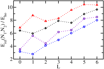
Figure 6: (Color online) Circles, squares, diamonds and triangles show the extrapolated zero-range energy $E_{\mathrm{rel}}(N_{1},N_{2})$ at unitarity as a function of $L$ for the $(2,1)$, $(2,2)$, $(3,2)$, and $(3,3)$ systems, respectively. For each $L$, the energy of the energetically lowest lying natural parity state is shown. Dotted lines are shown to guide the eye. The energies are listed in Table 3.

While we were able to interpret the energies of the $(2,1)$ and $(2,2)$ systems within a simple model (see Ref. dail10 ), we did not find simple analytical expressions that would predict the energies of the $(3,2)$ and $(3,3)$ systems at unitarity with a few percent accuracy. The energies summarized in Table 3 are, to the best of our knowledge, the most extensive and precise esimates of the zero-range energies for systems with $N=5$ and 6, and can be used to assess the accuracy of other numerical approaches. For example, the fixed-node Monte Carlo energies presented in Refs. blum07 ; stec08 for a square well potential with range $0.01a_{\mathrm{ho}}$ are between 0.1% and 4% higher than the zero-range energies reported in the first entry of columns three to five of Table 3. We estimate that roughly up to 1% of the deviations can be attributed to finite-range effects. The remaining discrepancy suggests that the nodal surfaces employed in the fixed-node Monte Carlo calculations are not perfect.

III.2 Local structural properties

This section characterizes local structural properties of small two-component Fermi gases. As discussed in Sec. III.1, the ground state of spin-imbalanced systems with $N_{1}-N_{2}=1$ has $1^{-}$ symmetry in the weakly-attractive regime and $0^{+}$ symmetry in the weakly-repulsive regime, while the ground state of spin-balanced systems has $0^{+}$ symmetry throughout the entire crossover. Motivated by this observation, this section focuses on the energetically lowest lying states with $L^{\Pi}=0^{+}$ and $1^{-}$ symmetry.

Figure 7 shows the pair distribution function $P_{12,\mathrm{sp}}(r)$ for the $(2,1)$ system (dotted lines), the $(2,2)$ system (dashed lines), the $(3,2)$ system (solid lines), and the $(3,3)$ system (dash-dot-dotted lines) with $0^{+}$ symmetry.

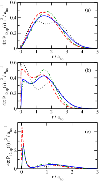
Figure 7: (Color online) Scaled pair distribution function $4\pi\,P_{12,\mathrm{sp}}(r)r^{2}$ for the lowest $L^{\Pi}=0^{+}$ state of the $(2,1)$ system (dotted lines), the $(2,2)$ system (dashed lines), the $(3,2)$ system (solid lines) and the $(3,3)$ system (dash-dot-dotted lines) for (a) $a_{\mathrm{ho}}/a_{s}=-5$, (b) $a_{\mathrm{ho}}/a_{s}=0$ and (c) $a_{\mathrm{ho}}/a_{s}=5$. The calculations for the $(2,1)$ and $(2,2)$ systems are performed using $r_{0}=0.01a_{\mathrm{ho}}$ while those for the $(3,2)$ and $(3,3)$ systems are performed using $r_{0}=0.05a_{\mathrm{ho}}$. The pair distribution functions for the $(2,1)$ and $(2,2)$ systems at unitarity agree with those presented in Ref. stec08 .

Figure 7(a), (b) and (c) show the pair distribution functions for $a_{\mathrm{ho}}/a_{s}=-5$, $0$ and 5, respectively. While the overall behavior of the pair distribution functions for different $N$ but fixed $a_{s}/a_{\mathrm{ho}}$ is similar, small differences exist. For example, for all scattering lengths, the scaled pair distribution functions of the spin-balanced $(2,2)$ and $(3,3)$ systems take on vanishingly small values at smaller $r$ than those of the spin-imbalanced $(2,1)$ and $(3,2)$ systems. This behavior is reversed for the $L^{\Pi}=1^{-}$ states (see Fig. 9). The scaled pair distribution functions $P_{12,\mathrm{sp}}(r)r^{2}$ for $a_{\mathrm{ho}}/a_{s}=-5$ [Fig. 7(a)] have a small but non-vanishing amplitude for $r$ values of the order of $r_{0}$, reflecting the weakly-attractive nature of the two-body interactions. For $a_{\mathrm{ho}}/a_{s}=0$ and $5$, the scaled pair distribution functions $P_{12,\mathrm{sp}}(r)r^{2}$ are characterized by two peaks. As discussed in detail in Ref. stec08 for the $(2,1)$ and $(2,2)$ systems, the two-peak structure arises due to the formation of pairs. While both peaks are broad at unitarity [Fig. 7(b)], the peak at smaller $r$ becomes notably more pronounced as the scattering length becomes positive [Fig. 7(c)]. This can be understood intuitively by realizing that the size of the pairs is, for sufficiently small $a_{s}$ ($a_{s}$ positive), set by $a_{s}$, thereby giving rise to the pronounced peak of $P_{12,\mathrm{sp}}(r)r^{2}$ around $r\approx a_{s}$. The fact that the scaled pair distribution functions go to 0 as $r\rightarrow 0$ is due to the use of finite-range interaction potentials. If we had used zero-range interactions, the amplitude of $P_{12,\mathrm{sp}}(r)r^{2}$ would be finite at $r=0$.

Figure 8 shows the radial densities $P_{1,\mathrm{sp}}(r)$ and $P_{2,\mathrm{sp}}(r)$ for the state with $0^{+}$ symmetry at unitarity for the $(2,1)$ system (dotted lines), the $(2,2)$ system (dashed lines), the $(3,2)$ system (solid lines), and the $(3,3)$ system (dash-dot-dotted lines).

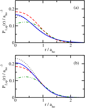
Figure 8: (Color online) Panels (a) and (b) show the radial densities $P_{1,\mathrm{sp}}(r)$ and $P_{2,\mathrm{sp}}(r)$, respectively, for the lowest $L^{\Pi}=0^{+}$ state of the $(2,1)$ system (dotted lines), the $(2,2)$ system (dashed lines), the $(3,2)$ system (solid lines) and the $(3,3)$ system (dash-dot-dotted lines) at unitarity. The calculations for the $(2,1)$ and $(2,2)$ systems are performed using $r_{0}=0.01a_{\mathrm{ho}}$ while those for the $(3,2)$ and $(3,3)$ systems are performed using $r_{0}=0.05a_{\mathrm{ho}}$. The radial density for the $(2,2)$ system agrees with that presented in Ref. stec08 after a proper rescaling (see Ref. footnote1 ).

For the spin-balanced systems, $P_{1,\mathrm{sp}}(r)$ and $P_{2,\mathrm{sp}}(r)$ agree. The peak densities of the $(2,1)$, $(2,2)$ and $(3,2)$ systems are located at $r=0$ while the peak density of the $(3,3)$ system is located at finite $r$. We interpret the fact that the peak density is either located at $r=0$ or at finite $r$ as the system size changes as a signature of (residual) shell structure. Furthermore, Fig. 8(a) shows that the peak density of the majority components of the $(2,1)$ and $(3,2)$ systems is smaller than that of the $(2,2)$ system. The minority components of the spin-imbalanced systems, in contrast, have a higher peak density than the $(2,2)$ system [see Fig. 8(b)]. In interpreting the densities shown in Fig. 8 it is important to keep in mind that the spherical components $P_{1,\mathrm{sp}}(r)$ and $P_{2,\mathrm{sp}}(r)$ are normalized to 1. To “account” for the density of the entire cloud, the densities need to be multiplied by $N_{1}$ and $N_{2}$, respectively.

Figure 9 shows the scaled pair distribution function $P_{12,\mathrm{sp}}(r)r^{2}$ at unitarity for the lowest state with $L^{\Pi}=1^{-}$ symmetry. Qualitatively, the behavior of $P_{12,\mathrm{sp}}(r)r^{2}$ for the lowest states with $L^{\Pi}=1^{-}$ (Fig. 9) and $0^{+}$ [Fig. 7(b)] at unitarity is similar, i.e., $P_{12,\mathrm{sp}}(r)r^{2}$ shows a double-peak structure.

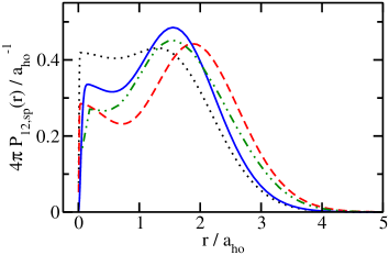
Figure 9: (Color online) Scaled pair distribution function $4\pi\,P_{12,\mathrm{sp}}(r)r^{2}$ for the lowest $L^{\Pi}=1^{-}$ state of the $(2,1)$ system (dotted line), the $(2,2)$ system (dashed line), the $(3,2)$ system (solid line) and the $(3,3)$ system (dash-dot-dotted line) for $a_{\mathrm{ho}}/a_{s}=0$. The calculations for the $(2,1)$ and $(2,2)$ systems are performed using $r_{0}=0.01a_{\mathrm{ho}}$ while those for the $(3,2)$ and $(3,3)$ systems are performed using $r_{0}=0.05a_{\mathrm{ho}}$. The histogram bins of the $(3,3)$ system are wider than those of the other systems, giving rise to the slightly different slope of $P_{12}(r)r^{2}$ at small $r$.

However, as already eluded to, the scaled pair distribution functions for the $L^{\Pi}=1^{-}$ state of the spin-imbalanced systems take on vanishingly small values at smaller $r$ values than those of the spin-balanced systems. For the $(2,1)$ and $(3,2)$ systems, the lowest $L^{\Pi}=1^{-}$ state has a lower energy than the lowest $0^{+}$ state. Thus, a less extended and more compact pair distribution function for the spin-up—spin-down distance is, at least for the systems discussed in Figs. 7 and 9, associated with a lower energy.

III.3 Non-local properties

The pair distribution functions and radial densities discussed in the previous section indicate that small two-component Fermi gases undergo significant changes as the $s$-wave scattering length $a_{s}$ changes from $0^{-}$ over $\infty$ to $0^{+}$. In the $a_{s}\rightarrow 0^{+}$ limit, the basic constituents of the molecular gas are pairs. While the local structural properties provide a great deal of insight into the formation of pairs, they provide no information as to whether or not the pairs are condensed. The determination of the molecular condensate fraction is based, as discussed in Sec. II.3, on the two-body density matrix that measures the “response” of the system to moving a pair from one position in the trap to another position in the trap. The one-body density matrix, in contrast, does not provide a means to quantify the condensate fraction as it measures the response of the system to moving a fermionic atom from one position in the trap to another position in the trap. In the following, we analyze both the one-body and the two-body density matrices.

We first consider non-local properties derived from the one-body density matrix. Figure 10 shows the occupation numbers $n_{qlm}$ [$(qlm)=(000)$, $(100)$ and $(010)$] for the ground state with $L^{\Pi}=0^{+}$ symmetry of the $(2,2)$ system. The behavior is similar for the $(2,1)$, $(3,2)$ and $(3,3)$ systems (not shown). As $a_{s}$ approaches $0^{-}$, the numerically obtained occupation numbers agree with the analytical results presented in Appendix C, i.e., $n_{000}=1/2$, $n_{01m}=1/6$ ($m=0,\pm 1$), and $n_{qlm}=0$ for all other $qlm$. These occupation numbers directly reflect the anti-symmetric character of the non-interacting fermionic system: The two spin-up atoms of the $(2,2)$ system have to occupy different single-particle orbitals. One spin-up atom occupies the lowest harmonic oscillator orbital while the other spin-up atom is equally distributed among the three degenerate first excited state harmonic oscillator orbitals. Figure 10 shows that the occupation numbers $n_{000}$ (solid line) and $n_{010}$ (dotted line) of the $(2,2)$ system change only weakly for $a_{\mathrm{ho}}/a_{s}\lesssim-2.5$, i.e., the one-body density matrix $\rho_{1}(\vec{r}\,^{\prime},\vec{r})$ can be decomposed with fairly good accuracy by including just four natural orbitals.

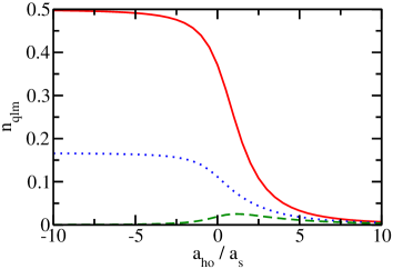
Figure 10: (Color online) Occupation numbers $n_{qlm}$, obtained by analyzing the one-body density matrix $\rho_{1}(\vec{r}\,^{\prime},\vec{r})$, for the lowest state with $0^{+}$ symmetry, i.e., the ground state, of the $(2,2)$ system as a function of the inverse scattering length $a_{s}^{-1}$. Solid, dotted and dashed lines show the occupation numbers $n_{000}$, $n_{010}$ and $n_{100}$, respectively. The occupation numbers $n_{011}$ and $n_{01-1}$ (not shown) are equal to $n_{010}$. The calculations are performed for $r_{0}=0.005a_{\mathrm{ho}}$.

In the strongly-interacting regime, $n_{000}$ and $n_{010}$ decrease notably while other occupation numbers such as $n_{100}$ (dashed line in Fig. 10) increase. In this regime, the system can no longer be thought of as a weakly-perturbed atomic Fermi gas. For $a_{\mathrm{ho}}/a_{s}\gtrsim 5$, we find that a relatively large number of $n_{qlm}$ take on non-vanishing but small values. Intuitively, this can be understood as follows: An expansion of a tight composite boson wave function in terms of effective single particle orbitals (the natural orbitals) requires many terms.

Figures 11 and 12 show results obtained by analyzing the reduced two-body density matrix $\rho_{\mathrm{red}}(\vec{R}\,^{\prime},\vec{R})$. To aid with the interpretation of these results, Fig. 13 compares results obtained by analyzing $\rho_{\mathrm{red}}(\vec{R}\,^{\prime},\vec{R})$ and $\bar{\rho}_{\mathrm{red}}(\vec{R}\,^{\prime},\vec{R})$, respectively; these quantities have been introduced in the last two paragraphs of Sec. II.3 to help quantify the molecular condensate fraction.

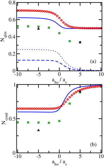
Figure 11: (Color online) Occupation numbers $N_{qlm}$ and condensate fraction $N_{\mathrm{cond}}$, obtained by analyzing the reduced two-body density matrix $\rho_{\mathrm{red}}(\vec{R}\,^{\prime},\vec{R})$, for the energetically lowest-lying state with $0^{+}$ symmetry as a function of the inverse scattering length $a_{s}^{-1}$. (a) Solid, dotted and dashed lines show the occupation numbers $N_{000}$, $N_{100}$, and $N_{010}$, respectively, for the $(2,2)$ system. The occupation numbers $N_{011}$ and $N_{01-1}$ (not shown) are equal to $N_{010}$. For comparison, circles, squares and triangles show the occupation number $N_{000}$ for the $(2,1)$, $(3,2)$ and $(3,3)$ systems, respectively. (b) Circles, the solid line, squares and triangles show the condensate fraction $N_{\mathrm{cond}}$, Eq. (17), for the $(2,1)$, $(2,2)$, $(3,2)$ and $(3,3)$ systems. The calculations are performed for $r_{0}=0.01a_{\mathrm{ho}}$ for the $(2,1)$ system, $r_{0}=0.005a_{\mathrm{ho}}$ for the $(2,2)$ system, and $r_{0}=0.05a_{\mathrm{ho}}$ for the $(3,2)$ and $(3,3)$ systems.

Figure 11(a) shows the occupation numbers $N_{qlm}$ for the lowest state with $0^{+}$ symmetry throughout the crossover for the $(2,1)$, $(2,2)$, $(3,2)$ and $(3,3)$ systems. For the $(2,2)$ system, e.g., $N_{000}$ (solid line) decreases nearly monotonically from $5/8$ in the $a_{s}\rightarrow 0^{-}$ limit to $1/2$ in the $a_{s}\rightarrow 0^{+}$ limit (see Appendix C); in fact, $N_{000}$ reaches a minimum of about $0.495$ at $a_{\mathrm{ho}}/a_{s}\approx 2.5$ and then increases again. While it might be surprising at first sight that the occupation number $N_{000}$ of the lowest natural orbital is larger in the absence of pairs ($a_{s}\rightarrow 0^{-}$ limit) than in the presence of pairs ($a_{s}\rightarrow 0^{+}$ limit), this is a direct consequence of the definition of $\rho_{\mathrm{red}}(\vec{R}\,^{\prime},\vec{R})$: $N_{000}$ is of the order of $1/N_{1}$ in both limits (see Appendix C).

The above discussion indicates that $N_{000}$ does not directly measure the condensate fraction of pairs. Instead, we call the system condensed when the lowest natural orbital is macroscopically occupied, i.e., when $N_{000}$ is much larger than all other $N_{qlm}$, $(qlm)\neq(000)$. Correspondingly, we introduce the quantity $N_{\mathrm{cond}}$,

$$N_{\mathrm{cond}}=1-\frac{\max(\sum_{m=-l}^{l}N_{qlm})}{N_{000}},\;\;(ql)\neq(00).$$ (16)

The summation over $m$ in the second term on the right hand side of Eq. (16) is included since we could have defined the projections [see Eq. (II.3) for the one-body density matrix; the same argument applies to the two-body density matrix] in terms of Legendre polynomials that depend on $l$ only instead of in terms of spherical harmonics that depend on $l$ and $m$. In the $a_{s}\rightarrow 0^{+}$ limit, the second term on the right hand side of Eq. (16) is small and $N_{\mathrm{cond}}$ approaches 1. In the $a_{s}\rightarrow 0^{-}$ limit, the second term on the right hand side of Eq. (16) is of the order of 1 for large numbers of particles and $N_{\mathrm{cond}}$ approaches 0. For small systems, however, $N_{\mathrm{cond}}$ becomes a fraction smaller than 1, i.e., $N_{\mathrm{cond}}=11/17,3/5,0.448,1/3$ for the non-interacting $(2,1)$, $(2,2)$, $(3,2)$ and $(3,3)$ systems, respectively.

In practice, our analysis is limited to a finite number of $(lm)$ projections of the reduced density matrix and Eq. (16) cannot be evaluated as is. Instead, we employ a slightly modified working definition of the condensate fraction $N_{\mathrm{cond}}$,

$$N_{\mathrm{cond}}=1-\frac{\max_{q}(N_{q>0,00},\sum_{m=-1}^{1}N_{q1m})}{N_{000}}.$$ (17)

For the systems studied in this paper, Eqs. (16) and (17) give identical or very similar results. Figure 11(b) illustrates the behavior of $N_{\mathrm{cond}}$, Eq. (17), for the lowest $L^{\Pi}=0^{+}$ state of the $(2,1)$, $(2,2)$, $(3,2)$ and $(3,3)$ systems. Figure 11(b) shows that $N_{\mathrm{cond}}$ increases monotonically from a finite value for $a_{\mathrm{ho}}/a_{s}=-10$ to nearly 1 for $a_{\mathrm{ho}}/a_{s}=10$. Although the quantitative behavior of $N_{\mathrm{cond}}$ depends on the system size, the qualitative behavior is similar for the systems investigated. The condensate fraction $N_{\mathrm{cond}}$ is fairly close to one for $a_{\mathrm{ho}}/a_{s}\gtrsim 5$. The condensate fraction of small few-fermion systems [Fig. 11(b)] exhibits a qualitatively similar behavior to that of the homogeneous system astr05 . The main difference is that $N_{\mathrm{cond}}$ for the trapped system approaches, for the reasons discussed above, a finite value and not a vanishingly small value as $a_{s}\rightarrow 0^{-}$.

To gain further insight into the correlations associated with the pair formation, Fig. 12 exemplarily shows the diagonal element $\rho_{00}(R,R)$, obtained by analyzing the two-body density matrix, for the ground state of the $(2,2)$ system for various scattering lengths.

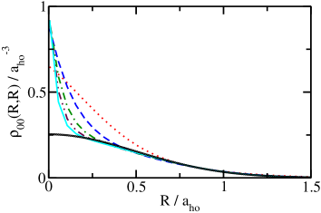
Figure 12: (Color online) Diagonal elements $\rho_{00}(R,R)$, obtained from the reduced two-body density matrix $\rho_{\mathrm{red}}(\vec{R}\,^{\prime},\vec{R})$, for the lowest state with $L^{\Pi}=0^{+}$ symmetry of the $(2,2)$ system for $a_{\mathrm{ho}}/a_{s}=0$ (dotted line), $a_{\mathrm{ho}}/a_{s}=2.5$ (dashed line), $a_{\mathrm{ho}}/a_{s}=5$ (dash-dotted line), $a_{\mathrm{ho}}/a_{s}=7.5$ (dash-dot-dotted line), and $a_{\mathrm{ho}}/a_{s}=10$ [grey (cyan) solid line]. The calculations are performed for $r_{0}=0.005a_{\mathrm{ho}}$. For comparison, the black solid line shows the quantity $\rho_{\mathrm{boson}}(R,R)/2$ [see discussion in the main text and after Eq. (66)].

For small scattering lengths ($a_{s}>0$), i.e., $a_{\mathrm{ho}}/a_{s}\gtrsim 2.5$, the diagonal element $\rho_{00}(R,R)$ contains a broad Gaussian-like background and a sharp shorter-ranged peak. The latter feature becomes narrower with decreasing scattering length. The peak falls off exponentially and is roughly given by the square of the $s$-wave pair function $\Phi_{\mathrm{int}}(r)$, Eq. (68). The sharp peak arises from contributions associated with “large pairs” (see also discussion in the context of Fig. 13). Interestingly, the sharp peak of $\rho_{00}(R^{\prime},R)$ contributes negligibly to the value of $N_{000}$. This can be readily rationalized by realizing that the small $R^{\prime}$ and $R$ parts of $\rho_{00}(R^{\prime},R)$ are highly suppressed due to the radial volume element. The broad Gaussian-like peak is to a fairly good approximation described by $\rho_{\mathrm{boson}}(R,R)/2$ (solid line in Fig. 12). The quantity $\rho_{\mathrm{boson}}(R^{\prime},R)$ is defined in Appendix C after Eq. (66) and denotes the density matrix for a sample of non-interacting molecules of mass $2m_{a}$. In the $a_{s}\rightarrow 0^{+}$ limit, $\rho_{\mathrm{boson}}(R,R)/2$ is expected to provide a good description. The non-diagonal elements [i.e., $\rho_{00}(R^{\prime},R)$ for $R^{\prime}\neq R$, not shown] show qualitatively similar features as the diagonal elements. We find that the broad background of $\rho_{00}(R^{\prime},R)$ approaches $\rho_{\mathrm{boson}}(R^{\prime},R)/2$ as $a_{s}$ approaches the $0^{+}$ limit.

Figure 13 compares the

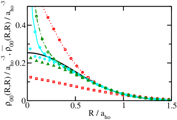
Figure 13: (Color online) Analysis of the reduced two-body density matrix for the lowest state with $0^{+}$ symmetry, i.e., the ground state, of the $(2,2)$ system. Dotted, dash-dotted and grey (cyan) solid lines show the diagonal element $\rho_{00}(R,R)$ obtained by a direct evaluation of the matrix elements for $a_{\mathrm{ho}}/a_{s}=0$, $5$ and $10$, respectively (these data are also shown in Fig. 12). For comparison, circles show $\rho_{00}(R,R)$ for the same scattering lengths but calculated by Monte Carlo sampling; the agreement is excellent. Squares, triangles and diamonds show the diagonal element $\bar{\rho}_{00}(R,R)$ for $a_{\mathrm{ho}}/a_{s}=0$, $5$ and $10$, respectively. The noise visible at small $R$ is a direct consequence of the Monte Carlo sampling aproach. For comparison, the black solid line shows the quantity $\rho_{\mathrm{boson}}(R,R)/2$ [see discussion in the main text and after Eq. (66)].

diagonal elements $\rho_{00}(R,R)$ and $\bar{\rho}_{00}(R,R)$ of the $(2,2)$ system for $a_{\mathrm{ho}}/a_{s}=0$, $5$ and $10$, respectively. The quantity $\bar{\rho}_{00}(R,R)$, determined through Metropolis sampling, accounts only for “large” distances between pairs, thereby reflecting correlations between tightly-bound composite molecules. While the broad peak of $\rho_{00}(R,R)$ nearly coincides with $\bar{\rho}_{00}(R,R)$ for $a_{\mathrm{ho}}/a_{s}=10$, the broad peak of $\rho_{00}(R,R)$ has roughly twice as large of an amplitude as $\bar{\rho}_{00}(R,R)$ for $a_{\mathrm{ho}}/a_{s}=0$. The behavior for the non-diagonal elements, not shown, is similar to that of the diagonal elements. This confirms our interpretation above: The pairs that make up the condensate are those with the smallest interparticle distances. For $a_{\mathrm{ho}}/a_{s}=0$, the $(qlm)=(000)$ orbital is not yet exclusively occupied by the $N_{2}$ smallest pairs but is occupied nearly equally by “small” and “large” pairs. For $a_{\mathrm{ho}}/a_{s}=10$, the $(000)$ orbital is nearly exclusively occupied by large pairs and $\bar{\rho}_{00}(R^{\prime},R)\approx\rho_{\mathrm{boson}}(R^{\prime},R)/2$. This is consistent with our finding above that the condensate fraction is notably smaller than 1 at unitarity. In particular, a value of $N_{000}\approx 1/N_{1}$ at unitary does not signal the condensation of pairs while a value of $N_{000}\approx 1/N_{1}$ in the $a_{s}\rightarrow 0^{+}$ limit, provided all other $N_{qlm}$ are small, does signal the condensation of pairs.

As an alternative to Eq. (16), one could quantify the condensate fraction in terms of the occupation number $\bar{N}_{000}$ associated with $\bar{\rho}_{00}(R^{\prime},R)$, i.e., $\bar{N}_{\mathrm{cond}}=N_{1}\bar{N}_{000}$. While this might be, in certain respects, a more intuitive measure than Eq. (16), the determination of $\bar{\rho}_{00}(R^{\prime},R)$ and thus $\bar{N}_{000}$ is, within our framework, computationally significantly more involved than that of ${\rho}_{00}(R^{\prime},R)$. Thus, we did not apply this alternative measure.

Lastly, we consider the momentum distribution $n_{\mathrm{red},\mathrm{sp}}(K)$ associated with the center-of-mass vector of spin-up—spin-down pairs. Figure 14

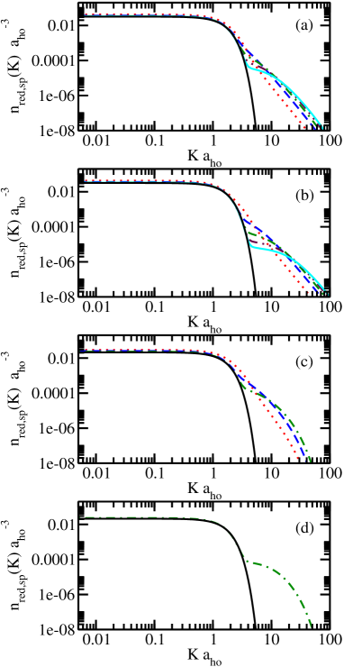
Figure 14: (Color online) Momentum distribution $n_{\mathrm{red},\mathrm{sp}}(K)$ for the lowest state with $L^{\Pi}=0^{+}$ symmetry for (a) the $(2,1)$ system, (b) the $(2,2)$ system, (c) the $(3,2)$ system, and (d) the $(3,3)$ system. Dotted, dashed, dash-dotted, dash-dot-dotted and grey (cyan) solid lines are for $a_{\mathrm{ho}}/a_{s}=0$, $2.5$, $5$, $7.5$ and $10$, respectively (for $N=5$, the largest $a_{\mathrm{ho}}/a_{s}$ considered is $5$; for $N=6$, results are shown for $a_{\mathrm{ho}}/a_{s}=5$ only). For comparison, the dark solid lines show the quantity $n_{\mathrm{boson},\mathrm{sp}}(K)/N_{1}$, Eq. (C) [or first term on the right hand side of Eq. (III.3)]. The calculations for the $(2,1)$, $(2,2)$, $(3,2)$ and $(3,3)$ systems are performed using $r_{0}=0.01a_{\mathrm{ho}}$, $r_{0}=0.005a_{\mathrm{ho}}$, $r_{0}=0.05a_{\mathrm{ho}}$ and $r_{0}=0.05a_{\mathrm{ho}}$, respectively. Note the log-log scale.

shows that $n_{\mathrm{red},\mathrm{sp}}(K)$ consists of two parts, a feature at smaller $K$ ($K\lesssim 5a_{\mathrm{ho}}^{-1}$) and a feature that extends to much larger $K$ values. The emergence of these two features with decreasing $a_{s}$ is another indication of the condensation of pairs. The small and large $K$ features become more distinctly separated as $a_{s}$ decreases. This is in agreement with the increase of $N_{\mathrm{cond}}$ with decreasing $a_{s}$. In fact, Fig. 14 suggests that the few-fermion system can be called condensed when the momentum distribution $n_{\mathrm{red},\mathrm{sp}}(K)$ shows two clearly distinguishable features, i.e., when the derivative of $n_{\mathrm{red},\mathrm{sp}}(K)$ exhibits a significant change for a small change in $K$.

In the $a_{s}\rightarrow 0^{+}$ limit, the momentum distribution $n_{\mathrm{red,sp}}(K)$ for systems with $N_{1}=N_{2}$ is well described by the analytical expression (see Appendix C)

$$n_{\mathrm{red,sp}}(K)\approx\frac{1}{N_{1}}\frac{a_{\mathrm{ho}}^{3}}{{(2\pi)}^{3/2}}\exp\left(-(a_{\mathrm{ho}}{K})^{2}/2\right)+$$

$$\frac{N_{1}-1}{N_{1}}\frac{a_{\mathrm{ho}}^{3}}{\pi^{3/2}Ka_{\mathrm{ho}}}\Re\left[-iA\exp(A^{2})\mathrm{Erfc}(A)\right],$$ (18)

where $A=2a_{\mathrm{ho}}/a_{s}+iKa_{\mathrm{ho}}$ and $\Re$ and $\mathrm{Erfc}$ denote the real part and the complementary error function, respectively. The first term on the right hand side of Eq. (III.3) accounts for the small $K$ feature of $n_{\mathrm{red,sp}}(K)$ and represents the momentum distribution $n_{\mathrm{boson},\mathrm{sp}}(K)/N_{1}$, Eq. (C), derived for non-interacting composite bosons of mass $2m_{a}$ (dark solid lines in Fig. 14). The second term on the right hand side of Eq. (III.3) accounts for the large $K$ feature of $n_{\mathrm{red,sp}}(K)$ and is associated with the internal structure of the composite bosons. In the large $K$ limit, the second term behaves, as expected, as $1/K^{4}$ tan08a ; tan08b ; tan08c . The dependence of the large $K$ part of the momentum distribution on the $s$-wave scattering length $a_{s}$ for systems with $N_{1}=N_{2}$ is reproduced quite accurately by Eq. (III.3). This is illustrated exemplarily for the ground state of the $(2,2)$ system in Fig. 15,

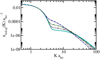
Figure 15: (Color online) Momentum distribution $n_{\mathrm{red},\mathrm{sp}}(K)$ for the lowest state with $L^{\Pi}=0^{+}$ symmetry of the $(2,2)$ system. Dashed, dash-dotted, dash-dot-dotted and grey (cyan) solid lines are for $a_{\mathrm{ho}}/a_{s}=2.5$, $5$, $7.5$ and $10$, respectively [these data are also shown in Fig. 14(b)]. For comparison, the thin solid lines show the analytically predicted momentum distribution $n_{\mathrm{red,sp}}(K)$, Eq. (III.3). Note the log-log scale.

which compares the momentum distribution given by Eq. (III.3) (thin solid lines) with the numerically determined $n_{\mathrm{red,sp}}(K)$ for $a_{ho}/a_{s}=2.5-10$ [same data as shown in Fig. 14(b)]. For $K\gtrsim r_{0}^{-1}$ (not shown in Fig. 15), the momentum distribution given in Eq. (III.3) deviates from that obtained numerically for finite-range interactions. This is expected, since this is the regime where the details of the two-body interaction potential become relevant. The analytical expression for $n_{\mathrm{red,sp}}(K)$ for systems with $N_{1}-N_{2}=1$ and $a_{s}\rightarrow 0^{+}$ differs from Eq. (III.3) and is given in Appendix C, Eq. (C).

IV Conclusions

This paper considers small two-component Fermi gases under external spherically symmetric confinement. We have treated systems with up to $N=6$ atoms, where $N_{1}-N_{2}=0$ or 1, within a microscopic, non-perturbative zero-temperature framework. Using the stochastic variational approach, we have investigated the energetics and structural properties as functions of the $s$-wave scattering length $a_{s}$ and the symmetry of the system. In certain cases, we have also examined the dependence of the results on the range $r_{0}$ of the underlying two-body model potential.

Our analysis of the energetics and the structural properties extends previous studies and adds to the rapidly growing body of results for small trapped three-dimensional few-fermion systems. In particular, we have presented extrapolated zero-range energies for the natural parity states of the five- and six-particle systems at unitarity for various angular momenta. These energies are expected to serve as benchmarks for other numerical approaches.

We have also presented a detailed study of the non-local properties of few-fermion systems. One of our goals has been to quantify the molecular condensate fraction of trapped two-component Fermi systems on the positive scattering length side. To this end, we have analyzed the one-body and the two-body density matrices and proposed to use the quantity $N_{\mathrm{cond}}$ as a measure of the molecular condensate fraction. We showed that the momentum distribution $n_{\mathrm{red,sp}}(K)$, an experimentally accessible observable, develops two clearly distinguishable features at $s$-wave scattering lengths $a_{s}$ for which the molecular condensate fraction $N_{\mathrm{cond}}$ takes on values close to $1$.

The determination of the molecular condensate fraction of the trapped system is more complicated than that of the homogeneous Fermi system since the trap “cuts off” the asymptotic behavior that is typically analyzed to determine the molecular condensate fraction of the homogeneous system (see, e.g., Ref. astr05 for a cold-atom study). Instead, the analysis of finite-sized systems proceeds through the diagonalization of the two-body density matrix. The diagonalization results in a set of natural orbitals and occupation numbers that can then be used to quantify the molecular condensate fraction. In our approach, we measured the position vectors of the composite pairs with respect to the trap center. Alternatively, one might imagine measuring the position vectors with respect to the center of mass of the trapped system. In the context of bosonic systems, implications of defining the one-body density matrix in terms of different “reference coordinates” have been discussed in the literature peth00 ; thog07 ; yama08 ; yama09 . Future work needs to address how the results obtained by analyzing the two-body density matrix of fermionic few-body systems depend on the use of different reference coordinates.

Appendix A Matrix elements employed in stochastic variational approach

While explicit expressions for the Hamiltonian and overlap matrix elements are available in the literature cgbook , explicit expressions for the non-local observables that we are interested in are not. Thus, this appendix outlines the derivation of selected matrix elements used in our SV calculations; our derivations follow the general approach outlined in Ref. cgbook .

In our implementation, we construct the basis set by treating the relative Jacobi vectors $\vec{\rho}_{1},\cdots,\vec{\rho}_{N-1}$ only. The structural properties, however, are determined by multiplying the optimized basis set by the unnormalized ground state center-of-mass wave function $\psi_{\mathrm{cm}}(\vec{R}_{\mathrm{cm}})$ [Eq. (3) with $N_{\mathrm{cm}}=1$]. The unsymmetrized (and unnormalized) basis functions $\phi_{A}$ that include the center-of-mass degrees of freedom and describe states with $L^{\Pi}=0^{+}$ symmetry read

$$\phi_{A}(\vec{x})=\exp\left(-\frac{1}{2}\vec{x}^{T}\,\underline{A}\,\vec{x}\right),$$ (19)

where $\vec{x}$ collectively denotes the $N$ Jacobi vectors, $\vec{x}=(\vec{\rho}_{1},\cdots,\vec{\rho}_{N-1},\vec{R}_{\mathrm{cm}})$. Here, $\underline{A}$ is a symmetric and positive definite matrix that is written in terms of $(N-1)(N-2)/2$ variational parameters [the $(\underline{A})_{jk}$ with $j=1,\cdots,N-1$ and $k\geq j$ are optimized semi-stochastically]. To ensure that the center-of-mass degrees of freedom are in the ground state, the matrix elements $(\underline{A})_{jN}$ and $(\underline{A})_{Nj}$, where $j=1,\cdots,N-1$ are set to zero and the matrix element $(\underline{A})_{NN}$ is set to $N/a_{\mathrm{ho}}^{2}$. The Jacobi vectors $\vec{x}$ and the single particle coordinates $\vec{y}=(\vec{r}_{1},\cdots,\vec{r}_{N})$ are related through the $N\times N$ matrix $\underline{U}$,

$$\vec{x}=\underline{U}\,\vec{y}.$$ (20)

Our first goal is to determine the matrix element $(\rho_{1}(\vec{r}\,^{\prime},\vec{r}))_{A^{\prime}A}=\langle\phi_{A^{\prime}}|\rho_{1}|\phi_{A}\rangle/\langle\phi_{A^{\prime}}|\phi_{A}\rangle$,

$$(\rho_{1}(\vec{r}\,^{\prime},\vec{r}))_{A^{\prime}A}=(O_{A^{\prime}A})^{-1}$$

$$\times\int\left[\int\delta(\vec{r}\,^{\prime}-\vec{r}_{1})\phi_{A^{\prime}}(\vec{x})d^{3}\vec{r}_{1}\right]$$

$$\times\left[\int\delta(\vec{r}-\vec{r}_{1})\phi_{A}(\vec{x})d^{3}\vec{r}_{1}\right]d^{3N-3}\vec{y}_{\mathrm{red}},$$ (21)

where $\vec{y}_{\mathrm{red}}=(\vec{r}_{2},\cdots,\vec{r}_{N})$ and

$$O_{A^{\prime}A}=\left(\frac{(2\pi)^{N}}{\det(\underline{A}^{\prime}+\underline{A})}\right)^{3/2}.$$ (22)

It is convenient cgbook to rewrite the right hand side of Eq. (A) in terms of the function $g(\vec{s};\underline{A},\vec{x})$,

$$g(\vec{s};\underline{A},\vec{x})=\exp\left(-\frac{1}{2}\vec{x}^{T}\,\underline{A}\,\vec{x}+\vec{s}^{T}\vec{x}\right),$$ (23)

where $\vec{s}$ denotes a vector that has the same dimensionality as $\vec{x}$. The unsymmetrized basis functions can then be written as $\phi_{A}(\vec{x})=g(0;\underline{A},\vec{x})$. Using that $\vec{x}^{T}\,\underline{A}\,\vec{x}=\vec{y}^{T}\,\underline{U}^{T}\,\underline{A}\,\underline{U}\,\vec{y}$, we rewrite the unsymmetrized basis functions $\phi_{A}$ in terms of $\vec{y}$ and separate off the $\vec{r}_{1}$ dependence,

$$\phi_{A}(\vec{y})=g(0;\underline{B},\vec{y}_{\mathrm{red}})\exp\left(-\frac{1}{2}b_{1}\vec{r}_{1}^{2}-(\vec{b}^{T}\vec{y}_{\mathrm{red}})^{T}\vec{r}_{1}\right).$$ (24)

Here, the scalar $b_{1}$ is given by $(\underline{U}^{T}\,\underline{A}\,\underline{U})_{11}$, the $(N-1)$-dimensional vector $\vec{b}$ is given by $((\underline{U}^{T}\,\underline{A}\,\underline{U})_{12},\cdots,(\underline{U}^{T}\,\underline{A}\,\underline{U})_{1N})$, and the $(N-1)\times(N-1)$-dimensional matrix $\underline{B}$ is given by $\underline{U}^{T}\,\underline{A}\,\underline{U}$ with the first row and column removed. In Eq. (24), the quantity $(\vec{b}^{T}\vec{y}_{\mathrm{red}})^{T}\vec{r}_{1}$ equals $\sum_{j=2}^{N}(\vec{b})_{j-1}\vec{y}_{j}^{T}\,\vec{r}_{1}$, where $(\vec{b})_{j}$ denotes the $j$th element of the vector $\vec{b}$. To evaluate the right hand side of Eq. (A), we define $b_{1}^{\prime}$, $\vec{b}\,^{\prime}$ and $\underline{B}^{\prime}$ analogously to $b_{1}$, $\vec{b}$ and $\underline{B}$. This yields

$$(\rho_{1}(\vec{r}\,^{\prime},\vec{r}))_{A^{\prime}A}=(O_{A^{\prime}A})^{-1}\int g(0;\underline{B}^{\prime},\vec{y}_{\mathrm{red}})g(0;\underline{B},\vec{y}_{\mathrm{red}})$$

$$\times\exp\left(-\frac{1}{2}b_{1}^{\prime}\vec{r}\,^{\prime 2}-(\vec{b}\,^{\prime}\,{}^{T}\vec{y}_{\mathrm{red}})^{T}\vec{r}\,^{\prime}\right)$$

$$\times\exp\left(-\frac{1}{2}b_{1}\vec{r}^{2}-(\vec{b}^{T}\vec{y}_{\mathrm{red}})^{T}\vec{r}\right)d^{3N-3}\vec{y}_{\mathrm{red}},$$ (25)

which can be rewritten as

$$(\rho_{1}(\vec{r}\,^{\prime},\vec{r}))_{A^{\prime}A}=(O_{A^{\prime}A})^{-1}\int\exp\left(-\frac{1}{2}(b_{1}^{\prime}\vec{r}\,^{\prime}\,{}^{2}+b_{1}\vec{r}^{2})\right)$$

$$g(-(\vec{b}\,^{\prime}\vec{r}\,^{\prime}+\vec{b}\vec{r});\underline{B}^{\prime}+\underline{B},\vec{y}_{\mathrm{red}})d^{3N-3}\vec{y}_{\mathrm{red}}.$$ (26)

Here, the quantity $\vec{b}\vec{r}$ is a $(N-1)$-dimensional vector with elements $(\vec{b})_{j}\vec{r}$, where $j=1,\cdots,N-1$. Using the first entry of Table 7.1 of Ref. cgbook ,

$$\int g(\vec{s};\underline{A},\vec{x})d^{3N}\vec{x}=\left(\frac{(2\pi)^{N}}{\det{\underline{A}}}\right)^{3/2}\exp\left(\frac{1}{2}\vec{s}^{T}\,\underline{A}^{-1}\,\vec{s}\right),$$ (27)

we find a compact expression for the matrix elements of the one-body density matrix,

$$(\rho_{1}(\vec{r}\,^{\prime},\vec{r}))_{A^{\prime}A}=$$

$$(O_{A^{\prime}A})^{-1}c_{1}\exp\left(-\frac{c^{\prime}}{2}\vec{r}\,^{\prime}\,{}^{2}-\frac{c}{2}\vec{r}^{2}+\frac{a}{2}\vec{r}\,^{\prime}\,{}^{T}\vec{r}\right),$$ (28)

where

$$c_{1}=\left(\frac{(2\pi)^{N-1}}{\mathrm{det}(\underline{B}^{\prime}+\underline{B})}\right)^{3/2},$$ (29)

$$c^{\prime}=b_{1}^{\prime}-\vec{b}\,^{\prime}\,{}^{T}\,\underline{C}\,\vec{b}\,^{\prime},$$ (30)

$$c=b_{1}-\vec{b}^{T}\,\underline{C}\,\vec{b},$$ (31)

$$a=\vec{b}\,^{\prime}\,{}^{T}\,\underline{C}\,\vec{b}+\vec{b}^{T}\,\underline{C}\,\vec{b}\,^{\prime},$$ (32)

and

$$\underline{C}=(\underline{B}^{\prime}+\underline{B})^{-1}.$$ (33)

We now use Eq. (A) to determine an analytical expresssion for the matrix element $(\rho_{00}(r^{\prime},r))_{A^{\prime}A}$. To this end, we write $\vec{r}\,^{\prime}\,{}^{T}\vec{r}=r^{\prime}r\cos\gamma$, where $\gamma$ denotes the angle between $\vec{r}\,^{\prime}$ and $\vec{r}$. The integration over $\theta$, $\varphi$, $\theta^{\prime}$ and $\varphi^{\prime}$ then reduces to a single integration over $\gamma$ (the other integrations give a factor of $8\pi^{2}$). Performing the integration over $\gamma$ yields

$$(\rho_{00}({r}^{\prime},{r}))_{A^{\prime}A}=$$

$$(O_{A^{\prime}A})^{-1}\frac{2c_{1}}{ar^{\prime}r}\exp\left[-\frac{1}{2}(c^{\prime}r^{\prime 2}+cr^{2})\right]\sinh\left(\frac{arr^{\prime}}{2}\right).$$ (34)

The matrix elements for higher partial wave projections can be determined in a similar manner.

Our next goal is to determine an analytical expression for the matrix element $(n_{1,\mathrm{sp}}({k}))_{A^{\prime}A}$. Using Eqs. (II.3) and (A), we write

$$(n_{1}(\vec{k}))_{A^{\prime}A}=(O_{A^{\prime}A})^{-1}$$

$$\times\frac{c_{1}}{(2\pi)^{3}}\int\exp\left[-\frac{1}{2}(c^{\prime}r^{\prime 2}+cr^{2}-a\vec{r}\,^{\prime}\,{}^{T}\vec{r})\right]$$

$$\times\exp[i\vec{k}^{T}(\vec{r}\,^{\prime}-\vec{r})]d^{3}\vec{r}\,^{\prime}d^{3}\vec{r}.$$ (35)

Defining $\vec{X}=\vec{r}\,^{\prime}-\vec{r}$, Eq. (A) becomes

$$(n_{1}(\vec{k}))_{A^{\prime}A}=(O_{A^{\prime}A})^{-1}$$

$$\times\frac{c_{1}}{(2\pi)^{3}}\int\exp\left(-\frac{f}{2}r^{2}-\frac{c^{\prime}}{2}X^{2}+\frac{g}{2}\vec{X}^{T}\vec{r}\right)$$

$$\times\exp(i\vec{k}^{T}\vec{X})d^{3}\vec{r}d^{3}\vec{X},$$ (36)

where $f=c^{\prime}+c-a$ and $g=a-2c^{\prime}$. Next, we expand the quantity $\exp(i\vec{k}^{T}\vec{X})$,

$$\exp(i\vec{k}^{T}\vec{X})=\sum_{l=0}^{\infty}(2l+1)i^{l}j_{l}(kX)P_{l}(\cos\gamma^{\prime}),$$ (37)

where $\gamma^{\prime}$ denotes the angle between $\vec{k}$ and $\vec{X}$. Considering the $l=0$ component only, we find

$$(n_{1,\mathrm{sp}}({k}))_{A^{\prime}A}=(O_{A^{\prime}A})^{-1}\frac{c_{1}}{\pi}$$

$$\int_{0}^{\infty}\int_{0}^{\infty}\int_{-1}^{1}\exp\left(-\frac{f}{2}r^{2}-\frac{c^{\prime}}{2}X^{2}+\frac{g}{2}Xr\cos\gamma\right)$$

$$\frac{\sin(kX)}{kX}r^{2}X^{2}d\cos\gamma drdX,$$ (38)

where $\gamma$ denotes the angle between $\vec{r}$ and $\vec{X}$. The integration over $\cos\gamma$ gives

$$(n_{1,\mathrm{sp}}({k}))_{A^{\prime}A}=(O_{A^{\prime}A})^{-1}$$

$$\times\frac{4c_{1}}{\pi gk}\int_{0}^{\infty}\int_{0}^{\infty}\exp\left(-\frac{f}{2}r^{2}-\frac{c^{\prime}}{2}X^{2}\right)$$

$$\sinh\left(\frac{grX}{2}\right)\sin(kX)rdrdX.$$ (39)

If $f>0$, the integration over $r$ can also be performed analytically,

$$(n_{1,\mathrm{sp}}({k}))_{A^{\prime}A}=$$

$$(O_{A^{\prime}A})^{-1}\frac{\sqrt{2}c_{1}}{\sqrt{\pi}f^{3/2}k}\int_{0}^{\infty}\exp\left(-\frac{d}{2}X^{2}\right)\sin(kX)XdX,$$ (40)

where $d$ is given by

$$d=c^{\prime}-\frac{g^{2}}{4f}.$$ (41)

Lastly, the integration over $X$ gives for $d>0$,

$$(n_{1,\mathrm{sp}}({k}))_{A^{\prime}A}=(O_{A^{\prime}A})^{-1}\frac{c_{1}}{(df)^{3/2}}\exp\left(-\frac{k^{2}}{2d}\right).$$ (42)

We have checked numerically that $f$ and $d$ are, indeed, greater than 0.

With one minor change, the derivation outlined above for the matrix elements of the one-body density matrix $\rho_{1}(\vec{r}\,^{\prime},\vec{r})$ also applies to the matrix elements of the reduced two-body density matrix $\rho_{\mathrm{red}}(\vec{R}\,^{\prime},\vec{R})$. In particular, the single-particle coordinate vector $\vec{y}$ needs to be replaced by $(\vec{R},\vec{r},\vec{r}_{2},\cdots,\vec{r}_{N_{1}},\vec{r}_{N_{1}+2},\cdots,\vec{r}_{N})$ and the matrix $\underline{U}$ needs to be redefined accordingly. The derivation of the matrix elements for the quantities $\rho_{00}(R^{\prime},R)$ and $n_{\mathrm{red},\mathrm{sp}}(K)$ then carries over without additional changes.

Appendix B Monte Carlo sampling of density matrix and momentum distribution

This appendix discusses the determination of various observables through the Monte Carlo sampling of the wave function $\psi_{\mathrm{tot}}$. Although our approach follows standard procedures montecarlo ; lewa88 ; dubo01 , we find it useful to summarize a few key results in this appendix for completeness.

Throughout this appendix, we assume that $\psi_{\mathrm{tot}}$ is known but not necessarily normalized. We use a Metropolis walk to generate a set of configurations $(\vec{r}_{1,j},\cdots,\vec{r}_{N,j})$, where $j=1,\cdots,N_{\mathrm{sample}}$, that are distributed according to the probability distribution $P(\vec{r}_{1},\cdots,\vec{r}_{N})$,

$$P(\vec{r}_{1},\cdots,\vec{r}_{N})=$$

$$\frac{|\psi_{\mathrm{tot}}(\vec{r}_{1},\cdots,\vec{r}_{N})|^{2}}{\int|\psi_{\mathrm{tot}}(\vec{r}_{1},\cdots,\vec{r}_{N})|^{2}d^{3}\vec{r}_{1}\cdots d^{3}\vec{r}_{N}}.$$ (43)

Quite generally, the strategy is to express the expectation value of the observable $A$ in terms of $P(\vec{r}_{1},\cdots,\vec{r}_{N})$ and an “auxiliary function” $A^{\prime}$,

$$\langle A\rangle=\int P(\vec{r}_{1},\cdots,\vec{r}_{N})A^{\prime}(\vec{r}_{1},\cdots,\vec{r}_{N})d^{3}\vec{r}_{1}\cdots d^{3}\vec{r}_{N},$$ (44)

and to then average the quantity $A^{\prime}$ over the configurations generated by the Metropolis walk,

$$\langle A\rangle=\frac{1}{N_{\mathrm{sample}}}\sum_{j=1}^{N_{\mathrm{sample}}}A^{\prime}(\vec{r}_{1,j},\cdots,\vec{r}_{N,j}).$$ (45)

The functional form of the auxiliary function $A^{\prime}$ depends on the observable $A$ of interest. In general, $A^{\prime}$ can depend on one or more of the coordinate vectors $\vec{r}_{i}$, where $i=1,\cdots,N$. As an example, we consider the radial density $P_{1,\mathrm{sp}}(r)$, Eq. (5), which can be rewritten as

$$P_{1,\mathrm{sp}}(r)=\int P(\vec{r}_{1},\cdots,\vec{r}_{N})\frac{\delta(r-r_{1})}{4\pi r_{1}^{2}}d^{3}\vec{r}_{1}\cdots d^{3}\vec{r}_{N}.$$ (46)

We thus have $A^{\prime}=A^{\prime}(r,r_{1})=\delta(r-r_{1})/(4\pi r_{1}^{2})$.

We apply an analogous strategy to calculate the non-local observables $\rho_{00}(r^{\prime},r)$ and $n_{1,\mathrm{sp}}(k)$. The projected one-body density matrix $\rho_{00}({r}^{\prime},{r})$, Eq. (II.3), can be rewritten as

$$\rho_{00}({r}^{\prime},{r})=\int P(\vec{r}_{1},\cdots,\vec{r}_{N})\frac{1}{4\pi}$$

$$\times\frac{\psi_{\mathrm{tot}}^{*}(\vec{r}\,^{\prime},\vec{r}_{2},\cdots,\vec{r}_{N})}{\psi_{\mathrm{tot}}^{*}(\vec{r}_{1},\vec{r}_{2},\cdots,\vec{r}_{N})}\frac{\delta({r}-{r}_{1})}{4\pi r_{1}^{2}}d^{2}\Omega_{r^{\prime}}\,d^{3}\vec{r}_{1}\cdots d^{3}\vec{r}_{N}.$$ (47)

Comparison with Eq. (44) shows that the auxiliary function $A^{\prime}$ now contains an integration over $\hat{r}\,^{\prime}$. This integration is performed by generating a unit vector $\hat{r}\,^{\prime}$ with random direction for each configuration $(\vec{r}_{1,j},\cdots,\vec{r}_{N,j})$. The random unit vector is then scaled to the desired length $r^{\prime}$—in our calculations we employ a linear grid—and the $(r^{\prime},r)$ bin of the $\rho_{00}$ histogram is increased by $\psi_{\mathrm{tot}}^{*}(\vec{r}\,^{\prime},\vec{r}_{2},\cdots,\vec{r}_{N})/[\psi_{\mathrm{tot}}^{*}(\vec{r}_{1},\vec{r}_{2},\cdots,\vec{r}_{N})16\pi^{2}r_{1}^{2}]$. At the end of the sampling, we symmetrize the projected one-body density matrix.

The Metropolis sampling of the spherical component $n_{1,\mathrm{sp}}(k)$ of the momentum distribution proceeds similarly to that of $\rho_{00}(r^{\prime},r)$. In particular, we rewrite Eq. (13),

$$n_{1,\mathrm{sp}}({k})=\frac{1}{(2\pi)^{3}}$$

$$\times\int P(\vec{r}_{1},\cdots,\vec{r}_{N})\frac{\psi_{\mathrm{tot}}^{*}(\vec{r}_{1}+\vec{X},\vec{r}_{2},\cdots,\vec{r}_{N})}{\psi_{\mathrm{tot}}^{*}(\vec{r}_{1},\vec{r}_{2},\cdots,\vec{r}_{N})}$$

$$\times\frac{\sin(kX)}{kX}d^{3}\vec{X}\,d^{3}\vec{r}_{1}\cdots d^{3}\vec{r}_{N}.$$ (48)

The integration over $\vec{X}$ is performed in two steps. The angular integrations are performed, as discussed above for $\rho_{00}(r^{\prime},r)$, by generating a unit vector $\hat{X}$ with random direction for each configuration $(\vec{r}_{1,j},\cdots,\vec{r}_{N,j})$. The radial integration, in turn, is performed by defining a linear grid in $X$ and by employing the trapezoidal rule.

The Monte Carlo sampling of the quantities $\rho_{00}(R^{\prime},R)$ and $n_{\mathrm{red},\mathrm{sp}}(K)$ proceeds analogously: $\rho_{00}(R^{\prime},R)$ and $n_{\mathrm{red},\mathrm{sp}}(K)$ are rewritten as

$$\rho_{00}({R}^{\prime},{R})=\int P(\vec{r}_{1},\cdots,\vec{r}_{N})\frac{1}{4\pi}$$

$$\times\frac{\psi_{\mathrm{tot}}^{*}(\vec{R}\,^{\prime}+\frac{1}{2}\vec{r}_{1}-\frac{1}{2}\vec{r}_{2},\vec{R}\,^{\prime}-\frac{1}{2}\vec{r}_{1}+\frac{1}{2}\vec{r}_{2},\vec{r}_{3},\cdots,\vec{r}_{N})}{\psi_{\mathrm{tot}}^{*}(\vec{r}_{1},\vec{r}_{2},\cdots,\vec{r}_{N})}$$

$$\times\frac{\delta\left(R-\left|\frac{\vec{r}_{1}+\vec{r}_{2}}{2}\right|\right)}{\pi\left|\vec{r}_{1}+\vec{r}_{2}\right|^{2}}d^{2}\Omega_{R^{\prime}}\,d^{3}\vec{r}_{1}\cdots d^{3}\vec{r}_{N}$$ (49)

and

$$n_{\mathrm{red},\mathrm{sp}}({K})=\frac{1}{(2\pi)^{3}}\int P(\vec{r}_{1},\cdots,\vec{r}_{N})$$

$$\times\frac{\psi_{\mathrm{tot}}^{*}(\vec{r}_{1}+\vec{X},\vec{r}_{2}+\vec{X},\vec{r}_{3},\cdots,\vec{r}_{N})}{\psi_{\mathrm{tot}}^{*}(\vec{r}_{1},\vec{r}_{2},\cdots,\vec{r}_{N})}$$

$$\times\frac{\sin(KX)}{KX}d^{3}\vec{X}\,d^{3}\vec{r}_{1}\cdots d^{3}\vec{r}_{N},$$ (50)

and the integrations over $\hat{R}$ and $\vec{X}$ are performed as discussed above.

Appendix C Analytical expressions for the non-interacting and weakly-interacting limits

This appendix summarizes analytical expressions for the non-interacting and weakly-interacting limits. These results are useful for two reasons. First, they aid—as illustrated in Sec. III—with the interpretation of the results for the interacting systems. Second, we have used these analytical results to check our numerical implementations.

We start with the $a_{s}\rightarrow 0^{-}$ limit and present explicit analytical expressions for the one-body density matrix $\rho_{1}(\vec{r}\,^{\prime},\vec{r})$ and the reduced two-body density matrix $\rho_{\mathrm{red}}(\vec{R}\,^{\prime},\vec{R})$, as well as for quantities derived from $\rho_{1}(\vec{r}\,^{\prime},\vec{r})$ and $\rho_{\mathrm{red}}(\vec{R}\,^{\prime},\vec{R})$. To illustrate the behavior of these quantities, we consider the ground state of the $(2,2)$ system as an example; other states and other systems can be treated similarly. The ground state wave function of the non-interacting $(2,2)$ atomic Fermi gas has $L^{\Pi}=0^{+}$ symmetry,

$$\psi_{\mathrm{tot}}(\vec{r}_{1},\vec{r}_{2},\vec{r}_{3},\vec{r}_{4})=\frac{1}{3^{1/2}{\pi}^{3}a_{\mathrm{ho}}^{8}}\exp\left(-\sum_{j=1}^{4}\frac{\vec{r}_{j}^{2}}{2a_{\mathrm{ho}}^{2}}\right)$$

$$\times(\vec{r}_{1}-\vec{r}_{2})^{T}(\vec{r}_{3}-\vec{r}_{4}).$$ (51)

The spin-up and spin-down atoms both experience (identical) non-trivial correlations due to the anti-symmetrization. Applying the definitions of Sec. II.3, we find

$$\rho_{1}(\vec{r}\,^{\prime},\vec{r})=\frac{3+2\vec{r}\,^{\prime}\,{}^{T}\vec{r}/a_{\mathrm{ho}}^{2}}{6{\pi}^{3/2}a_{\mathrm{ho}}^{3}}\exp\left(-\frac{\vec{r}\,^{\prime}\,{}^{2}+\vec{r}^{2}}{2a_{\mathrm{ho}}^{2}}\right),$$ (52)

$$\rho_{00}(r^{\prime},r)=\frac{1}{2{\pi}^{3/2}a_{\mathrm{ho}}^{3}}\exp\left(-\frac{\vec{r}\,^{\prime}\,{}^{2}+\vec{r}^{2}}{2a_{\mathrm{ho}}^{2}}\right),$$ (53)

and

$$\rho_{10}(r^{\prime},r)=\rho_{1-1}(r^{\prime},r)=\rho_{11}(r^{\prime},r)=$$

$$\frac{r^{\prime}r}{9{\pi}^{3/2}a_{\mathrm{ho}}^{5}}\exp\left(-\frac{\vec{r}\,^{\prime}\,{}^{2}+\vec{r}^{2}}{2a_{\mathrm{ho}}^{2}}\right).$$ (54)

Higher partial wave projections vanish, i.e., $\rho_{lm}(r^{\prime},r)=0$ for $l>1$. Diagonalizing the projected one-body density matrices $\rho_{lm}(r^{\prime},r)$ allows for the determination of the natural orbitals and occupation numbers. Inspection of Eqs. (52)-(C) shows that the one-body density matrix can be decomposed into four natural orbitals,

$$\chi_{000}(\vec{r})=\frac{1}{{\pi}^{3/4}a_{\mathrm{ho}}^{3/2}}\exp\left(-\frac{\vec{r}^{2}}{2a_{\mathrm{ho}}^{2}}\right),$$ (55)

$$\chi_{010}(\vec{r})=\frac{\sqrt{2}z}{{\pi}^{3/4}a_{\mathrm{ho}}^{5/2}}\exp\left(-\frac{\vec{r}^{2}}{2a_{\mathrm{ho}}^{2}}\right),$$ (56)

and similarly for the $(l,m)=(1,-1)$ and $(1,1)$ components. The corresponding occupation numbers are $n_{000}=1/2$ and $n_{010}=n_{01-1}=n_{011}=1/6$, i.e., on average one of the spin-up atoms occupies a $(l,m)=(0,0)$ orbital while the second spin-up atom occupies a combination of three $l=1$ orbitals. For completeness, we also report the expression for the spherical component $n_{1,\mathrm{sp}}(k)$ of the momentum distribution,

$$n_{1,\mathrm{sp}}(k)=\frac{3a_{\mathrm{ho}}^{3}+2a_{\mathrm{ho}}^{5}k^{2}}{6\pi^{3/2}}\exp(-a_{\mathrm{ho}}^{2}k^{2}).$$ (57)

Similarly, we analyze the reduced two-body density matrix $\rho_{\mathrm{red}}(\vec{R}\,^{\prime},\vec{R})$. We find

$$\rho_{\mathrm{red}}(\vec{R}\,^{\prime},\vec{R})=$$

$$\frac{39-12(R\,^{\prime}\,{}^{2}+R^{2})/a_{\mathrm{ho}}^{2}+16R\,^{\prime}\,{}^{2}R^{2}/a_{\mathrm{ho}}^{4}+16\vec{R}\,^{\prime}\,{}^{T}\vec{R}/a_{\mathrm{ho}}^{2}}{12\sqrt{2}{\pi}^{3/2}a_{\mathrm{ho}}^{3}}$$

$$\times\exp\left(-\frac{\vec{R}\,^{\prime}\,{}^{2}+\vec{R}^{2}}{a_{\mathrm{ho}}^{2}}\right),$$ (58)

$$\rho_{00}(R^{\prime},R)=$$

$$\frac{39-12(R\,^{\prime}\,{}^{2}+R^{2})/a_{\mathrm{ho}}^{2}+16R\,^{\prime}\,{}^{2}R^{2}/a_{\mathrm{ho}}^{4}}{12\sqrt{2}{\pi}^{3/2}a_{\mathrm{ho}}^{3}}$$

$$\times\exp\left(-\frac{\vec{R}\,^{\prime}\,{}^{2}+\vec{R}^{2}}{a_{\mathrm{ho}}^{2}}\right),$$ (59)

and

$$\rho_{10}(R^{\prime},R)=\rho_{1-1}(R^{\prime},R)=\rho_{11}(R^{\prime},R)=$$

$$\frac{2^{3/2}R^{\prime}R}{9{\pi}^{3/2}a_{\mathrm{ho}}^{5}}\exp\left(-\frac{\vec{R}\,^{\prime}\,{}^{2}+\vec{R}^{2}}{a_{\mathrm{ho}}^{2}}\right).$$ (60)

Higher partial wave projections vanish, i.e., $\rho_{lm}(R^{\prime},R)=0$ for $l>1$. Diagonalizing the projected reduced two-body density matrices $\rho_{lm}(R^{\prime},R)$ allows for the determination of the natural orbitals and occupation numbers. Inspection of Eqs. (C)-(C) shows that the reduced two-body density matrix can be decomposed into five natural orbitals,

$$\chi_{000}(\vec{R})=\frac{2^{3/4}}{{\pi}^{3/4}a_{\mathrm{ho}}^{3/2}}\exp\left(-\frac{\vec{R}^{2}}{a_{\mathrm{ho}}^{2}}\right),$$ (61)

$$\chi_{100}(\vec{R})=\frac{2^{5/4}(3-4R^{2}/a_{\mathrm{ho}}^{2})}{12^{1/2}{\pi}^{3/4}a_{\mathrm{ho}}^{3/2}}\exp\left(-\frac{\vec{R}^{2}}{a_{\mathrm{ho}}^{2}}\right),$$ (62)

$$\chi_{010}(\vec{R})=\frac{2^{7/4}Z}{{\pi}^{3/4}a_{\mathrm{ho}}^{5/2}}\exp\left(-\frac{\vec{R}^{2}}{a_{\mathrm{ho}}^{2}}\right),$$ (63)

and similarly for the $(l,m)=(1,-1)$ and $(1,1)$ components. The corresponding occupation numbers are $N_{000}=5/8$, $N_{100}=1/8$ and $N_{010}=N_{01-1}=N_{011}=1/12$. For completeness, we also report the expression for the spherical component $n_{\mathrm{red},\mathrm{sp}}(K)$ of the momentum distribution,

$$n_{\mathrm{red},\mathrm{sp}}(K)=$$

$$\frac{39a_{\mathrm{ho}}^{3}-2a_{\mathrm{ho}}^{5}K^{2}+a_{\mathrm{ho}}^{7}K^{4}}{96\sqrt{2}\pi^{3/2}}\exp\left(-\frac{a_{\mathrm{ho}}^{2}K^{2}}{2}\right).$$ (64)

Figures 10 and 11 in Sec. III.3 show the occupation numbers derived from the one-body and reduced two-body density matrices for the $(2,2)$ system as a function of $a_{s}^{-1}$. In the $a_{s}\rightarrow 0^{-}$ limit, the results for the interacting system approach the analytical expressions presented here.

Next, we consider the $a_{s}\rightarrow 0^{+}$ limit. Assuming that the spin-balanced Fermi system can be described as consisting of $N/2$ point bosons of mass $M$, where $M=2m_{a}$, the wave function $\psi_{\mathrm{tot}}$ becomes

$$\psi_{\mathrm{tot}}(\vec{R}_{1},\cdots,\vec{R}_{N/2})=\prod_{j=1}^{N/2}\Phi_{\mathrm{boson}}(\vec{R}_{j}),$$ (65)

where $\vec{R}_{j}$ denotes the position vector of the point boson and $\Phi_{\mathrm{boson}}(\vec{R}_{j})$ is the ground state harmonic oscillator orbital,

$$\Phi_{\mathrm{boson}}(\vec{R})=\frac{1}{{\pi}^{3/4}a_{\mathrm{ho},M}^{3/2}}\exp\left(-\frac{\vec{R}^{2}}{2a_{\mathrm{ho},M}^{2}}\right),$$ (66)

and $a_{\mathrm{ho},M}=\sqrt{\hbar/(M\omega)}$. For this system, one readily finds $\rho_{\mathrm{boson}}(\vec{R}\,^{\prime},\vec{R})=\rho_{\mathrm{boson},\mathrm{sp}}(R^{\prime},R)=\Phi_{\mathrm{boson}}^{*}(\vec{R}\,^{\prime})\Phi_{\mathrm{boson}}(\vec{R})$, $N_{000}^{\mathrm{boson}}=1$, $\chi_{000}^{\mathrm{boson}}(\vec{R})=\Phi_{\mathrm{boson}}(\vec{R})$, and

$$n_{\mathrm{boson}}(\vec{K})=n_{\mathrm{boson},\mathrm{sp}}(K)=$$

$$\frac{a_{\mathrm{ho},M}^{3}}{{\pi}^{3/2}}\exp\left(-(a_{\mathrm{ho},M}{K})^{2}\right).$$ (67)

In the $a_{s}\rightarrow 0^{+}$ limit, the reduced two-body density matrix $\bar{\rho}_{\mathrm{red}}(\vec{R}\,^{\prime},\vec{R})$ is expected to approach $\rho_{\mathrm{boson}}(\vec{R}\,^{\prime},\vec{R})/N_{1}$. The factor of $1/N_{1}$ arises as follows: The fermionic system contains $N_{1}\times N_{2}$ spin-up—spin-down distances. For any given configuration, however, only $N_{2}$ of these distances correspond to a relative distance vector of a tightly bound pair in the $a_{s}\rightarrow 0^{+}$ limit. Thus, $\rho_{\mathrm{red}}(\vec{R}\,^{\prime},\vec{R})$ can be decomposed in the $a_{s}\rightarrow 0^{+}$ limit into two pieces: The first piece, $\bar{\rho}_{\mathrm{red}}(\vec{R}\,^{\prime},\vec{R})$, accounts for the $N_{2}$ pairs that are condensed. The second piece, $\rho_{\mathrm{red}}(\vec{R}\,^{\prime},\vec{R})-\bar{\rho}_{\mathrm{red}}(\vec{R}\,^{\prime},\vec{R})$, accounts for the $N_{2}(N_{1}-1)$ pair distances that belong to large pairs. Applying this reasoning, we expect that the “second piece” gives rise to the occupation of a large number of natural orbitals, all with small occupation numbers, while the “first piece” gives rise to the macroscopic occupation of a single $(l,m)=(0,0)$ natural orbital [i.e., for the lowest natural orbital of $\bar{\rho}_{\mathrm{red}}(\vec{R},\vec{R}\,^{\prime})$, we expect $N_{000}=1/2,1/2,1/3$ and $1/3$ for the $(2,1)$, $(2,2)$, $(3,2)$ and $(3,3)$ systems, respectively]. In summary, we expect $\bar{\rho}_{\mathrm{red}}(\vec{R}\,^{\prime},\vec{R})=\bar{\rho}_{00}(R^{\prime},R)=\rho_{00}(R^{\prime},R)=\rho_{\mathrm{boson}}(R^{\prime},R)/N_{1}$ in the $a_{s}\rightarrow 0^{+}$ limit. This is confirmed by our numerical calculations.

As discussed in Sec. II.3, we determine the $\bar{\rho}_{lm}({R}^{\prime},{R})$ through Metropolis sampling. While this approach works in principle, observables determined through this Monte Carlo approach are necessarily accompanied by statistical errors; the reduction of these statistical errors for non-local observables is possible but does, in general, require significant computational resources. In contrast, the $\rho_{lm}(R^{\prime},R)$ can, in most cases, be determined quite efficiently within the stochastic variational framework (see Appendix A). As shown in Sec. III.3, the quantity ${\rho}_{00}({R}^{\prime},{R})$ contains valuable information.

To interpret the characteristics of ${\rho}_{00}({R}^{\prime},{R})$ for finite but small $a_{s}$, it is useful to consider the internal structure of the composite bosons, which can be described approximately by assuming that the spin-up and spin-down fermions interact through a $\delta$-function potential. In the limit of small $a_{s}$, the confining potential can be neglegted and the internal wave function $\Phi_{\mathrm{int}}(\vec{r}_{j})$ of the $j$th tightly bound pair becomes

$$\Phi_{\mathrm{int}}(\vec{r}_{j})=\frac{1}{\sqrt{2a_{s}\pi}|\vec{r}_{j}|}\exp\left(-\frac{|\vec{r}_{j}|}{a_{s}}\right),$$ (68)

where $\vec{r}_{j}$ denotes the distance vector between the spin-up atom and the spin-down atom that form the $j$th composite boson. Equation (68) is used to interpret the peak of $\rho_{00}(R^{\prime},R)$ that exists at length scales of the order of $a_{s}$ (see Fig. 12).

Lastly, we determine the large $K$ contribution to the momentum distribution $n_{\mathrm{red,sp}}(K)$ that depends, as discussed in Sec. III.3 in the context of Figs. 14 and 15, on the internal structure of the molecules. If $N$ is even, we multiply the wave function given in Eq. (65) by $N/2$ pair functions, i.e., by $\prod_{j=1}^{N/2}\Phi_{\mathrm{int}}(\vec{r}_{j})$ [see Eq. (68)]. To calculate the large $K$ contribution to $n_{\mathrm{red,sp}}(K)$, we choose the $\vec{R}$ and $\vec{R}\,^{\prime}$ vectors that enter into $\rho_{red}(\vec{R},\vec{R}\,^{\prime})$ to belong to spin-up—spin-down pairs that have relatively large interparticle distances. For example, if particles 1 and $N/2+1$ form a pair and particles 2 and $N/2+2$ form a pair, then we choose $\vec{R}=(\vec{r}_{1}+\vec{r}_{N/2+2})/2$ and $\vec{R}\,^{\prime}=(\vec{r}_{2}+\vec{r}_{N/2+1})/2$. Evaluating $\rho_{\mathrm{red}}(\vec{R},\vec{R}\,^{\prime})$, and in turn $n_{\mathrm{red,sp}}(K)$, for this choice of coordinates and the approximate analytical wave function, we find

$$n_{\mathrm{model,sp}}(K)=\frac{a_{\mathrm{ho}}^{3}}{\pi^{3/2}Ka_{\mathrm{ho}}}\Re\left[-iA\exp(A^{2})\mathrm{Erfc}(A)\right],$$ (69)

where $A=2a_{\mathrm{ho}}/a_{s}+iKa_{\mathrm{ho}}$, for the contribution to $n_{\mathrm{red,sp}}(K)$ for “large pairs”. Combining Eqs. (C) and (69) and taking into account that systems with $N_{1}=N_{2}$ contain, as $a_{s}$ approaches the $0^{+}$ limit, $N_{2}$ small and $N_{1}N_{2}-N_{2}$ large pairs, we obtain Eq. (III.3) of Sec. III.3.

For systems with $N_{1}-N_{2}=1$, the unpaird impurity atom has to be taken into account. Multiplying the wave function constructed for the fully paired system, i.e., for $N_{1}=N_{2}$, by a single particle ground state harmonic oscillator wave function for the spare particle and defining the $\vec{R}$ and $\vec{R}\,^{\prime}$ vectors in terms of the coordinates of the impurity atom and those of one of the spin-down atoms, we obtain a third contribution to the momentum distribution $n_{\mathrm{red,sp}}(K)$ in the $a_{s}\rightarrow 0^{+}$ limit,

$$n_{\mathrm{red,sp}}(K)\approx\frac{1}{N_{1}}n_{\mathrm{boson,sp}}(K)+$$

$$\frac{(N_{1}N_{2}-2N_{2})}{N_{1}N_{2}}n_{\mathrm{model,sp}}(K)+$$

$$\frac{1}{N_{1}}\frac{2a_{\mathrm{ho}}^{3}}{5\pi^{3/2}Ka_{\mathrm{ho}}}\Re\left[-iB\exp(B^{2})\mathrm{Erfc}(B)\right],$$ (70)

where $B=\sqrt{2/5}(a_{\mathrm{ho}}/a_{s}+iKa_{\mathrm{ho}})$. We have checked that Eq. (C) reproduces the numerically determined momentum distributions $n_{\mathrm{red,sp}}(K)$ for the $(2,1)$ and $(3,2)$ systems with small $a_{s}$, $a_{s}>0$, well for $K\lesssim r_{0}^{-1}$.

References

- (1) V. Efimov, Yad. Fiz. 12, 1080 (1970) [Sov. J. Nucl. Phys. 12, 598 (1971)].
- (2) V. N. Efimov, Nucl. Phys. A 210, 157 (1973).
- (3) E. Braaten and H.-W. Hammer, Phys. Rep. 428, 259 (2006).
- (4) L. Platter, H. W. Hammer, and U. G. Meissner, Phys. Rev. A 70, 052101 (2004).
- (5) M. T. Yamashita, L. Tomio, A. Delfino, and T. Frederico, Europhys. Lett. 75, 555 (2006).
- (6) G. J. Hanna and D. Blume, Phys. Rev. A 74, 063604 (2006).
- (7) H. W. Hammer and L. Platter, Eur. Phys. J. A 32, 113 (2007).
- (8) J. von Stecher, J. P. D’Incao, and C. H. Greene, Nature Phys. 5, 417 (2009).
- (9) J. von Stecher, J. Phys. B 43, 101002 (2010).
- (10) M. T. Yamashita, D. V. Fedorov, and A. S. Jensen, Phys. Rev. A 81, 063607 (2010).
- (11) Y. J. Wang and B. D. Esry, Phys. Rev. Lett. 102, 133201 (2009).
- (12) Y. Castin, C. Mora, and L. Pricoupenko, arXiv:1006.4720 (2010).
- (13) F. Ferlaino, S. Knoop, M. Berninger, W. Harm, J. P. D’Incao, H.-C. Nägerl, and R. Grimm, Phys. Rev. Lett. 102, 140401 (2009).
- (14) M. Zaccanti, B. Deissler, C. D’Errico, M. Fattori, M. Jona-Lasinio, S. Müller, G. Roati, M. Inguscio, and G. Modugno, Nature Phys. 5, 586 (2009).
- (15) S. E. Pollack, D. Dries, and R. G. Hulet, Science 326, 1683 (2009).
- (16) M. Greiner, O. Mandel, T. Esslinger, T. W. Hänsch, and I. Bloch, Nature 415, 39 (2002).
- (17) M. Köhl, H. Moritz, T. Stöferle, K. Günter, and T. Esslinger, Phys. Rev. Lett. 94, 080403 (2005).
- (18) G. Thalhammer, K. Winkler, F. Lang, S. Schmid, R. Grimm, and J. Hecker Denschlag, Phys. Rev. Lett. 96, 050402 (2006).
- (19) I. Bloch, J. Dalibard, and W. Zwerger, Rev. Mod. Phys. 80, 885 (2008).
- (20) P. R. Johnson, E. Tiesinga, J. V. Porto, and C. J. Williams, New J. Physics 11, 093022 (2009).
- (21) D. Blume, J. von Stecher, and C. H. Greene, Phys. Rev. Lett. 99, 233201 (2007).
- (22) J. von Stecher, C. H. Greene, and D. Blume, Phys. Rev. A 77, 043619 (2008).
- (23) S. Y. Chang and G. F. Bertsch, Phys. Rev. A 76 021603(R) (2007).
- (24) A. Bulgac, Phys. Rev. A 76, 040502(R) (2007).
- (25) J.-W. Chen and D. B. Kaplan, Phys. Rev. Lett. 92, 257002 (2004).
- (26) A. Bulgac, J. E. Drut, and P. Magierski, Phys. Rev. Lett. 96, 090404 (2006).
- (27) E. Burovski, N. Prokof’ev, B. Svistunov, and M. Troyer, Phys. Rev. Lett. 96, 160402 (2006).
- (28) D. Lee, Phys. Rev. B 73, 115112 (2006).
- (29) D. Lee and T. Schäfer, Phys. Rev. C 73, 015202 (2006).
- (30) T. Abe and R. Seki, Phys. Rev. C 79, 054003 (2009).
- (31) Y. Castin, C. R. Phys. 5, 407 (2004).
- (32) F. Werner and Y. Castin, Phys. Rev. A 74, 053604 (2006).
- (33) F. Werner and Y. Castin, Phys. Rev. Lett. 97, 150401 (2006).
- (34) J. P. Kestner and L.-M. Duan, Phys. Rev. A 76, 033611 (2007).
- (35) I. Stetcu, B. R. Barrett, U. van Kolck, and J. P. Vary, Phys. Rev. A 76, 063613 (2007).
- (36) J. von Stecher and C. H. Greene, Phys. Rev. Lett. 99, 090402 (2007).
- (37) J. von Stecher, C. H. Greene, and D. Blume, Phys. Rev. A 76, 053613 (2007).
- (38) Y. Alhassid, G. F. Bertsch, and L. Fang, Phys. Rev. Lett. 100, 230401 (2008).
- (39) D. Blume, Phys. Rev. A 78, 013613 (2008).
- (40) D. Blume and K. M. Daily, Phys. Rev. A 80, 053626 (2009).
- (41) X.-J. Liu, H. Hu, and P. D. Drummond, Phys. Rev. Lett. 102, 160401 (2009).
- (42) K. M. Daily and D. Blume, Phys. Rev. A 81, 053615 (2010).
- (43) G. E. Astrakharchik, J. Boronat, J. D. Casulleras, and S. Giorgini, Phys. Rev. Lett. 93, 200404 (2004).
- (44) D. S. Petrov, C. Salomon, and G. V. Shlyapnikov, Phys. Rev. Lett. 93, 090404 (2004).
- (45) D. S. Petrov, C. Salomon, and G. V. Shlyapnikov, J. Phys. B 38, S645 (2005).
- (46) S. Tan, Ann. Phys. 323, 2952 (2008).
- (47) S. Tan, Ann. Phys. 323, 2971 (2008).
- (48) S. Tan, Ann. Phys. 323, 2987 (2008).
- (49) J. L. DuBois and H. R. Glyde, Phys. Rev. A 63, 023602 (2001).
- (50) C. C. Moustakidis and S. E. Massen, Phys. Rev. A 65, 063613 (2002).
- (51) M. Thøgersen, D. V. Fedorov, and A. S. Jensen, Eur. Phys. Lett. 79, 40002 (2007).
- (52) M. D. Girardeau and E. M. Wright, Phys. Rev. Lett. 84, 5691 (2000).
- (53) F. Deuretzbacher, K. Bongs, K. Sengstock, and D. Pfannkuche, Phys. Rev. A 75, 013614 (2007).
- (54) M. Casula, D. M. Ceperley and E. J. Mueller, Phys. Rev. A 78, 033607 (2008).
- (55) G. A. Baker, Jr., Phys. Rev. C 60, 054311 (1999).
- (56) K. M. O’Hara, S. L. Hemmer, M. E. Gehm, S. R. Granade, and J. E. Thomas, Science 298, 2179 (2002).
- (57) T.-L. Ho, Phys. Rev. Lett. 92, 090402 (2004).
- (58) S. Tan, cond-mat/0412764v2 (2004).
- (59) S. Y. Chang and V. R. Pandharipande, Phys. Rev. Lett. 95, 080402 (2005).
- (60) S. Y. Chang, V. R. Pandharipande, J. Carlson, and K. E. Schmidt, Phys. Rev. A 70, 043602 (2004).
- (61) J. E. Thomas, J. Kinast, and A. Turlapov, Phys. Rev. Lett. 95, 120402 (2005).
- (62) D. T. Son and M. Wingate, Ann. Phys. 321, 197 (2006).
- (63) J. T. Stewart, J. P. Gaebler, C. A. Regal, and D. S. Jin, Phys. Rev. Lett. 97, 220406 (2006).
- (64) S. Giorgini, L. P. Pitaevskii, and S. Stringari, Rev. Mod. Phys. 80, 1215 (2008).
- (65) K. Varga and Y. Suzuki, Phys. Rev. C 52, 2885 (1995).
- (66) K. Varga, P. Navratil, J. Usukura, and Y. Suzuki, Phys. Rev. B 63, 205308 (2001).
- (67) Y. Suzuki and K. Varga, Stochastic Variational Approach to Quantum Mechanical Few-Body Problems (Springer Verlag, Berlin, 1998).
- (68) H. H. B. Sørensen, D. V. Fedorov, and A. S. Jensen, Nuclei and Mesoscopic Physics, ed. by V. Zelevinsky, AIP Conf. Proc. No. 777 (AIP, Melville, NY, 2005), p. 12.
- (69) B. L. Hammond, W. A. Lester, Jr., and P. J. Reynolds, Monte Carlo Methods in Ab Initio Quantum Chemistry (World Scientific, Singapore, 1994).
- (70) P.-O. Löwdin, Phys. Rev. 97, 1474 (1955).
- (71) O. Penrose and L. Onsager, Phys. Rev. 104, 576 (1956).
- (72) C. N. Yang, Rev. Mod. Phys. 34, 694 (1962).
- (73) A. J. Leggett, Quantum Liquids: Bose Condensation and Cooper Pairing in Condensed-Matter Systems (Oxford University Press, Oxford, 2006).
- (74) Throughout this paper, we employ a convention in which the occupation numbers add up to 1 and not to the number of particles [see the discussion around Eqs. (7) and (8)].
- (75) D. S. Lewart, V. R. Pandharipande, and S. C. Pieper, Phys. Rev. B 37, 4950 (1988).
- (76) Although the natural orbitals and occupation numbers defined through Eq. (7) are characteristic for the spin-up atoms, the subscript “” has been suppressed for notational convenience. Similarly, the subscript “” is suppressed below on the quantities and . To define the one-body density matrix for the spin-down atoms, which differs from that for the spin-up atoms if , one can reorder the particles such that the first particle is a spin-down atom and apply Eqs. (II.3)-(12) with “” replaced by “”.
- (77) As a result of a mistake in making the plots, the densities in Fig. 15 of Ref. stec08 are by a factor 2 too large. In addition, to compare the densities of Ref. stec08 with those presented here the different normalizations need to be taken into account: The radial densities defined in Ref. stec08 are normalized to the number of spin-up and spin-down atoms as opposed to 1 as done in the present work.
- (78) V. Efimov, Phys. Rev. C 47, 1876 (1993).
- (79) F. Werner, Phys. Rev. A 78, 025601 (2008).
- (80) F. Werner and Y. Castin, arXiv:1001.0774.
- (81) G. E. Astrakharchik, J. Boronat, J. Casulleras, and S. Giorgini, Phys. Rev. Lett. 95, 230405 (2005).
- (82) C. J. Pethick and L. P. Pitaevskii, Phys. Rev. A 62, 033609 (2000).
- (83) T. Yamada, Y. Funaki, H. Horiuchi, G. Röpke, P. Schuck, and A. Tohsaki, Phys. Rev. A 78, 035603 (2008).
- (84) T. Yamada, Y. Funaki, H. Horiuchi, G. Röpke, P. Schuck, and A. Tohsaki, Phys. Rev. C 79, 054314 (2009).