Optimal relay location and power allocation for low SNR broadcast relay channels

Abstract

We consider the broadcast relay channel (BRC), where a single source transmits to multiple destinations with the help of a relay, in the limit of a large bandwidth. We address the problem of optimal relay positioning and power allocations at source and relay, to maximize the multicast rate from source to all destinations. To solve such a network planning problem, we develop a three-faceted approach based on an underlying information theoretic model, computational geometric aspects, and network optimization tools. Firstly, assuming superposition coding and frequency division between the source and the relay, the information theoretic framework yields a hypergraph model of the wideband BRC, which captures the dependency of achievable rate-tuples on the network topology. As the relay position varies, so does the set of hyperarcs constituting the hypergraph, rendering the combinatorial nature of optimization problem. We show that the convex hull C of all nodes in the 2-D plane can be divided into disjoint regions corresponding to distinct hyperarcs sets. These sets are obtained by superimposing all k-th order Voronoi tessellation of C. We propose an easy and efficient algorithm to compute all hyperarc sets, and prove they are polynomially bounded. Then, we circumvent the combinatorial nature of the problem by introducing continuous switch functions, that allows adapting the network hypergraph in a continuous manner. Using this switched hypergraph approach, we model the original problem as a continuous yet non-convex network optimization program. Ultimately, availing on the techniques of geometric programming and $p$-norm surrogate approximation, we derive a good convex approximation. We provide a detailed characterization of the problem for collinearly located destinations, and then give a generalization for arbitrarily located destinations. Finally, we show strong gains for the optimal relay positioning compared to seemingly interesting positions.

I INTRODUCTION

Next-generation wireless standards, such as 3GPP Long Term Evolution-Advanced (LTE-A) standard [1], propose relays as a mean to extend cellular coverage or to increase data rates. More specifically, LTE-A defines relays of Type I as coverage-extension relays which allow a base station (BTS) to reach uncovered users in a cell, and relays of Type II as relays which allow to increase the communication rate of a user already covered through a direct link to the BTS [1, 2]. In terms of cellular deployment, a natural and practical question arises as to where the relay node should be deployed.

In this paper, with the downlink of a cellular system with relays in mind, we address the aforementioned question for the broadcast relay channel (BRC), which consists of a single source broadcasting to multiple destinations with the help of a relay. In this paper, we focus on the wideband regime of wireless relay networks, also denominated low signal-to-noise ratio (SNR) regime because power is shared among a large number of degrees of freedom, making the average SNR per degree of freedom low. We would like to point out that addressing the low-SNR regime is relevant in next generation cellular systems. Indeed, considering LTE, large bandwidths— up to 20 MHz— can be supported by all terminals ([3]). Due to power constraints in the low SNR regime, relays appear as a meaningful and natural way to increase rate and reliability.

Previous results on wireless systems in the low-SNR regime include the capacity of point-to-point additive white Gaussian noise (AWGN) channel [4], and multipath fading channel [5, 6, 7, 8, 9, 10, 11], both equal to the received SNR: $C_{Fading}=C_{AWGN}=\frac{P}{N_{0}}=\displaystyle\lim_{W\rightarrow\infty}W\log\big{(}1+\frac{P}{WN_{0}}\big{)}$; the capacity of the multiple input multiple output (MIMO) channel [12, 13]; the capacity region of the AWGN broadcast channel (BC) [14, 15, 16], and AWGN multiple access channel (MAC) [17]; and bounds on the capacity of the non-coherent multipath fading relay channel [18]. From these works, a conclusion can be drawn on wireless systems in the low-SNR regime; the major impairment in the low-SNR regime is neither multipath fading nor interference, but noise, which is in contrast with the high-SNR regime. Formulating the argument more concretely, in the presence of multipath fading in the low-SNR, the same rates as the AWGN system with the same received SNR can be achieved using non-coherent peaky signals whereas spread-spectrum signals perform poorly. Moreover, the low-SNR regime is not interference-limited: in particular, all sources in the low-SNR MAC can achieve their interference-free point-to-point capacity to the destination. Based on this observation, the authors proposed in a recent work [19] an equivalent hypergraph model for the low-SNR AWGN MAC and BC. Then they used these models to build an achievable hypergraph model for a more complex wireless network with fixed sources, relays, and destinations, and showed that optimizing power for maximizing multiple session rates boils down to a straightforward linear program.

In this paper, we take a step forward by simultaneously optimizing the relay location and the power allocation, to maximize the multicast rate from a source $s$ to a set of destinations $T$. Using concepts from information theory, computational geometry and network optimization, we develop a comprehensive and efficient way to solve this problem, which can be broadly divided into three parts:

1. BRC hypergraph model: We propose a hypergraph model for the low-SNR BRC, which depends on the topology of the network, essentially the placement of nodes on a $2$-D plane. Given the source and destinations positions, computing the hyperarcs in the BRC hypergraph model requires to get the ordering of nodes in increasing distances from the source and relay, for all relay positions (as the relay is not initially given). This problem can be modeled as an ordered $k$-nearest neighbor problem, for which we propose a solution based on superimposing the Voronoi tessellations of all $k-1$ orders, where $k$ spans the destination set.

2. Continuous hypergraph variations: For fixed source and destination positions, when the relay position varies, the the network hypergraph changes accordingly rendering the problem combinatorial. Consequently, traditional network optimization techniques cannot be applied directly, as they assume a fixed given hypergraph. To circumvent this hard combinatorial nature, we introduce continuous switch functions which allow to change the network hypergraph in a continuous manner as the relay position changes. Ultimately, this allows us to cast the problem as a continuous optimization problem.

3. Convex approximation: The resulting continuous network optimization problem is non-convex. However, using geometric programming (GP) and $p$-norm approximation techniques, we provide a good convex approximation of the original problem to which standard convex optimization techniques can be applied [20]. It should be noted that the problem is NP-Hard in its original form mainly due to combinatorial nature and continuous non-convex constraints.

Hereafter, the paper is as follows. In Sections II and III, we build the system model and formulate the general problem, respectively. In Section IV, we solve the problem for collinearly located destination nodes, and introduce algorithms to compute distinct hypergraphs for various relay positions. Section V extends to the general problem case for an arbitrary topology, finally leading to the conclusion in Section VI.

II Low SNR system model

Notations: ${\mathds{N}}$ and ${\mathds{R}}$ denote the sets of non-negative integers, and real numbers, respectively. Let $m\in{\mathds{N}}$ and ${\mathds{N}}_{m}\triangleq\{1,\ldots,m\}$ and Let $S$ be a set, the indicator function of $S$ is defined by ${\mathds{1}}_{S}(x)=1$ if $x\in S$, ${\mathds{1}}_{S}(x)=0$ if $x\notin S$.

In this section, we first recall the equivalent hypergraph models of the wideband BC and MAC, then we use them to build an achievable hypergraph model of the BRC, and finally we formulate the optimization problem. In hypergraph models, a hyperarc $(u,v_{1}v_{2}\ldots v_{k})$ of size $k$ connects a transmitter $u$ to an ordered (increasing order of distance from transmitter $u$) set of $k$ receivers $\{v_{1},v_{2},\ldots,v_{k}\}$, all of which can decode a message sent over the hyperarc equally reliably. Here, $u\notin\{v_{1},v_{2},\ldots,v_{k}\}$. Two hyperarcs are disjoint if either they have different sources, or different ordered receiver sets or both, e.g. $(u,v_{1}v_{2})$ is disjoint from $(u,v_{2}v_{1})$ and $(u^{\prime},v_{1}v_{2})$. Messages sent over any pair of disjoint hyperarcs are independent. A hyperarc is said to be activated if its capacity is non-zero.

II-A Wideband BC and MAC model

\psfrag{s}[cc][cc]{{\small$s$}}\psfrag{d1}[cc][cc]{{\small$d_{1}$}}\psfrag{d2}[cc][cc]{{\small$d_{2}$}}\psfrag{0}[tc][tc]{{\small$0$}}\psfrag{Ps}[cc][cc]{{\small$P$}}\psfrag{h1}[cc][cc]{{\small$h_{1}$}}\psfrag{h2}[cc][cc]{{\small$h_{2}$}}\psfrag{N1}[cc][cc]{{\small$N_{0}$}}\psfrag{N2}[cc][cc]{{\small$N_{0}$}}\includegraphics[width=104.07117pt]{bc-2.eps}

(a) BC

\psfrag{s}[cc][cc]{{\small$s$}}\psfrag{d1}[cc][cc]{{\small$d_{1}$}}\psfrag{d2}[cc][cc]{{\small$d_{2}$}}\psfrag{0}[tc][tc]{{\small$0$}}\psfrag{Ps}[cc][cc]{{\small$P$}}\psfrag{h1}[cc][cc]{{\small$h_{1}$}}\psfrag{h2}[cc][cc]{{\small$h_{2}$}}\psfrag{N1}[cc][cc]{{\small$N_{0}$}}\psfrag{N2}[cc][cc]{{\small$N_{0}$}}\psfrag{Cc}[cc][cc]{{\small{\color[rgb]{210,20,50}$R_{c}$}}}\psfrag{Cb1}[cc][cc]{{\small{\color[rgb]{255,0,255}$R_{1}$}}}\psfrag{Cb2}[cc][cc]{{\small{\color[rgb]{255,128,0}$R_{2}$}}}\includegraphics[width=112.73882pt]{BC-hypergraph3.eps}

(b) Wideband BC equivalent hypergraph

\psfrag{s}[cc][cc]{{\small$s$}}\psfrag{d1}[cc][cc]{{\small$d_{1}$}}\psfrag{d2}[cc][cc]{{\small$d_{2}$}}\psfrag{0}[tc][tc]{{\small$0$}}\psfrag{Ps}[cc][cc]{{\small$P$}}\psfrag{h1}[cc][cc]{{\small$h_{1}$}}\psfrag{h2}[cc][cc]{{\small$h_{2}$}}\psfrag{N1}[cc][cc]{{\small$N_{0}$}}\psfrag{N2}[cc][cc]{{\small$N_{0}$}}\psfrag{Cc}[cc][cc]{{\small{\color[rgb]{210,20,50}$R_{c}$}}}\psfrag{Cb1}[cc][cc]{{\small{\color[rgb]{255,0,255}$R_{1}$}}}\psfrag{Cb2}[cc][cc]{{\small{\color[rgb]{255,128,0}$R_{2}$}}}\psfrag{s1}[cc][cc]{{\small$s_{1}$}}\psfrag{s2}[cc][cc]{{\small$s_{2}$}}\psfrag{d}[cc][cc]{{\small$d$}}\psfrag{P1}[cc][cc]{{\small$P_{1}$}}\psfrag{P2}[cc][cc]{{\small$P_{2}$}}\psfrag{N0}[cc][cc]{{\small$N_{0}$}}\includegraphics[width=108.405pt]{mac-2.eps}

(c) MAC

\psfrag{s}[cc][cc]{{\small$s$}}\psfrag{d1}[cc][cc]{{\small$d_{1}$}}\psfrag{d2}[cc][cc]{{\small$d_{2}$}}\psfrag{0}[tc][tc]{{\small$0$}}\psfrag{Ps}[cc][cc]{{\small$P$}}\psfrag{h1}[cc][cc]{{\small$h_{1}$}}\psfrag{h2}[cc][cc]{{\small$h_{2}$}}\psfrag{N1}[cc][cc]{{\small$N_{0}$}}\psfrag{N2}[cc][cc]{{\small$N_{0}$}}\psfrag{Cc}[cc][cc]{{\small{\color[rgb]{210,20,50}$R_{c}$}}}\psfrag{Cb1}[cc][cc]{{\small{\color[rgb]{255,0,255}$R_{1}$}}}\psfrag{Cb2}[cc][cc]{{\small{\color[rgb]{255,128,0}$R_{2}$}}}\psfrag{s1}[cc][cc]{{\small$s_{1}$}}\psfrag{s2}[cc][cc]{{\small$s_{2}$}}\psfrag{d}[cc][cc]{{\small$d$}}\psfrag{P1}[cc][cc]{{\small$P_{1}$}}\psfrag{P2}[cc][cc]{{\small$P_{2}$}}\psfrag{N0}[cc][cc]{{\small$N_{0}$}}\psfrag{R1}[tc][tc]{{\small$R_{1}$}}\psfrag{R2}[br][br]{{\small$R_{2}$}}\psfrag{C1}[tc][tc]{{\small{\color[rgb]{210,20,50}$h_{1}^{2}\frac{P_{1}}{N_{0}}$}}}\psfrag{C2}[cr][cr]{{\small$C2=h_{2}^{2}\frac{P_{2}}{N_{0}}$}}\psfrag{C2bis}[tc][tc]{{\small{\color[rgb]{0,0,255}$h_{2}^{2}\frac{P_{2}}{N_{0}}$}}}\includegraphics[width=112.73882pt]{MAC-hypergraph2.eps}

(d) Wideband MAC equivalent hypergraph

\psfrag{s}[cc][cc]{{\small$s$}}\psfrag{d1}[cc][cc]{{\small$d_{1}$}}\psfrag{d2}[cc][cc]{{\small$d_{2}$}}\psfrag{0}[tc][tc]{{\small$0$}}\psfrag{Ps}[cc][cc]{{\small$P$}}\psfrag{h1}[cc][cc]{{\small$h_{1}$}}\psfrag{h2}[cc][cc]{{\small$h_{2}$}}\psfrag{N1}[cc][cc]{{\small$N_{0}$}}\psfrag{N2}[cc][cc]{{\small$N_{0}$}}\psfrag{Cc}[cc][cc]{{\small{\color[rgb]{210,20,50}$R_{c}$}}}\psfrag{Cb1}[cc][cc]{{\small{\color[rgb]{255,0,255}$R_{1}$}}}\psfrag{Cb2}[cc][cc]{{\small{\color[rgb]{255,128,0}$R_{2}$}}}\psfrag{s1}[cc][cc]{{\small$s_{1}$}}\psfrag{s2}[cc][cc]{{\small$s_{2}$}}\psfrag{d}[cc][cc]{{\small$d$}}\psfrag{P1}[cc][cc]{{\small$P_{1}$}}\psfrag{P2}[cc][cc]{{\small$P_{2}$}}\psfrag{N0}[cc][cc]{{\small$N_{0}$}}\psfrag{R1}[tc][tc]{{\small$R_{1}$}}\psfrag{R2}[br][br]{{\small$R_{2}$}}\psfrag{C1}[tc][tc]{{\small{\color[rgb]{210,20,50}$h_{1}^{2}\frac{P_{1}}{N_{0}}$}}}\psfrag{C2}[cr][cr]{{\small$C2=h_{2}^{2}\frac{P_{2}}{N_{0}}$}}\psfrag{C2bis}[tc][tc]{{\small{\color[rgb]{0,0,255}$h_{2}^{2}\frac{P_{2}}{N_{0}}$}}}\psfrag{s}[cc][cc]{{\small$s$}}\psfrag{r}[cc][cc]{{\small$r$}}\psfrag{d1}[cc][cc]{{\small$d_{1}$}}\psfrag{d2}[cc][cc]{{\small$d_{2}$}}\psfrag{Ps}[cc][cc]{{\small$P_{s}$}}\psfrag{Pr}[cc][cc]{{\small$P_{r}$}}\psfrag{N0}[cc][cc]{{\small$N_{0}$}}\psfrag{hs1}[cc][cc]{{\small$h_{1s}$}}\psfrag{hs2}[cc][cc]{{\small$h_{2s}$}}\psfrag{hsr}[cc][cc]{{\small$h_{rs}$}}\psfrag{hr1}[cc][cc]{{\small$h_{1r}$}}\psfrag{hr2}[cc][cc]{{\small$h_{2r}$}}\includegraphics[width=125.74689pt]{brc.eps}

(e) BRC

\psfrag{s}[cc][cc]{{\small$s$}}\psfrag{d1}[cc][cc]{{\small$d_{1}$}}\psfrag{d2}[cc][cc]{{\small$d_{2}$}}\psfrag{0}[tc][tc]{{\small$0$}}\psfrag{Ps}[cc][cc]{{\small$P$}}\psfrag{h1}[cc][cc]{{\small$h_{1}$}}\psfrag{h2}[cc][cc]{{\small$h_{2}$}}\psfrag{N1}[cc][cc]{{\small$N_{0}$}}\psfrag{N2}[cc][cc]{{\small$N_{0}$}}\psfrag{Cc}[cc][cc]{{\small{\color[rgb]{210,20,50}$R_{c}$}}}\psfrag{Cb1}[cc][cc]{{\small{\color[rgb]{255,0,255}$R_{1}$}}}\psfrag{Cb2}[cc][cc]{{\small{\color[rgb]{255,128,0}$R_{2}$}}}\psfrag{s1}[cc][cc]{{\small$s_{1}$}}\psfrag{s2}[cc][cc]{{\small$s_{2}$}}\psfrag{d}[cc][cc]{{\small$d$}}\psfrag{P1}[cc][cc]{{\small$P_{1}$}}\psfrag{P2}[cc][cc]{{\small$P_{2}$}}\psfrag{N0}[cc][cc]{{\small$N_{0}$}}\psfrag{R1}[tc][tc]{{\small$R_{1}$}}\psfrag{R2}[br][br]{{\small$R_{2}$}}\psfrag{C1}[tc][tc]{{\small{\color[rgb]{210,20,50}$h_{1}^{2}\frac{P_{1}}{N_{0}}$}}}\psfrag{C2}[cr][cr]{{\small$C2=h_{2}^{2}\frac{P_{2}}{N_{0}}$}}\psfrag{C2bis}[tc][tc]{{\small{\color[rgb]{0,0,255}$h_{2}^{2}\frac{P_{2}}{N_{0}}$}}}\psfrag{s}[cc][cc]{{\small$s$}}\psfrag{r}[cc][cc]{{\small$r$}}\psfrag{d1}[cc][cc]{{\small$d_{1}$}}\psfrag{d2}[cc][cc]{{\small$d_{2}$}}\psfrag{Ps}[cc][cc]{{\small$P_{s}$}}\psfrag{Pr}[cc][cc]{{\small$P_{r}$}}\psfrag{N0}[cc][cc]{{\small$N_{0}$}}\psfrag{hs1}[cc][cc]{{\small$h_{1s}$}}\psfrag{hs2}[cc][cc]{{\small$h_{2s}$}}\psfrag{hsr}[cc][cc]{{\small$h_{rs}$}}\psfrag{hr1}[cc][cc]{{\small$h_{1r}$}}\psfrag{hr2}[cc][cc]{{\small$h_{2r}$}}\psfrag{R1}[cc][cc]{{\small{\color[rgb]{255,0,255}$r_{0}$}}}\psfrag{R2}[cc][cc]{{\small{\color[rgb]{210,20,50}$r_{1}$}}}\psfrag{R3}[cc][cc]{{\small{\color[rgb]{255,128,0}$r_{2}$}}}\psfrag{R4}[cc][cc]{{\small{\color[rgb]{0,0,255}$r_{3}$}}}\psfrag{R5}[cc][cc]{{\small{\color[rgb]{30,160,240}$r_{4}$}}}\includegraphics[width=121.41306pt]{BRC-hypergraph2.eps}

(f) Wideband BRC achievable hypergraph

Figure 1: Wideband Multiple User Channels. The BC rates are $R_{1}=(1-\alpha)h_{1}^{2}\frac{P}{N_{0}}{\mathds{1}}_{]h_{2}^{2},+\infty[}(h_{1}^{2})$, $R_{2}=(1-\alpha)\frac{P}{N_{0}}{\mathds{1}}_{[0,h_{2}^{2}[}(h_{1}^{2})$, $R_{c}=\alpha\min\{h_{1}^{2},h_{2}^{2}\}\frac{P}{N_{0}}$. The BRC rates are $r_{0}=\frac{\alpha_{0}P_{s}}{D_{sr}^{2}N_{0}}$, $r_{1}=\frac{\alpha_{1}P_{s}}{D_{s1}^{2}N_{0}}$, $r_{2}=\frac{\alpha_{2}P_{s}}{D_{s2}^{2}N_{0}}$,$r_{3}=\frac{\beta_{1}P_{r}}{D_{r1}^{2}N_{0}}$,$r_{4}=\frac{\beta_{2}P_{r}}{D_{r2}^{2}N_{0}}$

.

Earlier results on multiple user channels show that BC and MAC are not impaired by interference in the low SNR regime.

II-A1 Equivalent hypergraph of the wideband AWGN BC, [14, 21, 15, 16]

Superposition coding is known to achieve the capacity region of the AWGN BC. In the wideband limit, the rates achieved by superposition coding boils down to the time-sharing rates, rendering time-sharing as optimal.

Consider the BC channel with source $s$, two destinations $T=\{d_{1},d_{2}\}$ in Figure 1(a), $D_{uv}>0$ is the distance of node $v$ from $u$, and let $\alpha\in[0,1]$ be the power-sharing factor at source. Then both destinations can receive the common rate $\alpha\min\{h_{1}^{2},h_{2}^{2}\}\frac{P}{N_{0}}$, and the most reliable destination can also receive a bonus private rate $(1-\alpha)\max\{h_{1}^{2},h_{2}^{2}\}\frac{P}{N_{0}}$, where $h$ is the path loss factor, $N_{0}$ the channel noise and $P$ is the total source power. This motivates the equivalent hypergraph model of the wideband AWGN BC in Figure 1(b). The wideband BC hypergraph model contains three hyperarcs: the common hyperarc from the $s$ to $d_{1}$ and $d_{2}$ with capacity equal to the common rate $R_{c}$, a private edge from $s$ to $d_{1}$ with capacity equal to the private rate $R_{1}$ (if $d_{1}$ is more reliable than $d_{2}$, i.e. $h_{1}^{2}>h_{2}^{2}$, and to $0$ otherwise), and finally a private edge $s$ to $d_{2}$ with a capacity equal to the bonus rate $R_{2}$ if $d_{2}$ is more reliable than $d_{1}$. Note that the two private hyperarcs (associated with rates $R_{1}$ and $R_{2}$) cannot exist simultaneously (as either $D_{s1}<D_{s2}$ or $D_{s2}<D_{s1}$): thanks to the indicator functions in the capacity expressions, only one of the private hyperarcs can be activated for a given topology. In the general case of a wideband AWGN BC with $n$ destinations:

• For an arbitrary unknown topology, the full hypergraph model contains $2^{n}-1$ hyperarcs, from the source to every possible subset of destinations.

• For a given known topology, only a subset of these hyperarcs are activated simultaneously. Indeed, a given topology yields a given ordering of the destination set in increasing order of reliability. Consequently, only $n$ hyperacs are simultaneously activated for a given topology: one private arc of size $1$ to the most reliable destination i.e. $(s,d_{1})$, and one common hyperarc of size $k$ to the $k$ most reliable destinations for all $k\in\{2,...,n\}$ i.e. $(s,d_{1}..d_{k})$.

II-A2 Equivalent hypergraph of the wideband AWGN MAC [17]

Consider two sources $s_{1}$ and $s_{2}$ and a single destination $d$ in Figure 1(c). In the wideband regime, the large number of degrees of freedom renders negligible interference, and allows all sources to achieve their point-to-point capacity to the destination, as with frequency division multiple access (FDMA). Thus, the respective capacities of $s_{1}$ and $s_{2}$ are $C_{1}=h_{1}^{2}\frac{P_{1}}{N_{0}}$ and $C_{2}=h_{2}^{2}\frac{P_{2}}{N_{0}}$. As shown in Figure 1(d), the equivalent hypergraph model contains only two edges, one from $s_{1}$ to $d$ with capacity $C_{1}$ and one from $s_{2}$ to $d$ with capacity $C_{2}$. In the general wideband MAC with $n$ sources, the hypergraph model consists of $n$ hyperarcs of size $1$ with non-zero capacity, from each source to the destination.

II-B Wideband BRC model

Consider the broadcast relay channel in Figure $1$ (e), where a source s transmits to a set of $n$ destinations $T=\{d_{i}\}_{i\in{\mathds{N}}}$ with the help of a relay $r$. We assume that all nodes are equipped with a single antenna. The source and the relay have given respective average power constraints $P_{s}$ and $P_{r}$, and they transmit in two different frequency bands, $W_{s}$ and $W_{r}$ respectively, so as to respect the half-duplex constraints at the relay. During each time slot, $s$ transmits a new codeword which is received by the relay $r$ relay and $T$ (all destinations); $r$ processes the signal received from $s$ in the previous time slot and retransmits it to $T$; the destinations use the signals they received directly from $s$ and through $r$ to decode a new codeword.

The wireless link between two nodes $u\in\{s,r\}$ and $v\in\{r,d_{1},\ldots,d_{n}\}$ is modeled by an AWGN channel. In other words, when node $u$ transmits a signal $x_{u}(t)$, node $v$ receives a signal $y_{vu}(t)=h_{vu}x_{u}(t)+z_{v}(t)$ where $h_{vu}=\frac{1}{D_{vu}^{\alpha/2}}$ is an attenuation coefficient modeling pathloss, and $z_{v}(t)$ is a white Gaussian noise process with power spectral density $N_{0}$. Note that although we consider AWGN channels, the low-SNR analysis could be extended to multipath fading channels: indeed, it was shown in [18] that in the wideband multipath fading relay channel, the same rates can be achieved as in the wideband AWGN relay channel with the same average received SNR on each link.

The AWGN BRC consists of two BC components in series for $s$ and $r$, the BC from $s$ to $\{r,d_{1},\ldots,d_{n}\}$ in red in Figure 1(e), and the BC from $r$ to $\{d_{1},\ldots,d_{n}\}$ in blue— and of $n$ parallel MAC components, such as the MAC from $\{s,r\}$ to $d_{1}$ represented by the sum of the red and blue lines resulting into a green line.

As in [19], we make the assumption that the source $s$ and the relay $r$ are constrained to transmit using the scheme that would be optimal for their respective wideband BC-components: $s$ transmits using superposition coding in the source band $W_{s}$; $r$ decodes the messages it received from $s$, and then retransmits using superposition coding in the relay band $W_{r}$; each destination $d_{i}$ decodes by using the interference-free signals it received from $s$ and $r$.

Under these constraints on the communication scheme, the resulting hypergraph model of the BRC [19] is simply the concatenation of the equivalent hypergraphs of the BC-components and the MAC components. We will denote this hypergraph as $\mathcal{G(N,H)}$, where, $\mathcal{N}\supset T=\{d_{1},..,d_{n}\}$ and $\mathcal{H}$ is the set of hyperarcs. The set $\mathcal{H}$ can be partitioned into two disjoint sets: one is $\mathcal{H}_{s}$ of source hyperarcs emanating from $s$, and the set $\mathcal{H}_{r}$ of relay hyperarcs emanating from the $r$, where $\mathcal{H}_{s}\cup\mathcal{H}_{r}=\mathcal{H}$. Figure 1(f) illustrates the hypergraph in the case of a given topology with two destinations. In this figure, we assume that $r$ is the closest node to $s$, followed by $d_{1}$ and then $d_{2}$, and we show only the activated hyperarcs.

It should be pointed out that this BRC hypergraph model is only an achievable model, and not an equivalent model. Indeed, in the case of a single destination, the BRC boils down to the relay channel, and it was shown in [18] that with a different coding scheme, it is possible to achieve a higher rate in the wideband relay channel than any rate obtained by the scheme in [19]. Thus the BRC hypergraph model proposed in this paper provides only an achievable rate region, but not the full rate region of the BRC. However the relaying scheme in [19], and the associated hypergraph model, have the benefit to easily extend to large complex network.

III General problem structure

Given a topology of the set of nodes $\mathcal{N}\backslash r$, and the aforementioned achievable hypergraph model of the wideband BRC, we recall the following question: What is the optimal relay position and power allocations at $s$ and $r$, that maximize the multicast rate $R_{m}$ from $s$ to the destination set $T$? Here, the multicast rate is the rate experienced by the least reliable destination in the set $T$, and is given by its min-cut. To solve the problem in full generality, we propose a two-stage approach, as follows:

• Pre-processing: The pre-processing stage computes all distinct $\mathcal{H}_{s}$ and $\mathcal{H}_{r}$, respectively, for all positions of the relay inside the region being considered on the $2$-D plane, given by hyperarc sets $\mathcal{H}_{s}$ and $\mathcal{H}_{r}$, respectively. Since, only a subset of these hyperarcs are active when the relay is in a certain region, we associate each hyperarc $(u,V)\in\mathcal{H}$, along with a continuous switch function $f_{uV}$. The switch function $f_{uV}$ activates the hyperarc $(u,V)$ by taking the value $1$ when it should exist and deactivates the hyperarc by taking value $0$ when it should not exist. In this section and section IV, we devise efficient algorithms to compute all the distinct hyperarcs. Once the hyperarc set $\mathcal{H}$ is constructed, we can then compute all the possible paths from the source to each destination. The total number of paths from $s$ to a destination $d_{i}\in T$ will be denoted $K_{i}$, and the rates on these paths will be written $\{r_{1}^{d_{i}},...,r_{K_{i}}^{d_{i}}\}$.

• Optimization: The second stage involves solving a network flow optimization problem. After obtaining $\mathcal{H}$, the multicast rate maximization problem for $\mathcal{G(N,H)}$ can be formulated as:

  Program (A): $$\mbox{maximize }\left(R_{m}\right)$$ (4)

  subject to: $$R_{m}\leq r_{i}\mbox{, }\>\forall i\in{\mathds{N}}_{n},$$

  $$r_{i}\leq\sum_{k=1}^{K_{i}}r_{k}^{d_{i}}\mbox{, }\>\forall i\in{\mathds{N}}_{n},$$

  $$\max_{\begin{subarray}{c}((i,k_{i})|k_{i}\in(u,V),\\ k_{i}\in[1,K_{i}])\end{subarray}}r^{d_{i}}_{k_{i}}\leq y_{uV}\mbox{, }\>i\in{\mathds{N}}_{n},\forall(u,V)\in\mathcal{H},\hskip 11.38109pt$$

  $$y_{uV}\leq c_{uV}f_{uV}\mbox{, }\>\forall(u,V)\in\mathcal{H},$$

  where, $$c_{uV}\in C_{uV},\forall(u,V)\in\mathcal{H}.$$ (5)

  Here (4) implies $R_{m}$ is the minimum among the total rates experienced at all destinations, (4) says that the rate for destination $d_{i}$ is the sum of rates on all the paths from $s$ to $d_{i}$. (4) captures the network coding constraint, and the switch function $f_{uV}$ in (4) activates and deactivates hyperarc $(u,V)$ as the optimization algorithm goes from one relay position to the other to maximize $R_{m}$. (5) implies that the capacity of hyperarc $(u,V)\in\mathcal{H}$ is determined by implicit constraints of power and distance.

Note that, it is because of continuous switch functions that we have a continuous optimization problem, else we would need combinatorial constraints to capture the right hyperarcs that need to be activated for each relay position.

In the sequel of this section, we describe the two stages in detail. At first, we show that the optimal relay position lies in the convex hull $\mathcal{C}$ of nodes $\mathcal{N}\backslash r=\{s,T\}$.

III-A Convex hull lemma

We prove hereunder an intuitive lemma which helps in formulating the problem in a geometric sense.

\psfrag{s}{$s$}\psfrag{r}{$r$}\psfrag{1}{$d_{1}$}\psfrag{2}{$d_{2}$}\psfrag{s1}{}\psfrag{s1'}{}\psfrag{s2}{}\psfrag{s2'}{}\psfrag{12}{}\psfrag{12'}{}\includegraphics[width=173.44534pt]{Convexhull.eps}

Figure 2: Three line line segments joining $(s,d_{1},d_{2})$ form the convex hull $\mathcal{C}$ (blue region). The hyperarcs $(s,r)$, $(r,d_{1})$ and $(r,d_{1}d_{2})$ are shown with dashed arrows.

Lemma 1

Given $\mathcal{G(N,H)}$, the relay location that maximizes the multicast rate $R_{m}$ from $s$ to $T$ lies inside the convex hull of the nodes $\mathcal{N}\backslash r$.

Proof:

We prove this lemma by building an intuitive argument. To start with, consider the four node system of $\{s,r,d_{1},d_{2}\}$ in Figure 2. The only node that is allowed to take its desired location is the relay $r$. The convex hull $\mathcal{C}$ of the node set $\mathcal{N}\backslash r=\{s,d_{1},d_{2}\}$ is shown as the shaded area in Figure 2. Consider the arbitrary position outside $\mathcal{C}$ in the above scene e.g. $r$ is placed outside $\mathcal{C}$. The hyperarc sets for this position of $r$ are given by $H_{s}=\{(s,r),(s,r,d_{1}),(s,r,d_{1},d_{2})\}$ and $H_{r}=\{(r,d_{1}),(r,d_{1},d_{2})\}$, where $\mathcal{H}$, assuming that the ordered sets of nodes in increasing distances from $s$ and $r$ are given by $(s,r,d_{1},d_{2})$ and $(r,d_{1},d_{2})$, respectively.

Consider the rates on the path $\{(s,r),(r,d_{1})\}$ from $s$ to $d_{1}$, which are given by:

$$R_{sr}\leq\frac{P_{sr}}{D_{sr}^{\alpha}N_{0}},\hskip 5.69054ptR_{r1}\leq\frac{P_{r1}}{D_{r1}^{\alpha}N_{0}},$$ (6)

where, $P_{s}$ and $P_{r}$ are source and relay powers. It is clear that by moving $r$ towards the boundary of $\mathcal{C}$, i.e. line segment joining $s$ and $d_{1}$, total rate on this path ($\min(R_{sr},R_{r1})$) could be increased. The triangle’s inequality corroborates this fact,

$$D_{sr}+D_{rd_{1}}\geq D_{sd_{1}},$$ (7)

$$\begin{split}(R_{sr}+R_{r1})&|_{\{D_{sr}+D_{rd_{1}}>D_{sd_{1}}\}}\\ &<(R_{sr}+R_{r1})|_{\{D_{sr}+D_{rd_{1}}=D_{sd_{1}}\}}.\end{split}$$ (8)

(7) is the triangles inequality for the triangle $\triangle_{srd_{1}}$ and this implies (8), which states that the rate from $s$ to $d_{1}$ on the path $\{(s,r),(r,d_{1})\}$ could be increased by simply bringing the $r$ to towards the line segment joining $s$ and $d_{1}$. It is straightforward to see that this also increases the rate for all other receivers in system (consider triangles $\triangle_{srd_{i}}$).

This reasoning can easily be generalized to any arbitrary position of the relay outside the convex hull $\mathcal{C}$, and to any arbitrary number of destinations $|T|>2$. Thus, we conclude that for any given instance of BRC, the relay location maximizing the multicast rate lies inside or on the border of the convex hull of $\{s+T\}$ nodes, but never outside. Hence, proved. ∎

Lemma 1 implies that we only need to consider relay locations in the convex hull $\mathcal{C}$ of nodes $\mathcal{N}\backslash r$, to maximize the multicast rate. There are efficient algorithms for constructing a convex hull of $n+1$ points, c.f. [22] and references within.

III-B Pre-processing algorithms

The pre-processing stage consists of three sub-stages. For all relay positions in $\mathcal{C}$, the first sub-stage computes the source hyperarc set $\mathcal{H}_{s}$, the second sub-stage computes the relay hyperarc set $\mathcal{H}_{r}$, and the last sub-stage computes all the source-destination paths $\forall d_{i}\in T$. Now, we develop algorithms to compute $\mathcal{H}_{s}$ and $\mathcal{H}_{r}$ and give upper-bounds on the number of distinct hyperarcs in $\mathcal{H}_{s}$ and $\mathcal{H}_{r}$.

\psfrag{s}{$s$}\psfrag{1}{$d_{1}$}\psfrag{2}{$d_{2}$}\psfrag{3}{$d_{3}$}\psfrag{a}{(a)}\psfrag{b}{(b)}\psfrag{hsr123}{$sr123$}\psfrag{hs1r23}{$s1r23$}\psfrag{hs12r3}{$s12r3$}\psfrag{sr}{$(s,r),$}\psfrag{sr1}{$(s,rd_{1}),$}\psfrag{sr12}{$(s,rd_{1}d_{2}),$}\psfrag{sr123}{$(s,rd_{1}d_{2}d_{3})$}\psfrag{s1}{$(s,d_{1})$}\psfrag{s1r}{$(s,d_{1}r)$}\psfrag{s12}{$(s,d_{1}d_{2})$}\psfrag{s12r}{$(s,d_{1}d_{2}r)$}\includegraphics[width=190.79385pt]{Shyperarc.eps}

Figure 3: (a): $T=\{d_{1},d_{2},d_{3}\}$ ordered set $T$ with three concentric circles $c_{1}$ for each destination. (b): Shows the ordered set of nodes w.r.t. $r$ for the disc and two rings. Starting from the disc, the $\mathcal{H}_{s}$ is computed and then for each ring the two new hyperarcs are added.

III-B1 Source hyperarcs ($\mathcal{H}_{s}$)

We first prove a lemma on $|\mathcal{H}_{s}|$.

Lemma 2

The number of distinct source hyperarcs inside the convex hull $\mathcal{C}$ is upper bounded by $3n-1$, where $n=|T|$.

Proof:

Consider a BRC with $s$ and an ordered set of three destinations $T=\{d_{1},d_{2},d_{3}\}$ ($|T|=n=3$). Let $c_{i}$ be the circle centered at $s$ passing though $d_{i}$. An example is illustrated in Figure 3(a), the three circles partition the $2$-D plane into rings and discs that are given by disc $C_{1}$ and two concentric rings $\mathcal{R}_{21}$ and $\mathcal{R}_{32}$.

For the positions of $r$ inside these areas there are distinct sets of source hyperarcs. Computing the source hyperarcs when $r$ is inside these regions and starting with the disc $c_{1}$, we simply get a set of $4$ hyperarcs $H_{s}=\{(s,r),(s,rd_{1}),(s,rd_{1}d_{2}),(s,rd_{1}d_{2}d_{3})\}$. Each time $r$ crosses the border of circle $c_{i}$ and enters the ring $\mathcal{R}_{ii-1}$, there are two hyperarcs that change and hence the new hyperarcs must be added, i.e. $\{(s,d_{1}),(s,d_{1}r)\}$ for $\mathcal{R}_{21}$ and $\{(s,d_{1}d_{2}),(s,d_{1}d_{2}r)\}$ for $\mathcal{R}_{32}$, (refer Figure 3(b)). This is due to the fact that, when $r$ enters a new region, the ordered set of nodes in increasing distances from $s$ of the new region is different from the previous region in only two places, e.g. for the disc $C_{1}$ and ring $\mathcal{R}_{21}$ the ordered sets are given by $(s,r,d_{1},d_{2},d_{3})$ and $(s,d_{1},r,d_{2},d_{3})$, respectively.

Thus, the maximum number of distinct source hyperarcs that can exist for all relay positions in $\mathcal{C}$ is given by $(n+1)+2(n-1)=3n-1$. Hence, proved. ∎

At this point we would like to highlight a couple subtleties:

1. If some $d_{i}\in T$ are equidistant from $s$, then their respective circles coincide, hence reducing the number of disjoint rings, and the number of distinct hyperarcs becomes less than $3n-1$. Thus, Lemma 2 is an upper bound.

2. The simple algorithm outlined in Lemma 2 builds all the possible hyperarcs efficiently in the sense that only distinct hyperarcs are added to $\mathcal{H}_{s}$ along with their respective switch functions, thus avoiding any redundancy.

Switch Function: The activation/deactivation of a hyperarc can be performed by the switch function. For instance, the switch function associated with hyperarc $(s,rd_{1})$ (Figure 3) is $f_{sr1}=(1+\gamma e^{(-\gamma z_{sr1})})^{-1}$, where $z_{sr1}=D_{s1}-D_{sr}$ and $\gamma>>1$. When $r$ is in $C_{1}$, $z_{sr1}$ is positive, and $f_{sr1}\simeq 1$, thus hyperarc $(s,rd_{1})$ is active. Similarly, when $r$ is outside $C_{1}$, $z_{sr1}$ is negative, and $f_{sr1}\simeq 0$, thus hyperarc $(s,rd_{1})$ is deactivated. Notice, that for the hyperarcs inside a ring (e.g. $\mathcal{R}_{ii-1}$), the switch function will be a product of two functions, each for the regions of concentric circles that make this ring.

\psfrag{s}[cc][cc]{{\tiny$s$}}\psfrag{d1}[cc][cc]{{\tiny$d_{1}$}}\psfrag{d2}[cc][cc]{{\tiny$d_{2}$}}\psfrag{d3}[cc][cc]{{\tiny$d_{3}$}}\psfrag{d4}[cc][cc]{{\tiny$d_{4}$}}\psfrag{(142)}[cc][cc]{{\tiny$(1423)$}}\psfrag{(124)}[cc][cc]{{\tiny$(1243)$}}\psfrag{(214)}[cc][cc]{{\tiny$(2143)$}}\psfrag{(213)}[cc][cc]{{\tiny$(2134)$}}\psfrag{(231)}[cc][cc]{{\tiny$(2314)$}}\psfrag{(234)}[cc][cc]{{\tiny$(2341)$}}\psfrag{(324)}[cc][cc]{{\tiny$(3241)$}}\psfrag{(342)}[cc][cc]{{\tiny$(3421)$}}\psfrag{(432)}[cc][cc]{{\tiny$(4321)$}}\psfrag{(431)}[cc][cc]{{\tiny$(4312)$}}\psfrag{(413)}[cc][cc]{{\tiny$(4132)$}}\psfrag{(412)}[cc][cc]{{\tiny$(4123)$}}\psfrag{(421)}[cc][cc]{{\tiny$(4213)$}}\psfrag{(241)}[cc][cc]{{\tiny$(2413)$}}\psfrag{(243)}[cc][cc]{{\tiny$(2431)$}}\psfrag{(423)}[cc][cc]{{\tiny$(4231)$}}\includegraphics[width=424.94574pt]{Voronoi4points5.eps}

Figure 4: The 4 destinations are shown with the cells showing ordered pairs (in increasing distance) in the plane after superimposing $1$st, $2$nd and $3$rd order Voronoi diagrams. The dashed polygon forms $\mathcal{C}$.

III-B2 Relay hyperarcs ($\mathcal{H}_{r}$)

The relay hyperarcs are determined by the ordering of node set $T$ with increasing distance from $r$. Thus, we need to partition the 2-D plane into disjoint regions where the ordering of $T$ with respect to $r$ stays the same. This is equivalent to computing the order-$k$ Voronoi tessellations of $\mathcal{C}$ for all $k\in{\mathds{N}}_{n-1}$, and then superimposing them to get the ordered set $T$ of nearest neighbors in $\mathcal{C}$, [23]. It is known that the superimposition of Voronoi tessellations results in convex disjoint areas (polygons in our case). Once the ordered set $T$ for each disjoint region is computed, the $n$ activated relay hyperarcs for each region are obtained the same way as in Section II-A for the case of a BC with a given known topology. Thus, the algorithm outlined in Lemma 1 could be used to generate $\mathcal{H}_{r}$. Figure 4, illustrates the superimposed disjoint regions of ordered destinations with respect to $r$ for $n=4$. The simplest way to compute these regions (ref. [24]) is to draw the perpendicular bisector of every destination pair $(d_{i},d_{j})$ in $T^{2}$. This method has the complexity of order $O(n(n-k))$, where $k\in{\mathds{N}}_{n-1}$. Hence, we obtain the partitions of $\mathcal{C}$ for distinct ordering of the set $T$ with respect to $r$ from which we can generate $\mathcal{H}_{r}$.

The pre-processing in almost all network planning problems is computationally heavy as there is plenty of time up-front compared to real-time applications. In our case it fits better as all the computations are of polynomial order.

In the next sections, we formulate the problem of optimal relay positioning as a non-convex network flow optimization problem and provide a good convex approximation. For simplicity and clarity in understanding, we divide the problem into two cases. The first case is for collinearly located destination nodes and the second case is for arbitrarily located destinations.

IV COLLINEAR CASE

In this section we develop the method to solve the simpler version of the problem where the destination nodes are collinearly located. It helps understanding the main concepts and underlying algorithms, and ultimately leads to the solution for the arbitrary case.

IV-A Pre-processing

IV-A1 Convex hull $\mathcal{C}$

For the collinearly located destination set $T$, the set $T$ could be ordered in the increasing order of abscissa, for instance with the left most node being at the origin. Hereafter, we assume that the left-most (respectively rightmost) node $d_{l}\in T$ ($d_{r}\in T$) is situated at the origin (respectively right most at horizontal axis), and the rest of the destination nodes are on the positive $x$-axis, and finally that the source is in the positive quadrant. Note that, $s$ could be the leftmost node compared to any $d_{i}\in T$, in this case $s$ could be assumed to be on the positive vertical axis and the set $T$ would accordingly be placed on positive horizontal axis with $d_{l}$ not being at origin. Since all $d_{i}\in T$ are collinearly located, the convex hull will always be the triangle $\triangle_{sd_{l}d_{r}}$ (ref. Figure 5(a)). Thus, $\mathcal{C}$ is always given by only three inequalities in this case.

IV-A2 Source hyperarcs

As explained in Section III-B1, the source hyperarcs are functions of the source-destination distances. Consequently, the algorithm outlined in Lemma 2 could be used to compute $\mathcal{H}_{s}$.

IV-A3 Relay hyperarcs

Also, as shown in Section III-B2, we compute the perpendicular bisectors of every destination pair $(d_{i},d_{j})\in T^{2}$, to compute the superimposed convex disjoint regions of ordered destination sets w.r.t. $r$ (ref. Figure 5(b)). For the collinearly located nodes, the computation of the set $\mathcal{H}_{r}$ is greatly simplified due to parallelism of all bisectors. The following Lemma is just an easy and straightforward formalization.

Lemma 3

For $|T|=n$ collinear destinations, the total number of distinct relay hyperarcs in $\mathcal{C}$ is upper bounded by $n^{2}=n+2(\beta-1)$, where $\beta=\binom{n}{2}+1$ is the number of bisected regions.

Proof:

Given a set $T$ of n colinear destinations, the maximum number of bisectors are given by $\binom{n}{2}$. Then the total number of bisected regions is given by $\beta=\binom{n}{2}+1$, as shown in Figure 5(b). Since, crossing each bisector only changes two nodes in the ordered destination set, using the algorithm outlined in Lemma 2 (ref. Figure 3), we can compute all distinct relay hyperarcs to $T$, $|\mathcal{H}_{r}|=n+2(\beta-1)=n^{2}$. Hence, proved. ∎

With only little more formalization of Lemma 3, we can device easy algorithms for computing the set $\mathcal{H}_{r}$. Note, that the switch function for each relay hyperarc can be computed in a similar manner as for the source hyperarcs. At the same time, a particular switch function could constitute two sub-switch functions each for two perpendicular bisectors.

\psfrag{s}{$s$}\psfrag{1}{$d_{1}$}\psfrag{2}{$d_{2}$}\psfrag{3}{$d_{3}$}\psfrag{c1}{$C_{1}$}\psfrag{c2}{$\mathcal{R}_{21}$}\psfrag{c4}{$\mathcal{R}_{4\infty}$}\psfrag{c3}{$\mathcal{R}_{32}$}\psfrag{a1}{($r,d_{1},d_{2},d_{3}$)}\psfrag{a2}{($d_{1},r,d_{2},d_{3}$)}\psfrag{a3}{($d_{1},d_{2},r,d_{3}$)}\psfrag{e}{($C_{1},r_{2}$)}\psfrag{f}{($C_{1},r_{1}$)}\psfrag{g}{($\mathcal{R}_{21},r_{1}$)}\psfrag{h}{($\mathcal{R}_{21},r_{2}$)}\psfrag{i}{($\mathcal{R}_{21},r_{3}$)}\psfrag{j}{($\mathcal{R}_{32},r_{4}$)}\psfrag{k}{($\mathcal{R}_{21},r_{4}$)}\psfrag{l}{($C_{1},r_{4}$)}\psfrag{m}{($C_{1},r_{3}$)}\psfrag{a}{($d_{2},d_{1},d_{3}$)}\psfrag{b}{($d_{1},d_{2},d_{3}$)}\psfrag{c}{($d_{1},d_{3},d_{2}$)}\psfrag{d}{($d_{3},d_{1},d_{2}$)}\includegraphics[scale={0.24}]{S-hyperarcs.eps}

(a) Source hypergraph.

\psfrag{s}{$s$}\psfrag{1}{$d_{1}$}\psfrag{2}{$d_{2}$}\psfrag{3}{$d_{3}$}\psfrag{c1}{$C_{1}$}\psfrag{c2}{$\mathcal{R}_{21}$}\psfrag{c4}{$\mathcal{R}_{4\infty}$}\psfrag{c3}{$\mathcal{R}_{32}$}\psfrag{a1}{($r,d_{1},d_{2},d_{3}$)}\psfrag{a2}{($d_{1},r,d_{2},d_{3}$)}\psfrag{a3}{($d_{1},d_{2},r,d_{3}$)}\psfrag{e}{($C_{1},r_{2}$)}\psfrag{f}{($C_{1},r_{1}$)}\psfrag{g}{($\mathcal{R}_{21},r_{1}$)}\psfrag{h}{($\mathcal{R}_{21},r_{2}$)}\psfrag{i}{($\mathcal{R}_{21},r_{3}$)}\psfrag{j}{($\mathcal{R}_{32},r_{4}$)}\psfrag{k}{($\mathcal{R}_{21},r_{4}$)}\psfrag{l}{($C_{1},r_{4}$)}\psfrag{m}{($C_{1},r_{3}$)}\psfrag{a}{($d_{2},d_{1},d_{3}$)}\psfrag{b}{($d_{1},d_{2},d_{3}$)}\psfrag{c}{($d_{1},d_{3},d_{2}$)}\psfrag{d}{($d_{3},d_{1},d_{2}$)}\includegraphics[scale={0.29}]{R-hyperarcs.eps}

(b) Relay hyperarcs.

\psfrag{s}{$s$}\psfrag{1}{$d_{1}$}\psfrag{2}{$d_{2}$}\psfrag{3}{$d_{3}$}\psfrag{c1}{$C_{1}$}\psfrag{c2}{$\mathcal{R}_{21}$}\psfrag{c4}{$\mathcal{R}_{4\infty}$}\psfrag{c3}{$\mathcal{R}_{32}$}\psfrag{a1}{($r,d_{1},d_{2},d_{3}$)}\psfrag{a2}{($d_{1},r,d_{2},d_{3}$)}\psfrag{a3}{($d_{1},d_{2},r,d_{3}$)}\psfrag{e}{($C_{1},r_{2}$)}\psfrag{f}{($C_{1},r_{1}$)}\psfrag{g}{($\mathcal{R}_{21},r_{1}$)}\psfrag{h}{($\mathcal{R}_{21},r_{2}$)}\psfrag{i}{($\mathcal{R}_{21},r_{3}$)}\psfrag{j}{($\mathcal{R}_{32},r_{4}$)}\psfrag{k}{($\mathcal{R}_{21},r_{4}$)}\psfrag{l}{($C_{1},r_{4}$)}\psfrag{m}{($C_{1},r_{3}$)}\psfrag{a}{($d_{2},d_{1},d_{3}$)}\psfrag{b}{($d_{1},d_{2},d_{3}$)}\psfrag{c}{($d_{1},d_{3},d_{2}$)}\psfrag{d}{($d_{3},d_{1},d_{2}$)}\includegraphics[scale={0.29}]{SR-hyperarcs.eps}

(c) Source-destination paths.

Figure 5: Pre-processing. The triangle $\triangle_{sd_{2}d_{3}}$ shows $\mathcal{C}$, with circles and perpendicular bisectors dividing $\mathcal{C}$ is closed and disjoint sets. (a): Shows ordered $4$-tuple set for each region carved by the circles $c_{1},c_{2}$ and $c_{3}$ as $C_{1},\mathcal{R}_{21},\mathcal{R}_{32}$ and $\mathcal{R}_{4\infty}$, respectively. (b): Shows the ordered $3$-tuple sets of destination nodes with respect to $r$. (c): Shows the previous $2$ figures superimposed showing the disjoint convex regions with the ordered sets of closest nodes with respect to $s$ and $r$, respectively. The 2-tuple $(C,r)$ represents the ordered sets for each region, respectively. Here, $r_{1},r_{2},r_{3}$ and $r_{4}$ represents the four regions in (b).

IV-A4 Source-destination paths

After successfully computing all distinct source ($\mathcal{H}_{s}$) and relay ($\mathcal{H}_{r}$) hyperarcs for a given system, we now need to compute all the paths from $s$ to all destinations $d_{i}\in T$, in order to successfully cast our problem as a network optimization program. We prefer a path based formulation as opposed to a more basic and standard link based formulation because the path based formulation is far well suited for convex approximations of originally non-convex network optimization programs, in our framework.

There are many efficient ways (polynomial time algorithms) to compute the paths from the set $H_{s}$ and $H_{r}$. For simplicity, we prefer here to take all combinations of the hyperarcs in $H_{s}$ and $H_{r}$. Not all these paths will be active for a certain relay position, but the switch functions will take care of activating/deactivating the paths. In this way, we get an upper bound $(3n-1)(n^{2})=|\mathcal{H}_{s}|\times|\mathcal{H}_{r}|$ on the paths from $s$ to each $d_{i}\in T$, out of which only a certain number of paths will have non-zero min-cut, i.e. activated hyperarcs. We define, $\Omega=[1,(3n-1)(n^{2})]$ as the set of all paths from $s$ to every $d_{i}\in T$. This makes the problem size bigger, but saves cost of activated path computation. Note that the total number of paths are polynomially bounded in our model.

IV-B Optimization.

In this section we formalize the problem of optimal relay location maximizing the multicast rate from $s$ to $T$. The optimization constraints can be grouped into two categories: the posynomial constraints that can be easily rewritten using exponential transformation as convex constraints (Geometric Programming); and the non-posynomial constraints that can only be approximated as convex constraints. Since, all the constraints are coupled through variables, almost all the variables and hence constraints will go through the exponential transformation. Now, we classify and discuss the troubling constraints in our formulation.

IV-B1 Hyperarc rate constraints (Posynomials)

We show an example of hyperarc rate constraints. Consider the hyperarc $(s,d_{1}rd_{2})$ in the scenario in Figure 5(a), which is active when the relay is inside the ring $\mathcal{R}_{21}$. The non-convex rate inequality can be expressed as:

$$y_{s,1r2}\leq\frac{P_{s1r2}}{D_{s2}^{\alpha}N_{0}}f_{s1r2}\vspace{-1mm}$$ (9)

where $f_{s1r2}=f^{1}_{s1r2}f^{2}_{s1r2}$, $f^{1}_{s1r2}\leq\left(1+\gamma e^{(-\gamma z^{1}_{s1r2})}\right)^{-1}$, $f^{2}_{s1r2}\leq\left(1+\gamma e^{(-\gamma z^{2}_{s1r2})}\right)^{-1}$, $D_{sr}-D_{s1}=z^{1}_{s1r2}$ and $z^{2}_{s1r2}=D_{s2}-D_{sr}$. Notice, how $f^{1}_{s1r2}$ and $f^{2}_{s1r2}$ and their respective $z$ variables are different. When, $f^{1}_{s1r2}$ and $f^{2}_{s1r2}$ take the value as $1$, the hyperarc will have a non-zero min-cut. Rewriting them together,

$$\frac{R_{s1r2}D_{s2}^{\alpha}N_{0}}{P_{s1r2}f_{s1r2}}\leq 1,\hskip 5.69054pt\frac{R_{s1r2}D_{s2}^{\alpha}N_{0}}{P_{s1r2}f^{1}_{s1r2}f^{2}_{s1r2}}\leq 1,$$ (10)

$$f^{1}_{s1r2}\left(1+\gamma e^{(-\gamma z^{1}_{s1r2})}\right)\leq 1,$$ (11)

$$f^{2}_{s1r2}\left(1+\gamma e^{(-\gamma z^{2}_{s1r2})}\right)\leq 1,$$ (12)

$$D_{sr}-D_{s1}\leq z^{1}_{s1r2},\hskip 5.69054ptz^{2}_{s1r2}\leq D_{s2}-D_{sr}.$$ (13)

Note, that inequalities (10), (11), (12) and (13) are posynomials, and $D_{s1}$ is a constant. Using GP transformation these inequalities can be easily converted to convex constraints. Similar argument goes for switch functions of all other hyperarcs.

IV-B2 Distance function constraints (Non-posynomials)

Variables $D_{uv}$ in rate inequalities represents distance functions, given by e.g.,

$$\sqrt{(x_{r}-x_{s})^{2}+(y_{r}-y_{s})^{2}}=D_{sr},$$ (14)

where, $(x_{s},y_{s})$ are fixed coordinates of $s$ and $(x_{r},y_{r})$ are the variable coordinates of $r$. The negative coefficients in (14) prohibits the use of GP techniques. There are techniques to get around this problem [25], [26], but the extra pre-processing cost incurred is very high in addition to the introduction of many new variables and combinatorial constraints.

We prefer to handle the issue in a simpler manner by approximation. Let, the only variable transformed using GP in (14) be $D_{sr}$. Then, we can rewrite

$$u^{2}_{sr}+v^{2}_{sr}\leq e^{2D^{\prime}_{sr}},\hskip 2.84526ptx_{r}-x_{s}\leq u_{sr},\hskip 2.84526pty_{r}-y_{s}\leq v_{sr}.$$ (15)

The first inequality in (15) is non-convex. Using the $p$-norm surrogate approximation ([27]) for (15), we get

$$\bigg{(}\frac{u^{2}_{sr}+v^{2}_{sr}}{e^{2D^{\prime}_{sr}}}\bigg{)}^{p}\leq 1,$$ (16)

where $p\in[1,+\infty)$. Over a compact set of variables and in the limit of $p\rightarrow\infty$, (16) becomes convex. In our case, for values of $p=4$ or $5$, we get good approximation. Note, that only the first inequality in (15) needs to be approximated, and since the variables $(u_{sr},v_{sr},x_{r},y_{r})$ don’t undergo GP transformation, the rest of the inequalities in (15) remain linear.

All other constraints in the program are posynomials, as we will shortly see, so they can easily be transformed into convex constraints. It should be noted, that it is only because of the use of switch functions that the program becomes continuous. In addition, carefully designing the switch function results in posynomial hyperarc rate constraints.

IV-B3 Network Optimization problem formulation

Since there are $\Omega=(3n-1)(n^{2})$ number of paths for each destination $d_{i}\in T$ only a subset of them will actually be active (i.e. with min-cut $>0$). $r^{d_{i}}_{q}$ as the rate on path $q$ to destination $d_{i}$, where $q\in\Omega$. Recall, $\mathcal{H}=\mathcal{H}_{s}\cup\mathcal{H}_{r}$ and the total rate to a destination $d_{i}$ be defined as $r_{i}=\sum_{q\in\Omega}r^{d_{i}}_{q}$. Also, let $v_{m}\in V$ be the farthest node from $i$ for hyperarc $(u,V)\in\mathcal{H}$. Then, the optimization program is,

Program (B): $$\mbox{maximize }(R_{m})$$ (24)

subject to: $$R_{m}\leq r_{i},\forall i\in{\mathds{N}}_{n},$$

$$r_{i}\leq\displaystyle\sum_{q\in\Omega}r^{d_{i}}_{q},\hskip 5.69054pt\forall d_{i}\in T,$$

$$\displaystyle\max_{((i,q)|(u,V)\in q)}R_{q}^{i}\leq\frac{P_{uV}}{D^{\alpha}_{uv_{m}}N_{0}}f_{uV},\forall(u,V)\in\mathcal{H},$$

$$f_{uV}\leq f^{1}_{uV}f^{2}_{uV},\hskip 5.69054pt\forall(u,V)\in\mathcal{H},$$

$$f^{l}_{uV}\leq(1+\gamma e^{-(\gamma z^{l}_{uV})})^{-1},\hskip 5.69054ptl\in[1,2],\forall(u,V)\in\mathcal{H},$$

$$z^{l}_{uV}\leq D_{uv_{l}}-D_{ur},\hskip 5.69054ptl\in[1,2],(u,V)\in\mathcal{H},$$

$$u_{uV}^{2}+v_{uV}^{2}\leq D^{2}_{ur},\hskip 5.69054pt\forall(u,V)\in\mathcal{H},$$

$$\displaystyle\sum_{((u,V)\in\mathcal{H}_{s})}P_{uV}\leq P_{s},\hskip 5.69054pt\displaystyle\sum_{((u,V)\in\mathcal{H}_{r})}P_{uV}\leq P_{r},$$

where, $${x}_{r}-x_{u}\leq u_{uV},\hskip 5.69054pt\forall(u,V)\in\mathcal{H},$$ (27)

$${y}_{r}-y_{u}\leq v_{uV},\hskip 5.69054pt\forall(u,V)\in\mathcal{H},$$

$$x_{r}\geq 0,y_{r}\geq 0,{y}_{r}\leq\lambda{x}_{r},\hskip 2.84526pt{y}_{r}+\lambda^{\prime}{x}_{r}\leq\eta.$$

In the above program $(x_{r},y_{r})$ are variable relay coordinates and (27) captures constraints that make $\mathcal{C}$. Program (B) is a non-convex program expressed in posynomial and polynomial inequalities. Applying GP transformation to the following variables $\{r^{d_{i}}_{p},P_{uV},D_{uV},f_{uV}\}$, $p$-norm approximation to constraints (24) and leaving the rest of the variables unchanged, we get the following convex approximation,

$$\mbox{Program (C): }\mbox{maximize }\min_{d_{i}\in T}\left(\sum_{q\in\Omega}{r^{\prime d_{i}}_{q}}\right)$$

$$\mbox{subject to: }\begin{split}N_{0}&e^{(r^{\prime i}_{uV}+\alpha D^{\prime}_{uv_{m}}-P^{\prime}_{uV}-f^{\prime}_{uV})}\leq 1,\\ &\forall q\in(u,V),\forall(u,V)\in\mathcal{H},\end{split}$$ (28)

$$e^{(f^{\prime}_{uV}-f^{\prime 1}_{uV}-f^{\prime 2}_{uV})}\leq 1,\hskip 5.69054pt\forall(u,V)\in\mathcal{H},$$ (29)

$$e^{(f^{\prime l}_{uV})}+e^{(f^{\prime l}_{uV}-\gamma z^{l}_{uV})}\leq 1,\hskip 5.69054ptl\in[1,2],\forall(u,V)\in\mathcal{H},$$ (30)

$$z^{l}_{iJ}+e^{D^{\prime}_{ur}}\leq D_{uv},\hskip 11.38109pt\forall(u,V)\in\mathcal{H},$$ (31)

$$\left(\frac{u_{uV}^{2}+v_{uV}^{2}}{e^{D^{\prime}_{ir}}}\right)^{p}\leq 1,\hskip 5.69054pt\forall(u,V)\in\mathcal{H},$$ (32)

$$\displaystyle\sum_{((u,V)\in\mathcal{H}_{s})}e^{P^{\prime}_{uV}}\leq P_{s},\hskip 5.69054pt\displaystyle\sum_{((u,V)\in\mathcal{H}_{s})}e^{P^{\prime}_{uV}}\leq P_{r},$$ (33)

where, we have used the GP transformation $x^{\prime}=\log(x)$ ($x$ is the original variable of program (B)) on certain variables.

Program (C) is a convex approximation of program (B) with no underlying combinatorial hard structure. The approximation is only coming from constraint type (32) using $p$-norm surrogation technique that gives a convex approximation to the constraint (24) in program (B).

Note, that the objective function is modified in (C), instead of having the sum of positive exponential terms, we have replaced it by a sum of linear functions, which is far easier to maximize. The maximizers of the function $\displaystyle\max_{X}(x_{1}+x_{2})$ also maximizes the function $\displaystyle\max_{X}(e^{x_{1}}+e^{x_{2}})$, over a compact set $X$ with certain particular characteristics. This is generally not true, but in our case due to network coding constraints with certain simple tricks it can be proven that it holds true. Due to the lack of space we omit the detailed proof.

As we know, with the increasing value of $p$, the program approaches a complete convexity with zero duality gap, thus standard convex optimization algorithms could be used to solve problem (C) with increasing accuracy. The optimal values of program (B) could be easily constructed from the optimal values of program (C).

IV-C Simulations

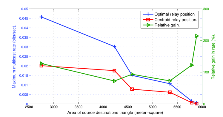
Figure 6: BRC with $n=2$ destinations. Rates for $r$ located at the centroid of $\triangle_{sd_{1}d_{2}}$, at the optimal position, and relative gain.

In this section, we present simulation results for the BRC with $n=2$ destinations. We compare the multicast rate obtained by optimizing the relay location and the source in addition to relay power allocations, with the case where the relay is located at a naive yet seemingly interesting position: the centroid of triangle $\triangle_{sd_{1}d_{2}}$ , and only the power allocations are optimized. The simulations are run for an increasing size of the area of $\triangle_{sd_{1}d_{2}}$ and a random network topology for each area is chosen.

Figure 6 shows the maximum multicast rate (blue and red) for optimal and centroid relay positions respectively. The SNR $\frac{P}{N_{0}}$ is normalized to 1. Note that the actual values of the rates are not as important because of the normalization, for higher power values, the rate would certainly have higher values. For increasing area of triangle $\triangle_{sd_{1}d_{2}}$, the maximum multicast rate tends to drop, which is due to the constrained power and larger distances, but the relative gain goes up. This implies that for farther placed nodes the sensitivity of the relay location is higher and can produce significant gains in rate for the optimal relay location. Its clear from the results in Figure 6 that the centroid is not the optimal location. The rise in the relative gain becomes very strong due to the fact that the low-SNR regime is more sensitive to the location of nodes (hence, distances) that determine the hyperarc rates in the limit of disappearing SNR as opposed to e.g. in high SNR regime, where a displacement of $\pm\epsilon$ for the location of $r$ would not effect the rate significantly.

V ARBITRARY CASE

In this section, we answer the same set of questions but for arbitrarily placed source and destination nodes. Almost all concepts can be carried over to, straightforwardly.

The steps of the pre-processing stage can be summarized as

Input: $\{s,T\}$ set of nodes with their cartesian coordinates.

1. Compute convex hull $\mathcal{C}$.

2. Compute $\mathcal{H}_{s}$, switch functions (using Lemma 2).

3. Compute the disjoint convex regions by superimposing all $k$-order Voronoi diagrams of $\mathcal{C}$.

4. Compute $\mathcal{H}_{r}$ (using relay hyperarc algorithm).

Output: $\mathcal{H}=\mathcal{H}_{s}\cup\mathcal{H}_{s}$.

Once we have $\mathcal{H}_{s}$ and $\mathcal{H}_{s}$, we can compute $\Omega=[1,|\mathcal{H}_{s}|\times|\mathcal{H}_{r}|]$. Ultimately, the optimization program could be stated as,

Program (D): $$\mbox{maximize }\left(g_{0}(x)\right)$$

subject to: $$g_{i}(x)\leq 1,\hskip 5.69054pti\in[1,k],$$ (35)

$$g_{j}(x)\leq 1,\hskip 5.69054ptj\in[k+1,K],$$

where, the constraints (35) are the posynomials constraints that can be transformed to convex convex constraints using GP and constraints (35) are the non-posynomial constraints that are approximated using $p$-norm approximation. The objective function $g_{0}(x)$ represents the multicast rate. In program (D), $x$ is a vector of variables.

Program (D), is an abstract representation of the actual program. Since, the program (D) is simply program (B) (but for arbitrary placement of destination nodes), the structure of (D) is the same as (B). The main difference is the pre-processing stage for the two cases, in this case which involves computation of $k$ nearest neighbor nodes and superimposing them to form disjoint regions in $\mathcal{C}$ for distinct $n$-nearest neighbors. We would like to note, that this computation, although polynomially bounded, can be heavy. There are many polynomial time algorithms in the literature of computational geometry that solve this problem efficiently, [23].

VI RESULTS AND CONCLUSION

A comprehensive and efficient solution is developed to model and answer the problem of optimal relay positioning so as to maximize the multicast rate from the source $s$ to the destination set $T$ in a low-SNR network. The proposed solution is a non-convex network optimization problem in its basic form that is difficult to solve. Using GP, switch functions and $p$-norm surrogate approximation we transform the problem to a convex approximation that can be solved using standard convex optimization algorithms.

To abridge, the important contributions of this work could be summed up in the following words: we present a comprehensive approach to determine the optimal relay position under the pretext of network optimization problem. Network topologies consisting single source, multiple destinations with the only intermediate node as relay are considered in complete generality on a $2$-D plane. Using superposition coding and frequency division we construct a wireline like hypergraph. The low-SNR hyperarc model using superposition coding provides an interference free network model that is easily scalable to complex network topologies. Using the tools of computational geometry and network optimization, we presented a network optimization framework based solution that is intuitive and easy to understand. Also, we show that positioning the relay optimally significantly affect the network performance.

In addition, the main causes for complexity in our approach are the pre-processing stage and the non-convexity arising from non-posynomial constraints upon GP transformation. The former reason could be somewhat tolerated, as generally for solving network planning problems heavy pre-processing is required. In contrast, in our case the pre-processing stage consists of polynomial time operations at the cost of only slight sub-optimality in approximation.

The questions our work answers are just a fraction of the interesting questions that it opens up. An interesting direction would be to extend this model to general multicommodity flow optimization problems involving more number of relay nodes. On the other hand, from the computational point of view, an interesting question is how we can efficiently build the exact number of paths essentially bringing down the size of the network optimization program. Finding other techniques to model this problem could be interesting, e.g. utilizing geometric properties of the problem and ways to bring down the computational complexity.

References

- [1] 3GPP. (2010, Mar.) Further advancements for EUTRA: Physical layer aspects. TR 36.814 V2.0.1 Tech. Spec.n Group Radio Access Network Rel. 9. 3GPP. [Online]. Available: http://www.3gpp.org/ftp/Specs/html-info/36814.htm
- [2] Y. Yang, H. Hu, J. Xu, and G. Mao, “Relay technologies for wimax and lte-advanced mobile systems,” IEEE Commun. Mag., vol. 47, no. 10, pp. 100–105, Oct. 2009.
- [3] D. Astely, E. Dahlman, A. Furuskar, Y. Jading, M. Lindstrom, and S. Parkvall, “Lte: the evolution of mobile broadband,” IEEE Commun. Mag., vol. 47, no. 4, pp. 100–105, Apr. 2009.
- [4] C. Shannon, “Communication in the presence of noise,” Proceedings of the IRE, vol. 37, no. 1, pp. 10–21, Jan. 1949.
- [5] R. S. Kennedy, Fading Dispersive Communication Channels. New York: Wiley-Interscience, 1969.
- [6] R. G. Gallager, Information Theory and Reliable Communication. New York: Wiley-Interscience, 1968.
- [7] I. Telatar and D. Tse, “Capacity and mutual information of wideband multipath fading channels,” IEEE Trans. Inform. Theory, vol. 46, no. 4, pp. 1384–1400, July 2000.
- [8] M. Médard and R. Gallager, “Bandwidth scaling for fading multipath channels,” IEEE Trans. Inform. Theory, vol. 48, no. 4, pp. 840–852, Apr. 2002.
- [9] S. Verdú, “Spectral efficiency in the wideband regime,” IEEE Trans. Inform. Theory, vol. 48, no. 6, pp. 1319–1343, June 2002.
- [10] V. Subramanian and B. Hajek, “Broad-band fading channels: signal burstiness and capacity,” IEEE Trans. Inform. Theory, vol. 48, no. 4, pp. 809–827, Apr. 2002.
- [11] D. S. Lun, M. Médard, and I. C. Abou-Faycal, “On the performance of peaky capacity-achieving signaling on multipath fading channels,” IEEE Trans. Commun., vol. 52, no. 6, pp. 931–938, June 2004.
- [12] L. Zheng and D. Tse, “Communication on the grassmann manifold: a geometric approach to the noncoherent multiple-antenna channel,” IEEE Trans. Inform. Theory, vol. 48, no. 2, Feb. 2002.
- [13] S. Ray, M. Médard, and L. Zheng, “On non-coherent MIMO channels in the wideband regime: Capacity and reliability,” IEEE Trans. Inform. Theory, vol. 53, no. 6, pp. 1983–2009, June 2007.
- [14] T. M. Cover, “Broadcast channels,” IEEE Trans. Inform. Theory, vol. 18, no. 1, Jan. 1972.
- [15] A. E. Gamal and T. M. Cover, “Multiple user information theory,” Proceedings of the IEEE, vol. 68, no. 12, pp. 1466–1483, Dec. 1980.
- [16] R. McEliece and L. Swanson, “A note on the wide-band gaussian broadcast channel,” IEEE Trans. Commun., vol. 35, no. 4, pp. 452–453, Apr. 1987.
- [17] R. G. Gallager, “A perspective on multiaccess channels,” IEEE Trans. Inform. Theory, vol. 31, no. 2, pp. 124–142, Mar. 1985.
- [18] N. Fawaz and M. Médard, “On the non-coherent wideband multipath fading relay channel,” in Proc. IEEE International Symposium on Information Theory, ISIT 2010, Austin, TX, USA, June 2010. [Online]. Available: http://arxiv.org/abs/1002.3047
- [19] M. Thakur and M. Médard, “On optimizing low SNR wireless networks using network coding,” in Proc. IEEE Global Communications Conference, Globecom 2010, Miami, FL, USA, Dec. 2010.
- [20] S. Boyd and L. Vandenberghe, Convex Optimization. New York: Cambridge University Press, Mar. 2004.
- [21] T. M. Cover, “Comments on broadcast channels,” IEEE Trans. Inform. Theory, vol. 44, no. 6, pp. 2524–2530, Oct. 1998.
- [22] F. P. Preparata and M. I. Shamos, Computational Geometry. Springer-Verlag, 1985.
- [23] H. Edelsbrunner, Algorithms in Combinatorial Geometry. Springer-Verlag, 1987.
- [24] D.-T. Lee, “On k-nearest neighbor Voronoi diagrams in the plane,” IEEE Transactions On Computers., vol. 31, no. 6, June 1982.
- [25] A. Lundell, J. Westerlund, and T. Westerlund, “Some transformation techniques with applications in global optimization,” Journal of Global Optimization, vol. 43, Mar. 2009.
- [26] J.-F. Tsai, M.-H. Lin, and Y.-C. Hu, “On generalized geometric programming problems with non-positive variables,” European Journal of Operational Research., vol. 178, Apr. 2007.
- [27] D. Li, “Zero duality gap in integer programming: P-norm surrogate constraint method,” Operations Research Letters., no. 25, June 1999.