Co–propagating Bose–Einstein Condensates and electromagnetic radiation: Emission of mutually localized structures

Abstract

Using a semi-classical model to describe the interaction between coherent electromagnetic radiation and a Bose-Einstein condensate in the limit of zero temperature, including the back action of the atoms on the radiation, we have analyzed the phenomenon of emission of solitary-like wave packets which can accompany the formation of mutually localized atom-laser structures.

I Introduction

With the realization of Bose-Einstein condensates (BEC) and of coherent atomic beams all the questions inherent to the manipulation of such systems have acquired a certain importance. In particular, early studies such as ref:first ; ref:zhang have started an interest in the manipulation of atomic structures via their interactions with coherent electromagnetic radiation. Not only these studies could be of importance for applications such as atom interferometry, they also offer a possible test of the analogies between optics and quantum matter waves. In fact, BECs provide us with a quantum system where matter waves can be realized on macroscopic scales and which, under the approximations of zero temperature, low densities, weak interactions and within the limits of validity of a mean field theory, is amenable to a mathematical description based on the Gross-Pitaevskii equation, completely akin to the basic equation of nonlinear optics, i.e. the nonlinear Schrödinger equation, ref:review . The Kerr-like nonlinearity is given for the atoms by the atom-atom interactions. It has been demonstrated that it is possible to reproduce typical optical and nonlinear optical phenomena with a a BEC, from the generation of solitons to four-wave mixing, from parametric amplification to second harmonic generation, to mention only a few of them (for a review, see ref:meystre and references therein). It is possible to push the analogy even further and consider the electromagnetic radiation as the medium that allows for nonlinear interactions between atoms as discussed initially in ref:first . This corresponds exactly to the optics case where the medium through which radiation propagates can bring about nonlinear effects for the electromagnetic field: Nonlinear effects in the dynamical evolution of the atoms and of the radiation are then a consequence of the atom-light interactions. Models of this interaction were presented by several authors, ref:zhang ; ref:models and Krutitsky et al., ref:krutitsky , gave a full derivation of the equations describing it starting from first principles within the framework of quantum field theory. This last work showed the emergence of a resonant nonlinear term in the system dynamics as a consequence of the laser-atom dipole-dipole interaction, besides the well known Kerr-like nonlinearity. The same equation for the atoms and consequently a coupled system of equations for the laser-atom system were rederived in ref:us1 , this time starting from a semi-classical theory. It was found there that the response of the ”medium”, that is of the laser radiation, to the dynamics of the condensate could play an important role in the coupled evolution and even allow for the formation of mutually localizd atom-laser structures capable of propagating with no changes in the atom density and laser intensity, in spite of the assumed repulsive atom-atom interaction. Such solitary-like structures are of interest bacause of their properties of self-localization and robust propagation and the effects of these interactions can be seen also in relation to the creation of meta-lenses and comoving potentials to refocus atom waves, ref:comoving . Their emerging as a result of the coupling during propagation of atoms and laser was studied in ref:us1 while the stationary states of the coupled system and their stability properties were introduced in ref:us2 . However, little is known about their actual mechanism of formation. In the optics case of a focusing nonlineariry, we would expect an initial bell-shaped structure to shed away the radiation which cannot be accomodated and to adjust asymptotically to a soliton wave. It is interesting to see whether the same happens in the present case of coupled atom-laser propagation and how, since the coupling may lead to novel effects. We have therefore studied numerically the process through which such coupled soliton-like objects are formed evidentiating the occurrence of a phenomenon reminiscent of soliton emission in nonlinear optics, ref:emission . In fact, the equations analyzed here, predict the formation of solitary-like structures for both atoms and light which can move away from the region where they were generated. Although in our case there is no external trapping but only the self-consistent interaction of atoms and laser, these results are suggestively similar to escaping solitons described and observed in completely different environments, for instance in nematic liquid crystals, ref:escaping .
We will breafly review the basic physics of the semi-classical model and the limitations to be considered in Sec.II. Sec.III presents an investigation of the initial evolution of the coupled system which will than be studied numerically in Sec.IV.

II Semi-classical model and set up of the problem

The basic physics of atom-laser interactions in the simplest dipole approximation is given by photons exciting atoms which in turn re-emit photons absorbed by other atoms, thus giving rise to a long-range interatomic interaction, ref:cohen . Details of the semi-classical derivation of both the atom and the laser equations are given in ref:us1 ; ref:us2 , here we will only briefly review the two model equations and re-introduce the notation. In a semi-classical derivation, the force exerted by the light on the atoms is written as the gradient of a potential and this potential is used as the atom-laser interaction term in the Hamiltonian for the atoms Schrödinger equation. Such force term is a generalization of the ponderomotive force and takes into account the possibility of an inhomogenoeus gas. The existence of stationary solutions is physically crucial so we will study a far-off resonant monochromatic field ${\bf{E}}({\bf{r}},t)=Re[{\boldsymbol{\mathcal{E}}}({\bf r})\exp(-i\omega_{L}t)]$ (where ${{\boldsymbol{\mathcal{E}}}({\bf r})}$ is the complex amplitude of the laser field). The time averaged force (over laser cycles) is ${\bf F}=\frac{1}{16\pi}\nabla\left[|{\bf{E}}|^{2}\frac{\partial\epsilon}{\partial n}\right]=-{\boldsymbol{\nabla}}V_{d}.$ Here $\epsilon(\omega,n)$ is the medium dielectric constant with atom density $n$ and is given by $\epsilon(\omega,n)=1+\frac{4\pi\alpha n}{1-\frac{4\pi}{3}\alpha n},$ where, as derived from quantum theory, $\alpha(\omega)=-d^{2}/\hbar\Delta$ is the atomic polarizability at the laser frequency $\omega_{L}$, with $\Delta=\omega_{L}-\omega_{a}$ being the detuning from the nearest atomic resonance frequency $\omega_{a}$, and $d$ is the dipole matrix element of the resonant transition,ref:krutitsky ; ref:born . The relative semplicity of the semi-classical derivation comes at the price of restricting the validity of the model to a well defined range of parameters: The concept of force is purely classical, therefore quantum fluctuations, stochastic heating and any incoherent process are to be neglected. This limits the validity of this model to large detunings $|\Delta|\gg\omega_{a},\Gamma$ ($\Gamma$ is the atoms natural line width). Under these limitations, the potential $V_{d}$ can be inserted into the atom Gross–Pitaevskii equation where it describes the laser-induced dipole-dipole interaction between the atoms:

$$i\hbar\frac{\partial\Psi}{\partial t}=\hat{H}_{0}\Psi+\left[U_{0}|\Psi|^{2}-\frac{\alpha}{4}\frac{|{\bf{E}}|^{2}}{\left(1-\frac{4\pi}{3}\alpha|\Psi|^{2}\right)^{2}}\right]\Psi.$$ (1)

Here $\hat{H}_{0}$ is the linear single-particle Schrödinger Hamiltonian, the wave function $\Psi$ is normalized as $N=\int|\Psi|^{2}d{\bf r}$ with $N$ denoting the total number of atoms, so that the gas density is $n=|\Psi|^{2}$, $U_{0}=4\pi\hbar^{2}a_{s}/m$, $m$ is the atom mass and $a_{s}$ is the $s$–wave scattering length (which will be assumed positive as for repulsive atom-atom interactions). Furthermore, since we are interested in the stationary behaviour of the system and we have already assumed a stationary form for the electromagnetic field, we will consider $\Psi({\bf{r}},t)=\Phi({\bf{r}})\exp(-i\omega_{a}t)$. The atom equation was already derived in ref:krutitsky within a fully quantum model and it is important to underline that, once the limitations of the semi-classical reasoning are taken into account, the two derivations lead to the same equation.
To describe the role played by the electromagnetic field and the effect of the atoms on such field, it is necessary to include a field equation. Maxwell’s equations for the propagation of radiation in a medium, ref:born ; ref:jackson ; ref:us1 , yield a wave equation which, under the assumption of $L_{n}\gg\lambda_{L}$ or ${\boldsymbol{\nabla}}\epsilon\cdot{\bf{E}}\simeq 0$ ($L_{n}$ is the characteristic length scale of transverse density modulations and $\lambda_{L}$ is the radiation wavelength), gives the three scalar equations ($\omega_{L}=k_{L}c$)

$$\nabla^{2}{\boldsymbol{\mathcal{E}}}+k_{L}^{2}\left(1+\frac{4\pi\alpha|\Phi|^{2}}{1-\frac{4\pi}{3}\alpha|\Phi|^{2}}\right){\boldsymbol{\mathcal{E}}}=0.$$ (2)

When the input field distributions do no match the exact stationary solutions (which can be found numerically, ref:us2 ), propagation effects of some sort are to be expected. As demonstrated in ref:us1 , in the case of red detuning, the system settles down asymptotically to a stationary state with mutually localized atom-laser structures: Starting from a gaussian atom density profile and a super-gaussian laser intensity one, the interaction leads to the formation of two bell-shaped structures which propagate unchanged thereon. This means that atoms and radiation in excess will be shed away, which is the process we would like to elucidate here. Choosing $z$ as the propagation coordinate and limiting the investigation to slow envelope variation, we consider

$${\boldsymbol{\mathcal{E}}}({\bf{r}}) = a(x,z)\exp(ik_{L}z){\bf{e}},$$ (3)

$$\Phi({\bf{r}}) = \psi(x,z)\exp(ik_{a}z),$$ (4)

where $x$ denotes the dimension transverse to the propagation direction $z$ (one transverse dimension only for simplicity), ${\bf e}$ is the polarization vector of the field and $k_{a}$ is the atom wave number. The coupled system of equations (1), (2), can then be written in normalized variables as

$$i\mu\frac{\partial\tilde{\psi}}{\partial\tilde{z}}=-\frac{1}{2}\frac{d^{2}\tilde{\psi}}{d\tilde{x}^{2}}+\frac{1}{2}\beta_{coll}|\tilde{\psi}|^{2}\tilde{\psi}-\frac{s}{2}\frac{|\tilde{a}|^{2}}{\left(1-s|\tilde{\psi}|^{2}\right)^{2}}\tilde{\psi}$$ (5)

$$i\frac{\partial\tilde{a}}{\partial\tilde{z}}=-\frac{1}{2}\frac{d^{2}\tilde{a}}{d\tilde{x}^{2}}-\frac{3s}{2}\frac{|\tilde{\psi}|^{2}\tilde{a}}{1-s|\tilde{\psi}|^{2}},$$ (6)

where the following normalisation has been used: $\tilde{x}={x}k_{L}$, for the atom wave function $\tilde{\psi}=\psi/\psi_{*}$ with $(4\pi|\alpha|/3)\psi_{*}^{2}=1$, for the laser $\tilde{a}=a/a_{*},$ with $m|\alpha|a_{*}^{2}/(2\hbar^{2}k_{L}^{2})=1$, $s=sign(\alpha)$, $\mu=k_{a}/k_{L}$ (for simplicity we will assume $\mu=1$ hereafter) and $\beta_{coll}=6a_{s}/(k_{L}^{2}|\alpha|)$. The tilde will be dropped hereafter unless otherwise stated. The red detuning case studied here will correspond to $s=+1$. Notice that no mutual localization is possible in the blue detuning case. While the classical description for the laser field is justified by the choice of the intensity regime, for a mean field model to be valid for the atom wave function, we must consider not only a zero temperature limit but also a low density limit with $na_{s}^{3}\ll 1$, see ref:review . Furthermore, a low density regime is required in order to avoid the singularity of the model and consequent spurious collapse-like phenomena.

III Initial evolution

As done previously, we will start assuming an initial laser intensity profile in super-gaussian form much wider than the gaussian initial atom density profile, both of them definitely different from the stationary solutions of the system thus ensuring a dynamical evolution:

$$\psi(x,0) = \psi_{0}e^{\left(-x^{2}/2d_{a}^{2}\right)}$$ (7)

$$a(x,0) = a_{0}e^{-\left(x^{2}/2d_{L}^{2}\right)^{g}}$$ (8)

where $g$ is the supergaussian parameter ($g=10$ in the simulations). The flat-top laser profile eliminates gradient forces on the atoms at the very initial stage. However, the flat top is immediately modified due to the natural evolution of the system and the initial steps will be the seed of the subsequent structure generation. The atoms will imprint a chirp on the laser with the effect of creating a central intensity peak with two lateral throughs, ref:us1 . This can be formally seen via a perturbative solution of the first propagation stage (i.e. for $z\ll\lambda_{L}$). With $|\psi|^{2}\ll 1$, the denominators in Eqs.(5) and (6) can be expanded keeping terms up to the order $\sim|\psi|^{2}$. Separating amplitude and phase as $a(x,z)=A(x,z)\exp(i\theta(x,z)),\psi(x,z)=B(x,z)\exp(i\phi(x,z))$ the two equations give, upon separation of real and imaginary parts,

$$\left\{\begin{array}[]{l}\frac{\partial\phi}{\partial z}=\frac{1}{2}\left[\frac{1}{B}\frac{\partial^{2}B}{\partial x^{2}}-\left(\frac{\partial\phi}{\partial x}\right)^{2}\right]+\frac{A^{2}}{2}-B^{2}\left(\frac{\beta}{2}-A^{2}\right),\\ \frac{\partial B^{2}}{\partial z}=-\frac{\partial}{\partial x}\left(B^{2}\frac{\partial\phi}{\partial xi}\right),\\ \frac{\partial\theta}{\partial z}=\frac{1}{2}\left[\frac{1}{A}\frac{\partial^{2}A}{\partial x^{2}}-\left(\frac{\partial\theta}{\partial x}\right)^{2}\right]+\frac{3}{2}B^{2},\\ \frac{\partial A^{2}}{\partial z}=-\frac{\partial}{\partial x}\left(A^{2}\frac{\partial\theta}{\partial x}\right).\end{array}\right.$$ (9)

Consider a perturbative expansion $F(x,z)=F_{0}(x)+F_{1}(x)z+F_{2}(x)z^{2}$ and $G(x,z)=G_{1}(x)z+G_{2}(x)z^{2}$ up to second order in $z$ where $F$ stands for the functions $A$ and $B$ while $G$ stands for $\theta$ and $\phi$ and the zero-th order terms are the initial functions (7) and (8). Identifying powers of $z$, a solution is obtained for the amplitudes:

$$A^{2}=A_{0}^{2}(x)\left[1-\frac{3}{2}\frac{B_{0}^{2}(x)}{d_{a}^{2}}\left(\frac{2x^{2}}{d_{a}^{2}}-1\right)z^{2}\right],$$ (10)

$$B^{2}=B_{0}^{2}(x)\left[1+\frac{1}{2}\frac{\beta^{\prime}(x)}{d_{a}^{2}}B_{0}^{2}(x)\left(\frac{2x^{2}}{d_{a}^{2}}-1\right)z^{2}-\frac{z^{2}}{2d^{4}}\right]$$

where $\beta^{\prime}(x)=\beta-2A_{0}^{2}(x)$. This solution has the features observed in the initial evolution of the coupled system: The laser intensity profile changes in such a way as to peak in the center and at the same time two troughs are created on each side of the rising peak. The atom density profile shows the well known nonlinear defocusing behaviour - the center is depressed and two humps are created on both sides of the depression. This is the beginning of the creation of the stable mutually localized structures discussed in ref:us1 , in a soliton-like process the nonlinearity in the atom equation can act as a self-generated trapping potential for the BEC.

IV Structure emission

As a consequence of the initial evolution stage, provided the strenght of the focusing dipole-dipole interaction and that of the defocusing collisional nonlinearity are initially not completely out of balance, some atoms start to broaden away from the central structure while a part of the initial distribution remains trapped there. The radiation reacts to this process because of the dependence of the refactive index on the density profile and part of it is focused around the peak of the atom density. However, if the trap induced by the laser is much wider than the atom wave function, the atoms lost from the central core can still be trapped. What initially was a hump of disperding atoms, can get trapped in a secondary self-generated potential well and induce mutual localization on the wings. The generation of these secondary mutually localized structures, keeping the initial laser with and peak intensity fixed, should depend on having enough atoms escaping from the central peak since the escaping atoms must affect the laser wings to provoke the formation of the secondary trap. Therefore we have numerically studied the coupled evolution of (7) and (8) for fixed $d_{a}=5\lambda_{L},d_{L}=8d_{a}$ and fixed $a_{0}=0.1346$ corresponding to an initial peak laser intensity of $0.0153$ mW/cm², but varying $\psi_{0}$. In the simulations we have $\beta\simeq 38$ corresponding for instance to a detuning of $100$ times the decay rate for ⁸⁷Rb atoms and $s=+1$.
As anticipated, for low $\psi_{0}$, only a central density peak remains, a phenomenon studied in ref:us1 . The central atoms affect the laser profile which creates a trapping potential. The atoms that escape this trap are not enough to modify the natural evolution of the laser wings which undergo well known modulations before diffracting away. Increasing $\psi_{0}$, the central structure generated by the system will be obviously modified, the balance of repulsive collisional interactions and attractive dipole forces has changed. Furthermore, the effect of escaping atoms becomes stronger to the point that the same trapping mechanism can now be realized on the sides of the central peak. Fig.1 shows the results of such an interaction for two values of $\psi_{0}.$ The laser, as one would expect, forms analogous localized structures in correspondence of the atom density peaks. There is actually a formation of localized structures even for low $\psi_{0}$, the very low density of escaping atoms can focus extremely weak laser peaks, the process creates continuous families of mutually localized solutions. However, for low $\psi_{0}$ they are hardly visible.

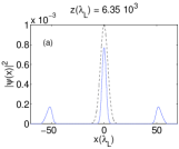
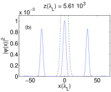
Figure 1: Structure formation for (a) $\psi_{0}=0.0316$ (corresponding to an initial peak atom density $n_{0}=1.7\,10^{19}\textrm{ m}^{-3}$) and (b) $\psi_{0}=0.06645$ (corresponding to $n_{0}=7.51\,10^{19}\textrm{m}^{-3}$). Dotted line: initial density distriubution. The propagation distance is indicated on the plots. All other parameters as specified in the text. All quantities normalized as in the text.

What is interesting about these structures is their fate. They are self-consistently formed due to the effect they have on the laser radiation. Atoms focus the radiation, the radiation in turns exerts a focusing action on the atoms counterbalanced by their own defocusing interaction and their kinetic energy. During the initial transient, which lasts until the atom-laser structures are mutually adjusted to their own localized form, the lateral peaks are oscillating around the point where they have been trapped. They are kept there by the presence of the laser trap, laser wings have not yet completely adjusted to the newly born structures and they still act as an external trap for the atoms. Figs.2(a) and (b) show the intermediate stage of this transient for the same paramaters as in Fig.1(b). The structures are oscillating within the laser-induced trap which is being formed, Figs.2(c) and (d), and once the laser has completely adjusted nothing keeps the atom-laser peaks oscillating around a fixed position anymore and the structures are free to move away, Figs.2(e) and (f). For the parameters of Fig.2, they are ejected from the initial interaction region and proceed propagating with constant velocity as solitary-like waves. This could be explained by the repulsion due to the central peak: the two lateral peaks cannot proceed moving inward because they cannot overcome the repulsive barrier due to the central one.(???????)

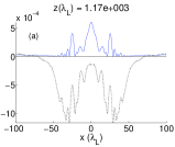
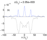
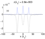
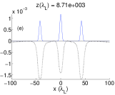
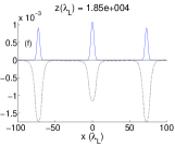
Figure 2: Details of the process of structure formation for $\psi_{0}=0.06645$ ($n_{0}=7.51\,10^{19}\textrm{m}^{-3}$). Solid line: atom wave function, dotted line: laser-induced potential acting on the atoms (divided by 10 to make the figure more easily readable). The propagation distance is indicated on the plots. All other parameters as specified in the text. All quantities normalized as in the text.

The position of the lateral peaks as a function of the propagation distance for the same parameters of Fig.2 is shown in Fig.3(a), from which it is clear that, after an initial transient during which it is quite difficult to keep track of the structures’ positions, the two “jets” are propagating at constant velocity. It is also evident how laser and atoms jets move together. Fig.3(b) shows the peak value of the atom density of the emitted structures which tend to stabilize on a stationary value.

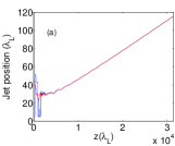
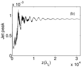
Figure 3: (a) Emitted structure position versus propagation distance for $\psi_{0}=0.06645$ ($n_{0}=7.51\,10^{19}\textrm{m}^{-3}$). Red: laser jet position; blue: atom jet position. (b) Peak atom density of the emitted structures for the same case. All quantities normalized as in the text. (Color on line.)

In a way, this phenomenon is reminiscent of the emission of solitons engeneered in nonlinear optics with the aim for instance of implementing all-optical switching and directional couplers, ref:emission . Whereas in the optics case the emission is stimulated only on one side, we obtain two moving structures because of the symmmetry of the configuration. We must underline that we refer to the emitted structures as solitary-like waves because of their ability to propagate with unchanged shaped but we have not yet proved their collisional properties, preliminary results indicate a behaviour strongly suggestive of a soliton-like nature.
The analogy is also suggestive of the possibility of soliton steering. In fact, the properties of the structures ejected (peak density, velocity and number of jets) depend on the initial conditions. Therefore, changing the initial value of $\psi_{0}$, we have found jets emitted at different angles with respect to the propagation direction $z$ and with different peak densities and peak laser intensities, as can be seen from Fig.4 which shows jet positions for a few different cases.

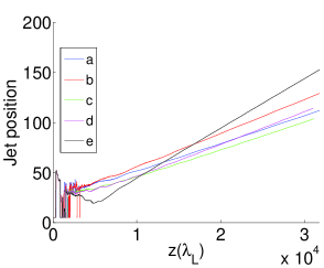
Figure 4: Jet positions for different initial values of the atom peak density $\psi_{0}$. All other parameters are the same as for Fig.1. (a) $\psi_{0}=0.052$, (b) $\psi_{0}=0.054$, (c) $\psi_{0}=0.0662$, (d) $\psi_{0}=0.0664$, (e) $\psi_{0}=0.0668$. All quantities normalized as in the text. (Color on line.)

This last figure also shows the anomalous behaviour of the structures emitted starting from $\psi_{0}=0.0668$. They initially move clearly inwards before being ejected. For growing initial peak density, there seems to be a stronger central trapping capable to attract the lateral peaks towards the center. Notice from Fig.4 how, for higher initial $\psi_{0}$ the jets tend to be born closer and closer to the central peak, where they are likely to experience a stronger interaction with it, due to a larger overlap (compare cases (a) and (b) in that figure with cases (c) and (d) which have larger $\psi_{0}$). There is a critical combination of parameters, which in our case occurs for $\psi_{0}=0.0669$, such that the two jets are drawn backwards until they collide and fuse at the center, Fig.5. It is known that the result of a collision between two solitons depending on the relative phase can lead to the fusion of the two objects, ref:collision and references therein, however the nature of the collision within the model presented here needs further studies. After the merging, the remaining central peak stabilizes and does not undergo any dynamical changes anymore but it is very likely that such a structure will not be realized due to the extra-effects that are not considered within this model and that could play an important role during the collision.

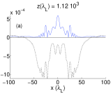
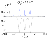
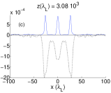
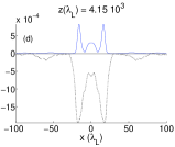
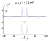
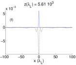
Figure 5: Propagation and fusion for $\psi_{0}=0.0669$ ($n_{0}=7.62\,10^{19}\textrm{m}^{-3}$). Solid line: atom wave function, dotted line: laser-induced potential acting on the atoms (divided by 10 to make the figure more easily readable). Propagation distance as indicated on the plots. All quantities normalized as in the text.

For higher values of $\psi_{0}$ no central peak is left while two lateral peaks are again symmetrically ejected. This could suggest an instability of the central peak as a possible explanation of the merging shown by the previous case. If the central peak is unstable against diffraction/defocusing and the laser-induced force is not able to keep it trapped, its atoms will broaden away with two possible outcomes for the jets: Either the repulsive interaction between the jets and the centrally disperding atoms is not strong enough to prevent the jets from merging in the center, or it is important enough to push them away, compare Fig.6 and 5.

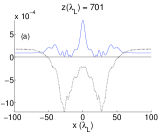
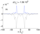
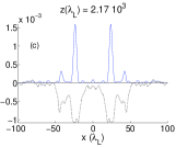
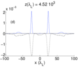
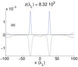
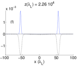
Figure 6: Structure emission for $\psi_{0}=0.092$ ($n_{0}=7.62\,10^{19}\textrm{m}^{-3}$). Solid line: atom wave function, dotted line: laser-induced potential acting on the atoms (divided by 10 to make the figure more easily readable). Propagation distance as indicated on the plots. All quantities normalized as in the text.

It is interesting to notice how the integral of the jets wavefunction ($N=\int_{-\infty}^{\infty}|\psi(x)|^{2}\,dx$ in Fig.7) seems to tend to a finite value as a function of the integral of the initial wavefunction ($N_{0}$ in Fig.7).

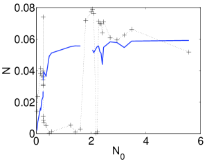
Figure 7: Integral of the jets wavefunctions $N=\int_{-\infty}^{\infty}|\psi(x,z\rightarrow\infty)|^{2}\,dx$ (solid line) and of the central peak wavefunction (dotted line) versus the integral of the initial wavefunction $N=\int_{-\infty}^{\infty}|\psi(x,z=0)|^{2}\,dx$. The points were the solid line is broken correspond to merging and fusion and therefore no emission of jets at all. All quantities normalized as in the text.

This would be acceptable from the point of view of soliton behavior: The emitted solitary-like structures can accomodate a given number of atoms, atoms in excess will go and form extra jets, an example is shown in Fig.8.

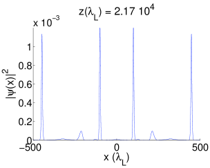
Figure 8: Structures emitted for $\psi_{0}=0.2$ ($n_{0}=6.81\,10^{20}\textrm{m}^{-3}$). Propagation distance as indicated on the plot. All quantities normalized as in the text.

A final note concerns one more analogy with an optical soliton behaviour. It seems in fact possible to excite a structure very similar to the bound system observed for optical solitons in which two pulses perform an oscillatory motion by bouncing back and forth in their own potential well, ref:collision . In a repeated dance, under particular conditions, the optical solitons pass through each other, move apart and come to a halt to move back together. This is what can be seen for a given choice of initial parameters for the system under analysis here. Fig.9 shows the value of the atom density at $x=0$ as a function of the propagation distance for $\psi_{0}=0.196$ and oscillations which would agree with the presence of a bound soliton state are quite evident. Corresponding snapshots are given in Fig.10.

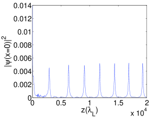
Figure 9: Evolution of the central atom density calculated as $|\psi(x=0)|^{2}$ as a function of the propagation distance for $\psi_{0}=0.196$ ($n_{0}=6.54\,10^{20}m^{-3}$). All quantities normalized as in the text.

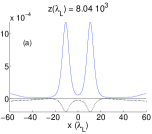
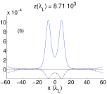
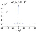
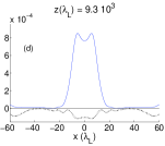
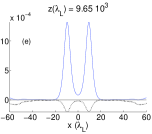
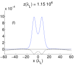
Figure 10: Snapshots of the evolution of the atom wavefunction for $\psi_{0}=0.196$ ($n_{0}=6.54\,10^{20}m^{-3}$). Propagation distance as given in the plots. All quantities normalized as in the text.

V Conclusions

In conclusion, proceeding from the idea that laser-BEC dipole-dipole interactions can lead to mutually localized structures, we have analyzed in detail the mechanism of formation of such structures concentrating on the process through which the structures shed away the extra atoms and extra radiation. Numerical simulations seem to indicate the possibility of generating and emitting secondary solitary-like wave packets in a jet-like fashon. Although the model used here is strongly simplified and any comparison with experiment will require major refinements, the equations we have used enlighten the main physical effects and it seems possible to choose parameter regimes in which the effects neglected here will not destroy these results. This processes could be a further evidence of the analogy between matter waves and optical waves and even open the discussion about applications such as soliton stirring in BECs.

Acknwledgment

F.C. would like to acknowledge the hospitality of the department of Radio and Space Physics of Chalmers University of Technology during the preparation of this work.

References

- (1) G. A. Askhar’yan Zh. Eksp. Teor. Fiz. 42 1567 (1962) [Sov. Phys JETP 15 1088 (1962)]; A. Ashkim Phys. Rev. Lett. 25 1321 (1970); Yu. L. Klimontovich and S. N. Luzgin JETP Lett. 30 610 (1979).
- (2) W. Zhang and D. F. Walls, Quantum Opt. 5, 9, (1993); M. Lewenstein, Li You, J. Cooper and K. Burnett, Phys. Rev. A, 50, 2207 (1994); J. J. Javanainen, Phys. Rev. Lett.72, 2375 (1994).
- (3) F. Dalfovo, S. Giorgini, L. P. Piatevskii and S. Stringari, Rev. Mod. Phys. 71 463–512 (1999); A. J. Leggett, Rev. Mod. Phys. 73 307–356 (2001); C. J. Pethick and H. Smith Bose-Einstein condensation in dilute gases (Cambridge University Press, Cambridge, 2004).
- (4) P. Meystre, J. Phys. B: At. Mol. Opt. Phys. 38, S617-S628 (2005).
- (5) M. Saffman, Phys. Rev. Lett. 81, 65, (1998); N. N. Rozanov, N. V. Vysotina and A. G. Vladimirov, JETP 91, 1130, (2000).
- (6) K. V. Krutitsky, F. Burgbacher, and J. Audretsch, Phys. Rev. A 59, 1517 (1999).
- (7) F. Cattani, A. Kim, D. Anderson, and M. Lisak, J. Phys. B: At. Mol. Opt. Phys. 43, 085301, (2010).
- (8) R. Mathevet, J. Robert, and J. Baudon, Phys. Rev. A61, 033604 (2000);
- (9) F. Cattani, D. Anderson, A. Kim and M. Lisak, JETP Lett. 81, 561 (2005); F. Cattani, V. Geyko, A. Kim, D. Anderson, and M. Lisak, Phys. Rev. A 81, 043623 (2010).
- (10) E. M. Wright, D. R. Heatley, and G. I. Stegeman, Phys. Rep. 194, 309, (1990).
- (11) G. Assanto, A. A. Minzoni, M. Peccianti, and N. F. Smyth, Phys. Rev. A 79, 033837 (2009).
- (12) C. Cohen-Tannoudji, J. Dupont-Roc, and G. Grynberg Atom-Photon Interactions (Wiley, Berlin, 1998).
- (13) M. Born and E. Wolf, Principles of Optics: Electromagnetic Theory of Propagation, Interference and Diffraction of Light (Cambridge University Press, Cambridge, 1999).
- (14) J. D. Jackson, Classical Electrodynamics (Wiley, New York, 1975).
- (15) J. P. Gordon, Opt. Lett. 8, 596 (1983). M. Karlsson, D. Anderson, A. Höök, and M. Lisak, Phys. Scr. 50, 265, (1994); O. Bang, L. Berge’, and J. Juul Rasmussen, Phys. Rev. E 59, 4600, (1999); W. Krolikowski, B. Luther-Davies, C. Denz, and T. Tschudi, Opt. Lett. 23 97, (1998); N. H. Seong and Dug Y. Kim, Opt. Lett. 27, 1321, (2002).