Quantum realization of extensive games

Abstract

We generalize a concept of classical finite extensive game to make it useful for application of quantum objects. The generalization extends a quantum realization scheme of static games to any finite extensive game. It represents an extension of any classical finite extensive games to the quantum domain. In addition our model is compatible with well-known quantum schemes of static games. The paper is summed up by two examples.

1 Introduction

The quantum game theory is based on the combination of game theory and quantum information. From the mathematical point of view an arena of a quantum game is a tensor product of multidimensional Hilbert spaces where unitary operators acting on fixed vectors from these spaces are treated as actions taken by players [2]. The paper [1] deserves the special attention. In this paper the authors introduce the model of a quantum realization of any static 2$\times$2 game. Another important paper is [5] where the authors show an alternative model of a quantum static game. Quantum game theory goes beyond static games. Among recent papers there can be found problems of duopoly, poker games, repeated games, etc., played in the quantum domain. Motivation for our research has been a scientific niche that remains in an area of quantum extensive games. Our paper is entirely dedicated to this topic entirely.

We decided to remind in next section basic notions of game theory which will be necessary in the sequel. Readers who are not familiar with game theory are encouraged to consult [6] and [12]. Necessary elements of quantum information can be found in [4] and [11].

2 Preliminaries of game theory

This section starts with defining a game in an extensive form. In all cases when we refer to the concept of the game, we have in mind finite games that is, games with finite set of strategies for each player.

Definition 2.1

[12] Let the following components be given:

1. A finite set $N=\{1,2,\dots,n\}$ of players.

2. A set $H$ of finite sequences that satisfies the following two properties:

   1. The empty sequence $\emptyset$ is a member of $H$.

   2. If $(a_{k})_{k=1,2,\dots,K}\in H$ and $L<K$ then $(a_{k})_{k=1,2,\dots,L}\in H$.

   Each member of $H$ is a history and each component of a history is an action taken by a player. A history $(a_{1},a_{2},\dots,a_{K})\in H$ is terminal if there is no $a_{K+1}$ such that $(a_{1},a_{2},\dots,a_{K},a_{K+1})\in H$. The set of actions available after the nonterminal history $h$ is denoted $A(h)=\{a\colon(h,a)\in H\}$ and the set of terminal histories is denoted $T$.

3. The player function $P\colon H\setminus T\rightarrow N\cup c$ that points to a player who takes an action after the history $h$. If $P(h)=c$ then chance (the chance-mover) determines the action taken after the history $h$.

4. A function $f_{c}$ that associates with each history $h$ for which $P(h)=c$ an independent probability distribution $f_{c}(\cdot|h)$ on $A(h)$.

5. For each player $i\in N$ a partition $\mathcal{I}_{i}$ of $\{h\in H\setminus T:P(h)=i\}$ with the property that for each $I_{i}\in\mathcal{I}_{i}$ and for each $h$, $h^{\prime}$ $\in I_{i}$ an equality $A(h)=A(h^{\prime})$ is fulfilled.

The extensive game form is a tuple $(N,H,P,f_{c},\{\mathcal{I}_{i}\}_{i\in N})$.

Each element $I_{i}$ of the partition $\mathcal{I}_{i}$ is called an information set for a player $i$. The partition of set $H\setminus T$ into the information sets corresponds to the state of players’ knowledge. A player who makes move after certain history $h$ belonging to an information set from $\mathcal{I}_{i}$, knows that the current course of the game takes the form of one of histories being part of $I_{i}\in\mathcal{I}_{i}$. She does not know, however, if it is the history $h$ or the other history from $I_{i}$.

The complete description of a game also requires a utility function for each player $i$ to be defined. The full description of this function can be found in [6] and [12]. For our purpose it suffices to understand the utility function as a function assigning a real number to each terminal history. This number reflects preference of the $i$-th player with respect to particular terminal history.

Definition 2.2

[12] The extensive game form together with a collection $\{u_{i}\colon i\in N\}$ of utility functions $u_{i}\colon T\to\mathbb{R}$ is called the extensive game.

Although an extensive game from definition 2.2 describes every extensive game, our deliberations focus on games with perfect recall - this means games in which at each stage every player remembers all the information that she knew earlier and all of her own past moves. Further in the article if there is need to depict utility values (payoffs) for all players, we shall consider the utility function as function $u:T\to R^{n}$ defined as $u(h)=(u_{i}(h))_{i=1,2,\dots,n}$.

A game as a mathematical model can be described in algebraic language, thereby including a concept of isomorphism. Static game is defined only by a set of players $N$, collection of sets of strategies $\{S_{i}\}_{i\in N}$ and a utility function $u\colon\prod_{i=1}^{n}S_{i}\to R^{n}$. For this reason games: $(N,\{S_{i}\}_{i\in N},u)$ and $(N,\{S^{\prime}_{i}\}_{i\in N},u^{\prime})$ are isomorphic iff there exists bijection $\zeta\colon\prod_{i=1}^{n}S_{i}\to\prod_{i=1}^{n}S^{\prime}_{i}$ such that $u(s)=u^{\prime}(\zeta(s))$. The players who are taking part in some game cannot notice that they are playing indeed some of its isomorphic equivalents. Contrary to static games, the notion of isomorphism of extensive games is more complex.

Definition 2.3

The games in the form of tuples $(N,H,P,f_{c},\{\mathcal{I}_{i}\}_{i\in N},\{u_{i}\}_{i\in N})$ and $(N^{\prime},H^{\prime},P^{\prime},f^{\prime}_{c},\{\mathcal{I}^{\prime}_{i}\}_{i\in N},\{u^{\prime}_{i}\}_{i\in N})$ are called isomorphic, if there exists a bijective function $\xi\colon H\to~{}H^{\prime}$ that satisfies following conditions:

1. $\xi(\emptyset)=\emptyset^{\prime}$

2. $\forall_{h\in H\setminus T}$ $\bigl{(}\xi(h,a)=(h^{\prime},a^{\prime})\Rightarrow\xi(h)=h^{\prime}\bigr{)}$,

3. $\forall_{h\in H\setminus T}$ $P(h)=P^{\prime}(\xi(h))$

4. $\forall_{h\colon P(h)=c}$ $f_{c}(\cdot|h)=f^{\prime}_{c}(\cdot|\xi(h))$,

5. $\forall_{i\in N}\forall_{I_{i}\in\mathcal{I}_{i}}$ $\xi(I_{i})=I^{\prime}_{i}$,

6. $\forall_{h\in T}\forall_{i\in N}$ $u_{i}(h)=u^{\prime}_{i}(\xi(h))$.

We realize that the above defined notion of isomorphic games contains very restrictive conditions. According to the definition mentioned above, isomorphic games differ only by marks of all their components. The case of two games in which one of them will be modified by addition only one action $a_{1}$ of some player to the beginning history $\emptyset$ so that $A(\emptyset)=\{a_{1}\}$, does not satisfy the conditions of Definition 2.3.

The notions: action and strategy mean the same in static games, because the players choose their actions once and simultaneously. In the majority of extensive games players can make their decision about an action depending on all the actions taken previously by themselves and also by all the other players. In other words, players can have some plans of actions at their disposal such that these plans point out to a specific action depending on the course of a game. Such a plan is defined as a (pure) strategy in an extensive game.

Definition 2.4

[12] A strategy $s_{i}$ of player $i$ in a game $(N,H,P,f_{c},\{\mathcal{I}_{i}\}_{i\in N},u)$ is a function that assigns an action in $A(I_{i})$ to each information set $I_{i}\in\mathcal{I}$.

A sequence of strategies of all players $s=(s_{1},s_{2},\dots,s_{n})$ is called a profile of the strategies. Each profile $s$ determines unambiguously (if the chance mover has been excluded) some terminal history and each of its subhistories. However, for a fixed history $h$ there may exist a lot of strategies’ profiles which generate $h$. Generally:

Definition 2.5

[12] A strategy $s_{i}$ of a player $i$ is consistent with some history $h=(a_{1},a_{2},\dots,a_{k})$ if for every (strict) subhistory $(a_{1},a_{2},\dots,a_{l})$ of $h$ for which $P(a_{1},a_{2},\dots,a_{l})=i$ the condition $s_{i}(a_{1},a_{2},\dots,a_{l})=a_{l+1}$ is fulfilled. We define a profile $s=(s_{i})_{i=1,2,\dots,n}$ to be consistent with $h$ iff for every player $i$, $s_{i}$ is consistent with $h$.

Definitions 2.4 and 2.5 imply that any extensive game defined by Definition 2.2 induces some static (strategic) game $(N,\{S_{i}\}_{i\in N},u)$. Then for each $i\in N$ a set $S_{i}$ is the set of all possible functions defined by Definition 2.4. The utility function $u$ is the same as the one in the extensive game but is redefined from a domain $T$ to the domain $\prod_{i=1}^{n}S_{i}$ using the notion defined in Definition 2.5. It follows that notions assigned to static games are used in extensive games. One of these most important notions is a notion of an equilibrium introduced by John Nash in [7]:

Definition 2.6

Let mark by $(N,S_{i},\{u_{i}\}_{i\in N})$ a strategic form of an extensive game with perfect recall. A profile of strategies $(s^{*}_{1},s^{*}_{2},\dots,s^{*}_{n})$ is a Nash equilibrium if for each player $i\in N$:

$$u_{i}(s^{*}_{1},s^{*}_{2},\dots,s^{*}_{n})\geqslant u_{i}(s^{*}_{1},s^{*}_{2},\dots,s^{*}_{i-1},s_{i},s^{*}_{i+1},\dots,s^{*}_{n})~{}~{}\mbox{for all}~{}~{}s_{i}\in S_{i}.$$ (1)

Inequality (1) means that Nash equilibrium is a profile where the strategy of each player is optimal if we accept the choice of its opponents to be fixed. In the equilibrium none of the players has any reason to unilaterally deviate from an equilibrium strategy.

3 Eisert’s generalized scheme for two-person static quantum game

The quantum model described in this paper comes originally from [1], but we will describe its general version based on [10], with a little change of a space’s base however. Quantization of a two-person static game begins with preparation of an initial state described by a vector from the space $\mathbb{C}^{2}\otimes\mathbb{C}^{2}$ with a standard base $\{|00\rangle,|01\rangle,|10\rangle,|11\rangle\}$:

$$|\Psi\rangle=\cos\frac{\gamma}{2}|00\rangle+i\sin\frac{\gamma}{2}|11\rangle\quad\rm{for}\quad\gamma\in[0,\pi].$$ (2)

Each of the players has at his disposal a set of unitary operators depending on two parameters $\theta$ and $\phi$ of the form:

$$U_{j}=\cos\frac{\theta_{j}}{2}J_{j}+\sin\frac{\theta_{j}}{2}C_{j}\quad\mbox{for}\quad\theta_{j}\in[0,\pi],$$ (3)

where $J_{j}$ and $C_{j}$ are defined as follows:

$$J_{j}|0\rangle =e^{i\phi_{j}}|0\rangle,\quad J_{j}|1\rangle =e^{-i\phi_{j}}|1\rangle\quad\mbox{for}\quad\phi_{j}\in[0,\frac{\pi}{2}];$$

$$C_{j}|0\rangle =-|1\rangle,\quad~{}C_{j}|1\rangle =|0\rangle\qquad~{}~{}~{}\mbox{and}\quad j=1,2.$$ (4)

Operators (3) are treated as actions taken in the game where players act, respectively, on the first and the second qubit in the initial state (2):

$$|\Psi_{fin}\rangle=(U_{1}\otimes U_{2})|\Psi\rangle.$$ (5)

In accordance with formulas (2) to (4), the state (5) takes form:

$$|\Psi_{fin}\rangle=\chi_{00}|00\rangle+\chi_{01}|01\rangle+\chi_{10}|10\rangle+\chi_{11}|11\rangle,$$ (6)

where elements $\chi_{kl}$ are specified by equalities:

$$\chi_{00} = e^{i(\phi_{1}+\phi_{2})}\cos\frac{\gamma}{2}\cos\frac{\theta_{1}}{2}\cos\frac{\theta_{2}}{2}+i\sin\frac{\gamma}{2}\sin\frac{\theta_{1}}{2}\sin\frac{\theta_{2}}{2};$$

$$\chi_{01} = -e^{i\phi_{1}}\cos\frac{\gamma}{2}\cos\frac{\theta_{1}}{2}\sin\frac{\theta_{2}}{2}+ie^{-i\phi_{2}}\sin\frac{\gamma}{2}\sin\frac{\theta_{1}}{2}\cos\frac{\theta_{2}}{2};$$

$$\chi_{10} = -e^{i\phi_{2}}\cos\frac{\gamma}{2}\sin\frac{\theta_{1}}{2}\cos\frac{\theta_{2}}{2}+ie^{-i\phi_{1}}\sin\frac{\gamma}{2}\cos\frac{\theta_{1}}{2}\sin\frac{\theta_{2}}{2};$$

$$\chi_{11} = \cos\frac{\gamma}{2}\sin\frac{\theta_{1}}{2}\sin\frac{\theta_{2}}{2}+ie^{-i(\phi_{1}+\phi_{2})}\sin\frac{\gamma}{2}\cos\frac{\theta_{1}}{2}\cos\frac{\theta_{2}}{2}.$$ (7)

The utility function for the players is defined by operator:

$$X=\Delta_{00}|00\rangle\langle 00|+\Delta_{01}|01\rangle\langle 01|+\Delta_{10}|10\rangle\langle 10|+\Delta_{11}|11\rangle\langle 11|,$$ (8)

where each element $\Delta_{kl}$ is a two-dimensional payoff vector with real value entries defined by an ‘original’ game. If a quantum state (5) is presented in the form of density matrix $\rho_{fin}=|\Psi_{fin}\rangle\langle\Psi_{fin}|$ payoffs that players gain are expressed by the following formula:

$$\pi\bigl{(}(\theta_{1},\phi_{1}),(\theta_{2},\phi_{2})\bigr{)}=\mbox{Tr}(X\rho_{fin}),$$ (9)

which by using equalities (6) to (8), can be expressed as:

$$\pi\bigl{(}(\theta_{1},\phi_{1}),(\theta_{2},\phi_{2})\bigr{)}=\sum_{k,l\in\{0,1\}}\Delta_{kl}|\chi_{kl}|^{2}.$$ (10)

4 Quantum realization of extensive game

In this section we define an extensive game played with the use of quantum objects (qudits). To simplify the idea we restricted our consideration to games without the chance-mover (typically called Nature). However in further part of the paper we will point out how to extend our scheme to games with action taken by Nature.

Let us assume that we have $m$ various quantum system, each described with the use of a space $\mathbb{C}^{d_{j}}$ spanned by the orthonormal base $\mathcal{B}^{d_{j}}=\{|0\rangle,|1\rangle,\dots,|d_{j}-1\rangle\}$ for $j=1,2,\dots,m$. Furthermore, let’s consider an initial quantum state of a composite system described by a unit vector $|\Psi\rangle$ from the tensor product $\mathbb{C}^{d_{1}}\otimes\mathbb{C}^{d_{2}}\otimes\dots\otimes\mathbb{C}^{d_{m}}$ with the base $\bigl{\{}|\nu_{1}\rangle\otimes|\nu_{2}\rangle\otimes\dots\otimes|\nu_{m}\rangle\ \colon|\nu_{j}\rangle\in\mathcal{B}^{d_{j}}\}$. The vector $|\Psi\rangle$ takes the form:

$$|\Psi\rangle=\sum_{\nu_{1}=0}^{d_{1}-1}\sum_{\nu_{2}=0}^{d_{2}-1}\dots\sum_{\nu_{m}=0}^{d_{m}-1}\alpha_{\nu_{1},\nu_{2},\dots,\nu_{m}}|\nu_{1},\nu_{2},\dots,\nu_{m}\rangle.$$ (11)

Additionally, let’s mark by:

1. $\bigl{\{}\mathcal{U}_{1},\mathcal{U}_{2},\dots,\mathcal{U}_{m}\}$ a collection of sets of unitary operators. Each set $\mathcal{U}_{j}$ is a subset of the set $\mathsf{SU}(d_{j})$ including $d_{j}$ operators $V_{0},V_{1},\dots,V_{d_{j}-1}$ defined as follows:

   $$V_{t}|\nu_{j}\rangle=e^{i\phi_{t}}|\nu_{j}\oplus t\rangle~{}~{}\mbox{for any}~{}~{}t\in\{0,1,\dots,d_{j}-1\},$$ (12)

   where $|\nu_{j}\rangle\in\mathcal{B}^{d_{j}}$, $e^{i\phi_{t}}$ is some phase factor and $\oplus$ means addition modulo $d_{j}$.

2. $\{M_{\nu_{j}}\}$ a collection of operators that provides the description of quantum measurements. An operator $M_{\nu_{j}}$ for $j=1,2,\dots,m$ and $\nu_{j}=0,1,\dots,d_{j}-1$ is expressed by the formula:

   $$M_{\nu_{j}}=I^{\otimes j-1}\otimes|\nu_{j}\rangle\langle\nu_{j}|\otimes I^{\otimes m-j}.$$ (13)

The measurement operator $M_{\nu_{j}}$ defines measurement outcome $\nu_{j}$ on a single qudit $j$ composing (11).

Let us assume abbreviated notation $\{U_{j},\nu_{j}\}$ for a unitary operation $U_{j}\in\mathcal{U}_{j}$ carried out on $j$-th qudit:

$$I^{\otimes j-1}\otimes U_{j}\otimes I^{\otimes m-j}|\Psi\rangle=|\Psi_{U_{j}}\rangle,$$ (14)

and a measurement outcome $\nu_{j}$ obtained after measurement on this qudit. In accordance with von Neumann measurements the post-measurement state $|\Psi_{\{U_{j},\nu_{j}\}}\rangle$ is

$$\frac{M_{\nu_{j}}|\Psi_{U_{j}}\rangle}{\sqrt{\langle\Psi_{U_{j}}|M_{\nu_{j}}|\Psi_{U_{j}}\rangle}}~{}~{}\mbox{with probability}~{}~{}\Pr(\nu_{j})=\langle\Psi_{U_{j}}|M_{\nu_{j}}|\Psi_{U_{j}}\rangle.$$ (15)

When there is no need to detail both of components from couple $\{U_{j},\nu_{j}\}$ we will write merely $q_{j}\doteq\{U_{j},\nu_{j}\}$ to denote that a unitary operation $U_{j}$ and a measurement yielding the result $\nu_{j}$ are performed on qudit $j$. We define in a recurrent way a (finite) sequence $(q_{j_{1}},q_{j_{2}},\dots,q_{j_{\lambda}})$ of operations on qudits $j_{1},j_{2},\dots,j_{\lambda}$. Here, each element $q_{j_{\kappa}}$ is a couple $\{U_{j_{\kappa}},\nu_{j_{\kappa}}\}$ of operations of the initial state (11) when the sequence of operations $(q_{j_{1}},q_{j_{2}},\dots,q_{j_{\kappa-1}})$ on this state has occurred.

Given that a unitary operation $U_{j}$ has been chosen, a probability $\Pr{(\{U_{j},\nu_{j}\})}$ that couple $\{U_{j},\nu_{j}\}$ occurs is independent of operation taken by the other players on their own qudits. Therefore, following the recurrent expression of a sequence $(q_{j_{\kappa}})_{\kappa=1,2,\dots,\lambda}$ we define the probability to be $\Pr((q_{j_{\kappa}})_{\kappa=1,2,\dots,\lambda}))\equiv\prod_{\kappa=1}^{\lambda}\Pr(\nu_{j_{\kappa}})$.

4.1 Quantum extensive game form

Let mark by $\ell_{\leqslant m}$ the set of all possible subsequences $(q_{j_{\kappa}})_{\kappa=1,2,\dots,\lambda}$ of sequences of the form $(q_{1},q_{2},\dots,q_{m})$. Let define the collection in the power set $\mathcal{P}(\ell_{\leqslant m})\colon$

$$\mathcal{L}=\biggl{\{}[(\nu_{j_{\kappa}})_{\kappa=1,2,\dots,\lambda}]\colon\begin{array}[]{l}(j_{\kappa})_{\kappa=1,2,\dots,\lambda}~{}\mbox{is a subsequence of}~{}(j)_{j=1,2,\dots,m}\\ \nu_{j_{\kappa}}\in\{0,1,\dots,d_{j_{\kappa}}-1\}\end{array}\bigg{\}},$$ (16)

where each set of the form $[(\nu_{j_{\kappa}})_{\kappa=1,2,\dots,\lambda}]$ consists of all sequences of operations $(q_{j_{\kappa}})_{\kappa=1,2,\dots,\lambda}$ on which the sequence of measurement outcomes $(\nu_{j_{\kappa}})_{\kappa=1,2,\dots,\lambda}$ has occurred. Notice that $\mathcal{L}$ is a collection of pairwise disjoint sets and equal to $\ell_{\leqslant m}$ in total. Moreover, every set $[(\nu_{j_{\kappa}})]$ is nonempty (as unitary operations include operations of the form (12)). It entails that $\mathcal{L}$ is a partition of $\ell_{\leqslant m}$. The partition determines unique equivalence relation for which every set $[(\nu_{j_{\kappa}})]$ is an equivalence class. An extensive game played on qudits is the game played according to scenario from Definitions 2.1 and 2.2 except that it is expressed in the language of classes from $\mathcal{L}$:

Definition 4.1

Quantum extensive game form consists of the following components:

1. A finite set of players $N=\{1,2,\dots,n\}$.

2. An initial state $|\Psi\rangle\in\mathbb{C}^{d_{1}}\otimes\mathbb{C}^{d_{2}}\otimes\dots\otimes\mathbb{C}^{d_{m}}$ and $m\geqslant n$.

3. A collection $\{\mathcal{U}_{1},\mathcal{U}_{2},\dots,\mathcal{U}_{m}\}$ of sets of unitary operators.

4. A subcollecton $\mathcal{H}\subset\{\emptyset,\mathcal{L}\}$ that fulfils the following three properties:

   1. $\emptyset\in\mathcal{H}$,

   2. if $[(\nu_{j_{\kappa}})_{\kappa=1,2,\dots,\lambda}]\in\mathcal{H}$ then for any number $\iota\in\{1,2,\dots,\lambda\}$ it implies that $\{[(\nu_{j_{\kappa}})_{\kappa=1,2,\dots,\iota}]\colon\nu_{j_{\iota}}=0,1,\dots,d_{j_{\iota}}-1\}\subset\mathcal{H}$

   3. if  $[(\nu_{j_{\kappa}})_{\kappa=1,2,\dots,\lambda}]\in\mathcal{H}$ and $j^{\prime}\neq j_{\lambda}$ then $[(\nu_{j_{1}},\nu_{j_{2}},\dots,\nu_{j_{\lambda-1}},\nu_{j^{\prime}})]\notin\mathcal{H}$.

   Each sequence $(q_{j_{\kappa}})$ from a set $\bigcup(\mathcal{H})$ (i.e. a set of all sequences of $\mathcal{H}$) is called a history. The set $\emptyset$ is the initial history for which it is assumed $\Pr(\emptyset)=1$. A history $(q_{j_{\kappa}})\in[(\nu_{j_{\kappa}})_{j_{\kappa}=1,2,\dots,j_{\lambda}}]$ (a class $[(\nu_{j_{\kappa}})_{j_{\kappa}=1,2,\dots,j_{\lambda}}]$) is terminal if there is no number $j^{\prime}$ such that $[(\nu_{j_{1}},\nu_{j_{2}},\dots,\nu_{j_{\lambda}},\nu_{j^{\prime}})]\in\mathcal{H}$. The collection of all terminal classes will be denoted $\mathcal{T}$. A partition of a collection $\mathcal{H}$ into terminal and nonterminal classes defines a map $\widetilde{A}$ on $\bigcup(\mathcal{H}\setminus\mathcal{T})$ such that $\widetilde{A}\left([(\nu_{j_{\kappa}})_{\kappa=1,2,\dots,\lambda}]\right)=\{q_{j_{\lambda+1}}\}$. A set of unitary operators $\mathcal{U}_{j_{\lambda+1}}$ defined by a couple $q_{j_{\lambda+1}}$ is a set of available actions to a player whose turn is next after history from $[(\nu_{j_{\kappa}})_{\kappa=1,2,\dots,\lambda}]$. Each measurement outcome $\nu_{j_{\lambda+1}}$ corresponding to an individual base state from $\mathcal{B}^{d_{j_{\lambda+1}}}$ is treated as an outcome of some action $U_{j_{\lambda+1}}\in\mathcal{U}_{j_{\lambda+1}}$.

5. A player function $\widetilde{P}\colon\bigcup(\mathcal{H}\setminus\mathcal{T})\to N$ with the property that a set $\widetilde{P}([(\nu_{j_{\kappa}})])$ is a singleton for every class $[(\nu_{j_{\kappa}})]\in\mathcal{H}\setminus\mathcal{T}$. It points at a player who takes an action when a history from class $[(\nu_{j_{\kappa}})]$ has happened. A function $\widetilde{P}$ together with a map $\widetilde{A}$ defines for each player $i$ a partition of collection $\mathcal{H}\setminus\mathcal{T}$ into information sets $\mathcal{J}_{i}^{j}$ that take the form $\{[(\nu_{j_{\kappa}})]~{}\in~{}\mathcal{H}\setminus\mathcal{T}\colon\widetilde{P}([(\nu_{j_{\kappa}})])=~{}\{i\}\wedge\widetilde{A}([(\nu_{j_{\kappa}})])=\{q_{j}\}\}$.

The quantum extensive game form $(N,|\Psi\rangle,\{\mathcal{U}_{j}\},\mathcal{H},\widetilde{P})$ and the classical extensive game form are almost identical with accuracy of components’ nature that they make up both the forms. The notion of player $i$’s strategy in the extensive game also adapts for the quantum case in natural way, i.e. it is a map that assigns a unitary operator associated with a couple $\widetilde{A}(\mathcal{J}_{i}^{j})$ to each information set. In other words, a strategy of player $i$ determines exactly one operation on each of qudits that are available for a player $i$. There is a deep difference in a structure of a history though. In normal extensive games actions taken by players unambiguously determine some history. In the quantum case a sequence (being a history in quantum game) in which every element consists of a unitary operation on quantum object and then a measurement on it, forms a history. It implies that on the one hand there are more than one sequence of a unitary operation that correspond to the same sequence of measurement outcomes. On the other hand as a rule a given sequence of unitary operations and a measurement performed on arbitrary qudits do not unambiguously sequences of measurement outcomes. So now, to formulate anew the notion presented in Definition 2.5, we define a strategy $s_{i}$ of player $i$ to be consistent with a history $(q_{j_{1}},q_{j_{2}},\dots,q_{j_{\lambda}})$ if for every subhistory $(q_{j_{1}},q_{j_{2}},\dots,q_{j_{\kappa}})$ for which $P(q_{j_{1}},q_{j_{2}},\dots,q_{j_{\kappa}})=i$ we have $q_{j_{\kappa+1}}=\{s_{i}(q_{j_{1}},q_{j_{2}},\dots,q_{j_{\kappa}}),\nu_{j_{\kappa+1}}\}$. The notion formulated in this way implies that if a profile strategy $s$ is given then there are more than one sequence $(q_{j_{\kappa}})$ that $s$ is consistent with $(q_{j_{\kappa}})$. The set of all these sequences consists of all sequences in which unitary operation are determined by the profile $s$.

In a tuple $(N,H,P,f_{c},\{\mathcal{I}_{i}\}_{i\in N})$ which describes in an explicit way some some extensive game, a partition into information sets $\{\mathcal{I}_{i}\}_{i\in N}$ can be omitted. It suffices to include in set $H$ description information indicating which of nonterminal histories $h\in H$ implicate the same set of action $A(h)$ (e.g. through applying appropriate indices). The component $\mathcal{H}$ of a tuple $(N,|\Psi\rangle,\{\mathcal{U}_{j}\},\mathcal{H},\widetilde{P})$ specifies all the histories which are predecessors of an operation on the same qudit of initial state $|\Psi\rangle$, hence the lack of elements $\mathcal{J}_{i}$ in the tuple. Notice more that contrary to a classic extensive game the smallest information set consists of one history. In the quantum extensive form the smallest information set is composed of all the sequences in which the same sequence of outcomes has occurred.

The scheme can be widened by the special player called Nature. For instance, let us assume that after each of certain class of histories a move of the Nature occurs and the number of her possible alternatives is $d_{c}$. Then an initial state characterizing so modified game is in the form of $|\Psi\rangle\otimes|\psi\rangle\in\bigotimes_{j=1}^{m}\mathbb{C}^{d_{j}}\otimes\mathbb{C}^{d_{c}}$. A measurement of qudit $|\psi\rangle$ generates independent probability distribution and a measurement outcome of this qudit represents an ‘action’ of Nature.

4.2 Utility function

The means of defining preferences of players in our scheme are based on the well-known structure including [2] and [5].

Let $(N,|\Psi\rangle,\{\mathcal{U}_{j}\},\mathcal{H},\widetilde{P},)$ be a quantum extensive form and assign each class $[(\nu_{j_{\kappa}})_{\kappa=1,2,\dots,\lambda}]$ from $\mathcal{T}$ with a projector

$$M_{[(\nu_{j_{\kappa}})]}=\sum_{\nu_{j}\colon j\notin\{j_{1},j_{2},\dots,j_{\lambda}\}}|\nu_{1},\nu_{2},\dots,\nu_{m}\rangle\langle\nu_{1},\nu_{2},\dots,\nu_{m}|.$$ (17)

Similarly to the scheme of quantum static games from the third section we define a payoff operator as

$$X_{e}=\sum_{[(\nu_{j_{\kappa}})]\in\mathcal{T}}\Delta_{[(\nu_{j_{\kappa}})]}M_{[(\nu_{j_{\kappa}})]},$$ (18)

where $\Delta_{[(\nu_{j_{\kappa}})]}=(\delta_{1},\delta_{2},\dots,\delta_{n})$ is an element of $\mathbb{R}^{n}$ and each coordinate $\delta_{i}$ means a utility payoff for $i$-th player. Let $\rho_{(q_{j_{\kappa}})}$ denote the density matrix of the initial state $|\Psi\rangle$ given that a sequence $(q_{j_{\kappa}})\in\bigcup(\mathcal{T})$ on state $|\Psi\rangle$ has occurred. Then $\widetilde{u}(q_{j_{\kappa}})=\mbox{Tr}(X_{e}\rho_{(q_{j_{\kappa}})})$. In the quantum extensive game an expression $\mbox{Tr}(X_{e}\rho_{(q_{j_{\kappa}})})$ turns out to be more simplified.

Suppose that $[(\nu_{\alpha_{\kappa}})_{\kappa=1,2,\dots,\lambda}]$ and $[(\nu^{\prime}_{\beta_{\kappa}})_{\kappa=1,2,\dots,\lambda^{\prime}}]$ are disjoint terminal classes from $\mathcal{T}$. Let $M_{[(\nu_{\alpha_{\kappa}})]}$ and $M_{[(\nu^{\prime}_{\beta_{\kappa}})]}$ be the projectors (17) that correspond to these classes. Let us estimate the product $M_{[(\nu_{\alpha_{\kappa}})]}M_{[(\nu^{\prime}_{\beta_{\kappa}})]}$. It will be the zero operator if $M_{[(\nu_{\alpha_{\kappa}})]}$ and $M_{[(\nu^{\prime}_{\beta_{\kappa}})]}$ do not have any element $|\nu_{1},\nu_{2},\dots,\nu_{m}\rangle\langle\nu_{1},\nu_{2},\dots,\nu_{m}|$ in common. The condition $(c)$ of Definition 4.1 implies that an equality $\alpha_{1}=\beta_{1}$ must be true for any class $[(\nu_{\alpha_{\kappa}})]$ and $[(\nu^{\prime}_{\beta_{\kappa}})]$. Now, if $\nu_{\alpha_{1}}\neq\nu^{\prime}_{\alpha_{1}}$ then $M_{[(\nu_{\alpha_{\kappa}})]}$ and $M_{[(\nu^{\prime}_{\beta_{\kappa}})]}$ vary in at least outcome of $\alpha_{1}$ and it entails the product of 0. So, classes $[(\nu_{\alpha_{1}},\nu_{\alpha_{2}},\dots,\nu_{\alpha_{\lambda}})]$ and $[(\nu_{\alpha_{1}},\nu^{\prime}_{\beta_{2}},\dots,\nu^{\prime}_{\beta_{\lambda^{\prime}}})]$ only remain to be pondered. Then again condition $(c)$ ensures that $\alpha_{2}=\beta_{2}$ and the product is equal 0 for sure until $\nu_{\alpha_{2}}\neq\nu^{\prime}_{\alpha_{2}}$. By repeating the reasoning over and over again we will come to the conclusion that $M_{[(\nu_{\alpha_{\kappa}})]}M_{[(\nu^{\prime}_{\beta_{\kappa}})]}\neq 0$ might be expected only if equalities $\alpha_{\kappa}=\beta_{\kappa}$ and $\nu_{\alpha_{\kappa}}=\nu^{\prime}_{\beta_{\kappa}}$ will be true for all $\kappa=1,2,\dots,\min{\{\lambda,\lambda^{\prime}\}}$. However, the chosen classes become the same for $\lambda=\lambda^{\prime}$. On the other hand $\lambda\neq\lambda^{\prime}$ indicates that one of these classes is not terminal. This contradiction of the way that classes $[(\nu_{\alpha_{\kappa}})_{\kappa=1,2,\dots,\lambda}]$ and $[(\nu^{\prime}_{\beta_{\kappa}})_{\kappa=1,2,\dots,\lambda^{\prime}}]$ were defined implies that for every classes belonging to $\mathcal{T}$ an equality $M_{[(\nu_{\alpha_{\kappa}})]}M_{[(\nu^{\prime}_{\beta_{\kappa}})]}=0$ is true. Because any $(q_{j_{\kappa}})\in[(\nu_{j_{\kappa}})]$ is characterized as the sequence of operation that outcomes $(\nu_{j_{\kappa}})$ has occurred it follows that:

$$\mbox{Tr}(M_{[(\nu^{\prime}_{\beta_{\kappa}})]}\rho_{(q_{j_{\kappa}})})=\left\{\begin{array}[]{lll}1,&\mbox{if}\quad[(\nu^{\prime}_{\beta_{\kappa}})]=[(\nu_{j_{\kappa}})];\\ 0,&\mbox{if}\qquad~{}~{}~{}~{}\mbox{else}.\\ \end{array}\right.$$ (19)

By replacing $M_{[(\nu^{\prime}_{\beta_{\kappa}})]}$ with the payoff operator $X_{e}$ in (19) it leads to convenient representation of $\widetilde{u}$ as:

$$\widetilde{u}\colon\bigcup(\mathcal{T})\to\mathbb{R}^{n},\quad\forall_{(q_{j_{\kappa}})\in[(\nu_{j_{\kappa}})]}~{}\widetilde{u}(q_{j_{\kappa}})=\Delta_{[(\nu_{j_{\kappa}})]}.$$ (20)

4.3 Quantum extensive game

The results of previous subsection allow to note:

Definition 4.2

A quantum extensive game form $(N,|\Psi\rangle,\{\mathcal{U}_{j}\},\mathcal{H},\widetilde{P})$ together with determined utility function (20) is called a quantum extensive game.

Now, when we have full description of extensive game played on qudits we remark upon a role of measurement in these games. In games played classically it is obvious that an event that we have just observed after an action taken by a player will be agree with that action. It also will happen if we put into our scheme an initial state of the form $e^{i\varphi}|\nu_{1},\nu_{2},\dots,\nu_{m}\rangle$ simultaneously with the set of unitary operators for all the players defined by the equation (12). These components define a game that after a move of each player there is only one measurement outcome that could be observed. Then expected utility values for the all players would be one of the vectors $\Delta_{[\cdot]}$. Notice more that the game is in essence an extensive game by Definition 2.2. However, in general case of the quantum game there are more than one outcome that could be measured on qudit after an action of each player. This feature formulates the expected utility value as a convex combination of vectors $\Delta_{[\cdot]}$ in which coefficients are $\Pr(\cdot)$:

$$\widetilde{u}(s)=\sum_{(q_{j_{\kappa}})|s\in\bigcup(\mathcal{T})}\Pr((q_{j_{\kappa}})|s)\widetilde{u}((q_{j_{\kappa}})|s).$$ (21)

where $(q_{j_{\kappa}})|s$ denotes a history consistent with profile $s$.

In the process of defining the scheme there was no need to relate the quantum extensive game to an extensive game drawn from Definition 2.2 so far. It point out that both of these notions are independent of each other, at least in respect of hints needed to playing this game. However, in order to consider any connections between classic and quantum games it is necessarily to ascribe the set of all of quantum extensive games to those which are quantum realization of fixed classic game. Our idea coincides with the conception based on papers [1] and [5] which involves identification of each outcome of a classical static game with exactly one measurement outcome of quantum system provided for a quantum game. Thus with regard to our scheme for $(|\Psi\rangle,N,\{\mathcal{U}_{j}\},\mathcal{H},\widetilde{P})$ to become a quantum realization of $(N,H,P,\{\mathcal{I}_{i}\}_{i\in N},u)$ it is necessary for components $\mathcal{H}$ and $H$ to be isomorphic. Furthermore, player functions and utility functions of these games should be the same for respective arguments.

To specify the thought for a given $(N,|\Psi\rangle,\{\mathcal{U}_{j}\},\mathcal{H},\widetilde{P},\widetilde{u})$ let us consider an arbitrary set $C(\mathcal{H})$ of class representatives $(q_{j_{\kappa}})|[(\nu_{j_{\kappa}})]$ of all classes $[(\nu_{j_{\kappa}})]$ from $\mathcal{H}$ that satisfies conditions $i)$ to $iii)$ of Definition 4.1. Then a tuple $(N,C(\mathcal{H}),\widetilde{P},\widetilde{u})$ is an extensive game with respect to Definition 2.2. Moreover, each of these games does not depend on the choice of a set $C(\mathcal{H})$. In fact, for any sets $C(\mathcal{H})$, $C^{\prime}(\mathcal{H})$ of class representatives, games: $(N,C(\mathcal{H}),\widetilde{P},\widetilde{u})$ and $(N,C^{\prime}(\mathcal{H}),\widetilde{P},\widetilde{u})$ are isomorphic via an arbitrary one-to-one mapping $\xi\colon C(\mathcal{H})\to C^{\prime}(\mathcal{H})$ with the property that the image of any class representative $(q_{j_{\kappa}})|[(\nu_{j_{\kappa}})]$ is a class representative of the same class $[(\nu_{j_{\kappa}})]$. Taking an advantage of the above analysis, notion of quantum realization of game can be defined as follows:

Definition 4.3

Let an extensive game $\Gamma=(N,H,P,\{\mathcal{I}_{i}\}_{i\in N},u)$ be given. Every game $(N,|\Psi\rangle,\{\mathcal{U}_{j}\},\mathcal{H},\widetilde{P},\widetilde{u})$ such that $(N,C(\mathcal{H}),\widetilde{P},\widetilde{u})$ and  $\Gamma$ are isomorphic is called a quantum realization of  $\Gamma$.

From the above definition we can observe that (taking both the shape of a strategic and an extensive one) has infinitely many quantum realizations differing from each other by a given initial state and (or) unitary operations available to players. On the other hand the quantum game is the realization of exactly one classic game (to an accuracy of isomorphism). Notice that the well-known quantum realization of the Prisoner Dilemma ([2], [10]) or the Battle of the Sexes ([3], [5], [8]) are the examples of the notion of quantum realization that has been expressed by Definition 4.3.

5 Examples of quantum extensive games

First, we will learn that our scheme of playing extensive games agree with the scheme described in the second section. A possibility of such test results from the fact that every static game (a game in which players make their moves at the same time) can be depicted in an extensive form. In particular if a two-player static game in which each of the players has a two-element action set is given respectively: player 1 has $A=\{a_{0},a_{1}\}$, player 2 has $B=\{b_{0},b_{1}\}$ then one of the extensive form of this game is following:

$$\Gamma_{1}=(\{1,2\},H,P,(I_{i})_{i\in\{1,2\}},u)$$ (22)

in which the components are defined as follows$\colon$

1. $H=\bigl{\{}\emptyset,(a_{0}),(a_{1}),(a_{0},b_{0}),(a_{0},b_{1}),(a_{1},b_{0}),(a_{1},b_{1})\bigr{\}}$,

2. $P\colon\{\emptyset,(a_{0}),(a_{1})\}\to\{1,2\}$,  $P(\emptyset)=1,~{}P(a_{0})=P(a_{1})=2$,

3. $I_{1}=\{\emptyset\},~{}I_{2}=\{(a_{0}),(a_{1})\}$,

4. $u\colon\{(a_{k},b_{l})\}_{k,l\in\{0,1\}}\to\mathbb{R}^{2}$,  $u(a_{k},b_{l})=\Delta_{kl}$.

The static game and its equivalent in extensive form are presented in the left-hand side of Figure 1. In the extensive game player 1 moves first (or vice versa). After that according to the player function player 2 acts. Since information set $I_{2}$ of player 2 (a dotted line) encapsulates both of the previous player’s actions, this player knows only that it is his turn to make move na without information which of the two possible histories has occurred in fact. This situation can therefore be treated as when both the players carry out their actions at the same time, as it happens in static games. Assuming that the respective outcomes of both the games correspond to the same payoff values, players’ decisions about their actions are indifferent to what of the game they actually play. So, if a static game and its extensive version are given and a scheme of quantum static games is correct, the players should be indifferent to whether they are playing the quantum static game or the quantum extensive version. The example below shows that the mentioned property embedded into our scheme.

Example 5.1

Let us consider the following quantum extensive game$\colon$

$$\mathrm{Q}\Gamma_{1}=(\{1,2\},|\Psi\rangle,\{\mathcal{U}_{1},\mathcal{U}_{2}\},\mathcal{H},\widetilde{P},\widetilde{u})$$ (23)

defined by the components$\colon$

1. $|\Psi\rangle$ is in the form of (2),

2. $\mathcal{U}_{j}$ is a set of unitary operations defined by (3) i (4),

3. $\mathcal{H}=\{\emptyset,[(0_{1})],[(1_{1})],[(0_{1},0_{2})],[(0_{1},1_{2})],[(1_{1},0_{2})],[(1_{1},1_{2})]\},$

4. $\widetilde{P}\colon\{\emptyset,[(0_{1})],[(1_{1})]\}\to\{1,2\}$,  $\widetilde{P}(\emptyset)=1$, $\widetilde{P}([(0_{1})])=\widetilde{P}([(1_{1})])=\{2\}$,

5. $\widetilde{u}\colon\bigcup\left(\{[(\nu_{1},\nu_{2})]\colon(\nu_{1},\nu_{2})\in\{0,1\}^{2}\}\right)\to\mathbb{R}^{2},$  $\widetilde{u}\left(\bigcup([(\nu_{1},\nu_{2})])\right)=\{\Delta_{\nu_{1}\nu_{2}}\}.$

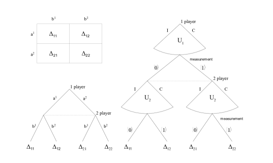
Figure 1: Static game (a), its equivalent in the extensive form (b) and the quantum realization of these game (c). In the quantum realization each of players chooses among continuum of actions specifying $\phi$ i $\theta$. The range of possibilities corresponds to two edges $J$ i $C$ connected with an arc.

The game $\mathrm{Q}\Gamma_{1}$ is depicted in the right-hand side of Figure 1. Game $(N,C(\mathcal{H}),\widetilde{P},\widetilde{u})$ generated by $\mathrm{Q}\Gamma_{1}$ and game (22) are isomorphic via a bijective map $\xi\colon H\to C(\mathcal{H})$ presented as:

$$\xi(h)=\left\{\begin{array}[]{lll}\emptyset,&\mbox{if}&h=\emptyset;\\ q_{1}|[(\nu_{1})],&\mbox{if}&h=(a_{\nu_{1}});\\ (q_{1},q_{2})|[(\nu_{1},\nu_{2})],&\mbox{if}&h=(a_{\nu_{1}},b_{\nu_{1}}).\end{array}\right.$$ (24)

According to Definition 4.3 game $\mathrm{Q}\Gamma_{1}$ is a quantum realization of game $\Gamma_{1}$. Let find out course of the game for an arbitrary strategy profile $s=(s_{1},s_{2})$ and then an outcome corresponds to $s$.

Each of the players have only one information set, respectively, $\mathcal{J}_{1}=\{\emptyset\}$ and $\mathcal{J}_{2}=\{[(0_{1})],[(1_{1})]\}$. It implies that profile $(s_{1},s_{2})$ is tantamount with action profile $(U_{1},U_{2})$ where $U_{j}\in\mathcal{U}_{j}$. As the components of $\mathrm{Q}\Gamma_{1}$ dictate, the game starts with unitary operation $U_{1}$ that player 1 acts on a first qubit of initial state $|\Psi\rangle$:

$$|\Psi_{U_{1}}\rangle = \cos\frac{\gamma}{2}\Biggl{(}e^{i\phi_{1}}\cos\frac{\theta_{1}}{2}|0\rangle-\sin\frac{\theta_{1}}{2}|1\rangle\Biggr{)}\otimes|0\rangle$$ (25)

$$+ \sin\frac{\gamma}{2}\Biggl{(}\sin\frac{\theta_{1}}{2}|0\rangle+e^{-i\phi_{1}}\cos\frac{\theta_{1}}{2}|1\rangle\Biggr{)}\otimes|1\rangle.$$

Then a measurement on this qubit is preparing. If $M_{0_{1}}=|0\rangle\langle 0|\otimes I$ then the probability of obtaining on the first qubit the outcome $0_{1}$ and the state $|\Psi_{U_{1}}\rangle$ after the measurement are:

$$\Pr(0_{1}) = \cos^{2}\frac{\gamma}{2}\cos^{2}\frac{\theta_{1}}{2}+\sin^{2}\frac{\gamma}{2}\sin^{2}\frac{\theta_{1}}{2},$$

$$|\Psi_{\{U_{1},0_{1}\}}\rangle = \frac{1}{\sqrt{\Pr(0_{1})}}\Biggl{(}e^{i\phi_{1}}\cos\frac{\gamma}{2}\cos\frac{\theta_{1}}{2}|00\rangle+i\sin\frac{\gamma}{2}\sin\frac{\theta_{1}}{2}|01\rangle\Biggr{)}.$$ (26)

An analogous calculation for $M_{1_{1}}=|1\rangle\langle 1|\otimes I$ give:

$$\Pr(1_{1}) = \cos^{2}\frac{\gamma}{2}\sin^{2}\frac{\theta_{1}}{2}+\sin^{2}\frac{\gamma}{2}\cos^{2}\frac{\theta_{1}}{2},$$

$$|\Psi_{\{U_{1},1_{1}\}}\rangle = \frac{1}{\sqrt{\Pr(1_{1})}}\Biggl{(}-\cos\frac{\gamma}{2}\sin\frac{\theta_{1}}{2}|10\rangle+ie^{-i\phi_{1}}\sin\frac{\gamma}{2}\cos\frac{\theta_{1}}{2}|11\rangle\Biggr{)}.$$ (27)

After each of histories $\{U_{1},0_{1}\}$ and $\{U_{1},1_{1}\}$ it is the player 2 turn now. All histories after which the second player make move, belong to her information set. It follows that, she performs an operation $U_{2}$ on the second qubit regardless of a measurement outcome on the first qubit. If a couple $\{U_{1},0_{1}\}$ occurred, the state becomes:

$$|\Psi_{\{U_{1},0_{1}\},U_{2}}\rangle = \frac{1}{\sqrt{\Pr(0_{1})}}\Biggl{(}e^{i\phi_{1}}\cos\frac{\gamma}{2}\cos\frac{\theta_{1}}{2}|0\rangle\otimes\biggl{(}e^{i\phi_{2}}\cos\frac{\theta_{2}}{2}|0\rangle-\sin\frac{\theta_{2}}{2}|1\rangle\biggr{)}$$ (28)

$$+ i\sin\frac{\gamma}{2}\sin\frac{\theta_{1}}{2}|0\rangle\otimes\biggl{(}\sin\frac{\theta_{2}}{2}|0\rangle+e^{-i\phi_{2}}\cos\frac{\theta_{2}}{2}|1\rangle\biggr{)}\Biggr{)}.$$

By use of equations (7) expression (28) can be rewritten in the form:

$$|\Psi_{\{U_{1},0_{1}\},U_{2}}\rangle=\frac{\chi_{00}|00\rangle+\chi_{01}|01\rangle}{\sqrt{\Pr(0_{1})}}.$$ (29)

The probability of getting outcome $\nu_{2}\in\{0,1\}$ and the post-measurement state given that outcome $\nu_{2}$ occurred are

$$\Pr(\nu_{2})=\frac{|\chi_{0\nu_{2}}|^{2}}{\Pr(0_{1})},\quad|\Psi_{\{U_{1},0_{1}\},\{U_{2},\nu_{2}\}}\rangle=\frac{\chi_{0\nu_{2}}|0\nu_{2}\rangle}{\sqrt{\Pr(0_{1})}}.$$ (30)

In case if history $\{U_{1},1_{1}\}$ has occurred we get

$$\Pr(\nu_{2})=\frac{|\chi_{1\nu_{2}}|^{2}}{\Pr(1_{1})},\quad|\Psi_{\{U_{1},1_{1}\},\{U_{2},\nu_{2}\}}\rangle=\frac{\chi_{1\nu_{2}}|1\nu_{2}\rangle}{\sqrt{\Pr(1_{1})}}.$$ (31)

Let determine a payoff vector correspond to $U=(U_{1},U_{2})$. Notice first that a set of all terminal histories consistent with $(U_{1},U_{2})$ is made up of four histories at most. The form of this set is

$$\{(q_{1},q_{2})|U\}=\bigl{\{}(\{U_{1},\nu_{1}\},\{U_{2},\nu_{2}\})\colon(\nu_{1},\nu_{2})\in\{0,1\}^{2}\bigr{\}}.$$ (32)

The probability distribution $\Pr(\cdot)$ on the set (32) are expressed by the formula $\Pr(\{U_{1},\nu_{1}\},\{U_{2},\nu_{2}\})=|\chi_{\nu_{1}\nu_{2}}|^{2}$ through (25) to (31) and the utility function $\widetilde{u}$ defined on the same domain takes values $\widetilde{u}(\{U_{1},\nu_{1}\},\{U_{2},\nu_{2}\})=\Delta_{\nu_{1}\nu_{2}}$. Substituting the last calculations to the formula (21) the expected payoffs for the players is as follows$\colon$

$$\widetilde{u}(U)=\sum_{(\nu_{1},\nu_{2})\in\{0,1\}^{2}}|\chi_{\nu_{1}\nu_{2}}|^{2}\Delta_{\nu_{1}\nu_{2}}.$$ (33)

The utility payoffs assigned to $(U_{1},U_{2})$ are the same as the one in Eisert’s et al scheme.

Example 5.2

Let us consider a three player extensive game given in Figure 2$\colon$

$$\Gamma_{2}=(\{1,2,3\},H,P,(I_{i})_{i\in\{1,2,3\}},u)$$ (34)

determined by the following components:

1. $H=\{\emptyset,(a_{0}),(a_{1}),(a_{0},c_{0}),(a_{0},c_{1}),(a_{1},b_{0}),(a_{1},b_{1}),(a_{1},b_{0},c_{0}),(a_{1},b_{0},c_{1})\}$,

2. $P(\emptyset)=1,~{}P(a_{1})=2,~{}P(a_{0})=P(a_{1},b_{0})=3$,

3. $I_{1}=\{\emptyset\},~{}I_{2}=\{(a_{1})\},~{}I_{3}=\{(a_{0}),(a_{1},b_{0})\}$,

4. $u(a_{0},c_{0})=(3,3,1)$, $u(a_{0},c_{1})=(0,0,0)$, $u(a_{1},b_{1})=(2,2,2)$, $u(a_{1},b_{0},c_{0})=(5,5,0)$, $u(a_{1},b_{0},c_{1})=(0,0,1)$.

Figure 2: The modified Selten’s Horse game defined by $\Gamma_{2}$

It is a modified Selten’s Horse game towards the payoffs. Profiles$\colon$ $(a_{0},b_{1},c_{0})$ and $(a_{1},b_{1},c_{1})$ are Nash equilibria in this game and each of them could be equally likely as a scenario of the game indeed. The payoff for players 1 i 2 assigned to $(a_{0},b_{1},c_{0})$ is more beneficial than the outcome corresponding to $(a_{1},b_{1},c_{1})$ that is desirable for player 3. The uncertainty of a result of the game follows from the peculiar strategic position of player 3. She could try to affect decision the others through her announcement before the game starts that she is going to put action $c_{1}$. Then, under the preference of the others players the history $(a_{1},b_{1})$ should occur given that the statement of player 3 is credible enough.

There are games among the quantum realizations of game $\Gamma_{2}$ that have unique Nash equilibrium and that profile would be treated as reasonable profile for players. One of these games is shown below.

$$Q\Gamma_{2}=(\{1,2,3\},|\Psi\rangle,\{\mathcal{U}_{1},\mathcal{U}_{2},\mathcal{U}_{3}\},\mathcal{H},\widetilde{P},\widetilde{u})$$ (35)

with initial state:

$$|\Psi\rangle=\cos\frac{\gamma}{2}|000\rangle+i\sin\frac{\gamma}{2}|111\rangle,\quad\rm{dla}\quad\gamma\in(0,\pi)$$ (36)

and the other components:

1. $\mathcal{U}_{j}=\{V_{0},V_{1}\}$ are defined by formula (12),

2. $\mathcal{H}=\{\emptyset,[(0_{1})],[(1_{1})],[(0_{1},0_{3})],[(0_{1},1_{3})],[(1_{1},0_{2})],[(1_{1},1_{2})],[(1_{1},0_{2},0_{3})],[(1_{1},0_{2},1_{3})]\}$,

3. $\widetilde{P}(\emptyset)=1$, $\widetilde{P}([(1_{1})])=\{2\}$, $\widetilde{P}([(0_{1})])=\widetilde{P}([(1_{1},0_{2})])=\{3\}$,

4. $\widetilde{u}([(1_{1},0_{2},0_{3})])=\{(5,5,0)\}$, $\widetilde{u}([(1_{1},0_{2},1_{3})])=\{(0,0,1)\}$, $\widetilde{u}([(1_{1},1_{2}])=\{(2,2,2)\}$, $\widetilde{u}([(0_{1},0_{3})])=\{(3,3,1)\}$, $\widetilde{u}([(0_{1},1_{3})])=\{(0,0,0)\}$.

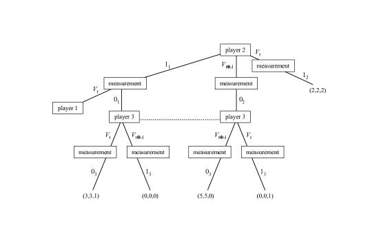
Figure 3: Quantum realization of $\mathrm{Q}\Gamma_{2}$. The graph represents the set of all histories that would occur after action chosen by player 1

A convenient representation of this game is shown in Figure 3. Notice first that when player 1 has moved and a couple $\{V_{t},\nu_{1}\}$ has occurred the other players will be only playing in the ‘classical’ game. It follow form a fact that after an action of player 1 (she can only apply an identity and spin-flip operator) and after the measurement the state $\rho$ of the system collapses to one of the form $|\nu_{1}\nu_{2}\nu_{3}\rangle\langle\nu_{1}\nu_{2}\nu_{3}|$. Now, each of the others players acting via $V_{t}$ on her own qubit $j$ can get outcome $0_{j}$ or $1_{j}$ with probability equals 1. Just the same as in games from Example 5.1 here each of the players has a one information set so a set $\{V_{0},V_{1}\}$ is the set of their strategies. We shall focus on analyze which of profiles $V$ of these strategies are Nash equilibria. At first it necessary to determine expected utility value of each possible profile of strategies. As an example we will find the expected payoff for profile $(V_{0},V_{1},V_{0})$. This profile is consistent with two terminal histories: $(\{V_{0},0_{1}\},\{V_{0},0_{3}\})$ and $(\{V_{0},1_{1}\},\{V_{1},0_{2}\},\{V_{0},1_{3}\})$. To see this, notice that strategy $V_{0}$ of player 1 is consistent with history $(\{V_{0},0_{1}\})$ and $(\{V_{0},1_{1}\})$. If history $(\{V_{0},0_{1}\})$ has happened then $\rho_{(\{V_{0},0_{1}\})}=|000\rangle\langle 000|$ and it is player 3’s turn. Her own operation $V_{0}$ from the profile sets the history $(\{V_{0},0_{1}\},\{V_{0},0_{3}\})$. For this reason probability $\Pr(\{V_{0},0_{1}\},\{V_{0},0_{3}\})=\Pr(\{V_{0},0_{1}\})$ and therefore is equal $\cos^{2}\frac{\gamma}{2}$. In a similar way we could confirm that profile $(V_{0},V_{1},V_{0})$ is consistent with terminal history $(\{V_{0},1_{1}\},\{V_{1},0_{2}\},\{V_{0},1_{3}\})$ that occur with probability equal $\sin^{2}\frac{\gamma}{2}$. Finally by formula (21) the expected utilities $\widetilde{u}(V_{0},V_{1},V_{0})$ amount to $(3\cos^{2}\frac{\gamma}{2},3\cos^{2}\frac{\gamma}{2},1)$. If all value $\widetilde{u}(V)$ are at our disposal then by making use of the inequality (1) it turns out that only profiles of the form $V(t)=(V_{t},V_{t},V_{t})$, $t=0,1$ could be (pure) Nash equilibria. Also, it can be concluded from the set of equations below:

$$\left\{\begin{array}[]{l}u_{1}(V(t))-u_{1}(V_{t\oplus_{2}1},V_{t},V_{t})=-2\cos{(t\pi-\gamma)},\\ u_{2}(V(t))-u_{2}(V_{t},V_{t\oplus_{2}1},V_{t})=1-\cos{(t\pi-\gamma)},\\ u_{3}(V(t))-u_{3}(V_{t},V_{t},V_{t\oplus_{2}1})=(1+\cos{(t\pi-\gamma)})/2.\end{array}\right.$$ (37)

that existence of the Nash equilibria depends on the angle $\gamma$. This relation can be represented by:

$$\mathrm{NE}(\gamma)=\left\{\begin{array}[]{lll}V(1),&\mbox{if}&0<\gamma\leqslant\pi/2;\\ V(0),&\mbox{if}&\pi/2\leqslant\gamma<\pi.\end{array}\right.$$ (38)

The expected utilities for the players are $\widetilde{u}_{1}(V(t))=\widetilde{u}_{2}(V(t))=(5+\cos{(t\pi-\gamma)})/2$, $\widetilde{u}_{3}(V(t))=(3-\cos{(t\pi-\gamma)})/2$. It can be see now that each player can gain from playing game $\mathrm{Q}\Gamma_{2}$. Assuming that one of the equilibria will be chosen in $\Gamma_{2}$, players 1 and 2 can assure oneself 2 utility units and player 3 will get 1 unit for sure - all are strictly less than utilities from $\widetilde{u}(V(t))$ irrespective of what a value of $\gamma$ will be. Notice more that there is the unique equilibrium in game $\mathrm{Q}\Gamma_{2}$ if just $\gamma\neq\pi/2$ or in the case $\gamma=\pi/2$ the same utilities are assigned to the both equilibria. It makes the profile $V(t)$ to be considered as reasonable pair of strategies for players to choose in $\mathrm{Q}\Gamma_{2}$.

6 Summary

Our proposal of quantum playing of extensive game constitutes an extension of schemes included in papers [1] and [5] as well as their generalizations shown in [9] and [10] in the way in which extensive games broaden static games. Quantum realization of a static game carry out by means of scheme constructed in third section generates a game whose set of possible outcomes coincides with the scope of outcomes that may be obtained with the use of scheme for describing quantum static games. It is also a natural assumption of a game theory to model of static game in its extensive shape in such a way so that it does not affect the outcome of the game. The main aim of the research was to defined a new scheme and present the concept on meaningful examples. Therefore for clarity of dissertation we restricted to use of concept to only one basic notion applied to analysis of games - notion of Nash equilibrium. In reality it is possible to use a tool in form of an arbitrary equilibrium refinement dedicated to extensive game. Moreover, the two examples that have been given could be substituted with much more complicated dynamic games. The concept of quantum extensive game provides a broad scope of possibilities regarding ways of analyzing these games and above all way of drawing comparisons between a classic game and its quantum equivalent.

References

References

• [1] J. Eisert, M. Wilkens and M. Lewenstein, Quantum Games and Quantum Strategies, Phys. Rev. Lett. 83, 3077-3080 (1999).
• [2] J. Eisert and M.Wilkens, Quantum Games, J. Mod. Opt. 47 2543 (2000).
• [3] P. Fra̧ckiewicz, The Ultimate Solution to the Quantum Battle of the Sexes Game J. Phys. A: Math. Theor. 42 365305 (2009).
• [4] M. Hirvensalo, Quantum Computing, Springer (2004)
• [5] L.Marinatto and T. Weber, A Quantum Approach to Static Games of Complete Information, Phys. Lett. A 272, 291-303 (2000).
• [6] R. B. Myerson Game Theory: Analysis of Conflict, Harvard University Press (1991)
• [7] J. F. Nash, Non-Cooperative Games, Annals of Mathematics 54, 289-295 (1951).
• [8] A. Nawaz and A. H. Toor, Dilemma and Quantum Battle of Sexes J. Phys. A: Math. Gen. 37 4437 (2004).
• [9] A. Nawaz and A. H. Toor, Generalized Quantization Scheme for Two-Person Non-Zero Sum Games, J. Phys. A: Math. Gen. 37 11457-11463 (2004).
• [10] A. Nawaz and A.H. Toor, The Role of Measurement in Quantum Games, J. Phys. A: Math. Gen. 39 2791-2795 (2006).
• [11] M. A. Nielsen and I. L. Chuang, Quantum Computation and Quantum Information, Cambridge University Press, (2000).
• [12] M. J. Osborne and A. Rubinstein, A Course in Game Theory, MIT Press (1994).