A differential algorithm for the Lyapunov spectrum

Abstract

We present a new algorithm for computing the Lyapunov exponents spectrum based on a matrix differential equation. The approach belongs to the so called continuous type, where the rate of expansion of perturbations is obtained for all times, and the exponents are reached as the limit at infinity. It does not involve exponentially divergent quantities so there is no need of rescaling or realigning of the solution. We show the algorithm’s advantages and drawbacks using mainly the example of a particle moving between two contracting walls.

I Introduction

Lyapunov characteristic exponents (LCE) measure the rate of exponential divergence between neighbouring trajectories in the phase space. The standard method of calculation of LCE for dynamical systems is based on the variational equations of the system. However, solving these equations is very difficult or impossible so the determination of LCE also needs to be carried out numerically rather than analytically.

The most popular methods which are used as an effective numerical tool to calculate the Lyapunov spectrum for smooth systems relies on periodic Gram-Schmidt orthonormalisation of Lyapunov vectors (solutions of the variational equation) to avoid misalignment of all the vectors along the direction of maximal expansion (Galgani , Christansen ).

In some approaches, usually involving a new differential equation instead of the variational one, the procedure of re-orthonormalisation is not used Ranga – these are usually called the continuous methods. They are usually found to be slower than the standard ones due to the underlying equation being more complex than the variational one. A comparison of various methods with and without orthogonalisation can be found in Rama ; Geist and a recent general review in Skokos .

The main goal of this paper is to present a new algorithm for obtaining the LCE spectrum without the rescaling and realigning. This application is a consequence of the equation satisfied by the Lyapunov matrix or operator (see below) which was discovered in one of the authors’ PhD thesis PhD . The particular numerical technique introduced here is the first attempt and is open to further development so it still bears the disadvantages of the usual continuous methods. However, in our opinion, the main advantages of the approach lie in its founding equations and are as follows:

• The whole description of the LCE is embedded in differential geometry from the very beginning, so that and it is straightforward to assign any metric to the phase space including one with non-trivial curvature.

• As the rate of growth is described by an operator (endomorphism) on the tangents space, and the equation it satisfies is readily expressed with the absolute derivative, the approach is explicitly covariant. (The exponents are obviously invariants then, although their transformation properties still seem to be a live issue, see e.g. Eich .)

• There is no need for rescaling and realignment, as the main matrix is at most linear with time, and encodes the full spectrum of LCE.

• Since we make no assumptions on the eigenvalues, there are no problems with the degenerate case encountered in some other methods.

• We rely on a single coordinate-free matrix equation, which reduces the method’s overall complexity.

• The fundamental equation is not an approximation but rather the differential equation satisfied by the so-called time-dependent Lyapunov exponents. This opens potential way to analytic studies of the exponents.

It should be noted that the last points imply a hidden cost (in the current implementation) of diagonalising instead of reorthonormalising, due to the complex matrix functions involved. Fortunately, this procedure needs to be carried out on symmetric matrices for which it is stable.

The natural domain of application of this method might be the General Relativity and dynamical systems of cosmological origin – already formulated in differential geometric language Xin ; Szyd1 ; Szyd2 . Of course this still requires the resolution of the question of the time parameter, and natural metric in the whole phase space (not just the configuration space which corresponds to the physical space-time). Regardless of that choice, however, the fundamental equation of our method will remain the same – whether one chooses to consider the proper interval as the time parameter, or find some external time for an eight dimensional phase space associated to the four dimensional space-time. This stems from the fact that our approach works on any manifold.

Here, we wish to focus on the numerical aspect of the method, providing the rough first estimates of its effectiveness. This is a natural question, after the theoretical motivation for a given method has been established, namely how well it performs numerically. There are obviously many ways of translating the method into code, and we hope for future improvements, nevertheless, the presented implementation can be considered a complete, ready-to-use tool. In the next sections we review the derivation of the main equation and then proceed to the simple mechanical examples for testing and results.

II The base system of equations

For a given system of $n$ ordinary differential equations

$$\dot{x}=f(x,t),\;\;x\in\mathbb{R}^{n},$$ (1)

the variational equations along a particular solution $\varphi(t)$ are defined as

$$\dot{Z}=AZ,\;A:=\left.\frac{\partial f}{\partial x}\right|_{x=\varphi(t)},$$ (2)

and the largest Lyapunov exponent can be defined as

$$\lambda_{\mathrm{m}ax}=\lim_{t\rightarrow\infty}\frac{\ln(\|Z\|)}{t},$$ (3)

for almost all initial conditions of $Z$. From now on we take the norm to be

$$\|Z\|:=\sqrt{Z^{T}Z},$$ (4)

where $Z$ is treated as a column vector, and $T$ denotes transposition. That is to say the metric in the tangent space is Euclidean, as is usually assumed for a given physical systems. This needs not be the case, and a fully covariant derivation of the main equation can be found in PhD .

The above definitions are intuitively based on the fact that for a constant $A$, the solution of (2) is of the form

$$Z=\exp(At)Z(0),$$ (5)

and $\lambda_{\mathrm{max}}$ is the greatest real part of the eigenvalues of $A$. In the simplest case of a symmetric $A$, the largest exponent is exactly the largest eigenvalue. To extend this to the whole spectrum, we note that any solution of (2) is given in terms of the fundamental matrix $F$ so that

$$Z=FZ(0),\;\;\dot{F}=AF,\;\;F(0)=\mathbf{1}.$$ (6)

Then (if the limit exists), the exponents are

$$\{\lambda_{1},\ldots,\lambda_{n}\}=\mathrm{spec}\left(\lim_{t\rightarrow\infty}\frac{\ln(F^{T}F)}{2t}\right).$$ (7)

Since $F^{T}F$ is a symmetric matrix with non-negative eigenvalues, the logarithm is well defined. The additional factor of 2 in the denominator results from the square root in the definition of the norm above.

As we expect $F$ to diverge exponentially, there is no point in integrating the variational equation in itself, but rather to look at the logarithm. To this end we introduce the two matrices $M$ and $L$:

$$M:=FF^{T}=F(F^{T}F)F^{-1}=:\exp(2L).$$ (8)

Clearly $M$ has the same eigenvalues as $F^{T}F$ to which it is connected by a similarity transformation, and the eigenvalues of $L$ behave as $t\lambda$ for large times

$$\{\lambda_{1},\ldots,\lambda_{n}\}=\mathrm{spec}\left(\lim_{t\rightarrow\infty}\frac{L}{t}\right).$$ (9)

That is why we call $L$ the Lyapunov matrix.

To derive the differential equation satisfied by $L$ we start with the derivative of $M$ and use the property of the matrix (operator) exponential

$$\dot{M}=AFF^{T}+FF^{T}A^{T} =e^{2L}\int_{0}^{1}e^{-2aL}2\dot{L}e^{2aL}\mathrm{d}a$$ (10)

$$e^{-2L}Ae^{2L}+A^{T} =2\int_{0}^{1}e^{-2a[L}\dot{L}\mathrm{d}a,$$

where we have introduced a concise notation for the the adjoint of $L$ acting on any matrix $X$ as

$$[L(X)=[L,X],$$ (11)

and used its property

$$e^{-L}Xe^{L}=e^{-[L}X.$$ (12)

Next, the integral is evaluated taking the integrand as a formal power series in $[L$

$$e^{-2[L}A+A^{T}=2\frac{e^{-2[L}-\mathbf{1}}{-2[L}\dot{L},$$ (13)

where the fraction is understood as a power series also, so that there are in fact no negative powers of $[L$. Alternatively one could justify the above by stating that the function

$$\psi_{1}(u)=\frac{1-e^{-2u}}{u}$$ (14)

is well behaved on the spectrum of $[L$ which is contained in $\mathbb{R}$. As $\psi_{1}$ is never zero for a real argument, we can invert the operator on the left-hand side of (13) to get

$$\frac{[L}{1-e^{-2[L}}\left(e^{-2[L}(\theta+\omega)+\theta-\omega\right)=\dot{L},$$ (15)

where the symmetric and antisymmetric parts of $A$ are

$$\theta=\frac{1}{2}(A+A^{T}),\;\;\omega=\frac{1}{2}(A^{T}-A^{T}).$$ (16)

This allows for the final simplification to

$$\dot{L}=[L\coth\left([L\right)\theta-[L,\omega]$$ (17)

The function $\psi_{2}(u)=u\coth(u)$ should be understood as the appropriate limit at $u=0$, so that it is well behaved for all real arguments. As was proven in PhD , the above equation is essentially the same in general coordinates:

$$\nabla_{v}L=\psi_{2}([L)\theta-[L,\omega],$$ (18)

where $v$ is the vector field associated with (1), and $\nabla$ is the covariant derivative.

Note that in this form it is especially easy to obtain the known result for the sum of the exponents. Since trace of any commutator is zero, the only term left is the “constant” term of $\psi_{2}$ which is 1 (or rather the identity operator) so that

$$\frac{\mathrm{d}}{\mathrm{d}t}\sum_{i=1}^{n}t\lambda_{i}=\frac{\dot{V}}{V}=\mathrm{tr}\,\theta,$$ (19)

where $V$ is the volume of the parallelopiped formed by $n$ independent variation vectors.

Another simple consequence occurs when the $\theta$ matrix is zero, the whole equation becomes a Lax equation

$$\dot{L}=[\omega,L],$$ (20)

which preserves the spectrum over time, so that $L/t$ tends to zero at infinity. Another way of looking at it is that it is a linear equation in $L$ and the matrix of coefficients $[\omega$ is antisymmetric in the adjoint representation, so that the evolution is orthogonal and the matrix norm (Frobenius norm to be exact) of $L$ is constant which means $L/t$ tends to the zero matrix. The simplest example of this is the harmonic oscillator or any critical point of the centre type. The variations are then vectors of constant length and the evolution becomes a pure rotation. The authors are not aware of any complex or non-linear system that would exhibit such simple behaviour. Already for the mathematical pendulum such picture is achieved only asymptotically for solutions around its stable critical point. One could expect that a system with identically zero exponents might not be “interesting” enough to incur this kind of research.

We have thus arrived at a dynamical system determining $L$, with right-hand side being given as operations of the adjoint of $L$ on time dependent (through the particular solution) matrices $\theta$ and $\omega$. The next section deals with the practical application of the above equation.

III Exemplary implementation

The main difficulty in using (17) is the evaluation of the function of the adjoint operator. Since we will be integrating the equation to obtain the elements of the matrix $L$, it would be best to have the right-hand side as an explicit expression in those elements. This can be done for the $n=2$ case, but already for $n=3$ one has dozens of terms on the right, and for higher dimensions the number of terms is simply too large for such an approach to be of practical value. An alternative (although equivalent) dynamical system formulation for the mentioned low dimensionalities have been studied in Ranga , but again the complexity of the equations increases so fast with the dimension that the practical value is questionable. Our method, on the other hand, can be made to rely on the same equation for all dimensions, and the only complexity encountered will be the diagonalisation of a symmetric matrix of increasing size.

Another problem lies in the properties of the $\psi_{2}(u)$ function which, although finite for real arguments, has poles at $u=\pm i\pi$. This means that a series approximation is useless, as it would converge only for eigenvalues smaller than $\pi$ in absolute value, whereas we expect them to grow linearly with time and need the results for $t\rightarrow\infty$. On the other hand, $\psi_{2}(u)\rightarrow|u|$ for large $u$ but, unfortunately, the adjoint operator always has $n$ eigenvalues equal to zero, and for Hamiltonian systems it is also expected that two eigenvalues tend to zero.

Thus, as we require the knowledge of $\psi_{2}$ for virtually any symmetric matrix $L$, and we are going to integrate the equation numerically anyway, we will resort to numerical method for this problem. Because the matrix $L$ is symmetric (Hermitian in an appropriate setting) so is its adjoint $[L$, and the best numerical procedure to evaluate its functions is by direct diagonalisation Higham . Obviously this is the main disadvantage of the implementation method as even for symmetric matrices, finding the eigenvalues and all the eigenvectors is time-consuming. So far the authors have only been able to find one alternative routine which is to numerically integrate not $L$ itself but rather the diagonal matrix of its eigenvalues and the accompanying transformation matrix of eigenvectors. However, due to the increased number of matrix multiplications the latter method does not seem any faster than the former.

With this in mind, let us see how the diagonal form of $L$ simplifies the equation. First, we need to regard $[L$ as an operator, and since it is acting on matrices we will adopt a representation where any $n\times n$ matrix becomes a $n^{2}\times 1$ matrix, i.e. a $n^{2}$ element vector constructed by writing all the elements of successive rows as one column. $[L$ is then a $n^{2}\times n^{2}$ matrix. Fortunately, one does not need to diagonalise $[L$ but only $L$ itself. As can be found by direct calculation, the eigenvalues of the adjoin are all the differences of the eigenvalues of $L$. For example

$$L_{D}=\left(\begin{matrix}L_{1}&0\\ 0&L_{2}\end{matrix}\right)\;\Rightarrow\;[L_{D}=\left(\begin{matrix}0&0&0&0\\ 0&L_{1}-L_{2}&0&0\\ 0&0&L_{2}-L_{1}&0\\ 0&0&0&0\end{matrix}\right),$$ (21)

where the subscript $D$ denotes “diagonal”.

Now let us assume we also have the transformation matrix such that

$$L=QL_{D}Q^{T}.$$ (22)

Then, instead of bringing the whole equation to the eigenbasis of $L$, one can only deal with the $\theta$ matrix in the following way

$$\psi_{2}([L)\theta=Q\,\psi_{2}([L_{D})Q^{T}\theta=Q\,\psi_{2}([L_{D})\widetilde{\theta}\,Q^{T},\;\;\widetilde{\theta}:=Q^{T}\theta\,Q.$$ (23)

Of course, the other term of equation (17) can be evaluated as the standard commutator. For the above example the $\psi_{2}$ part would be

$$\psi_{2}([L_{D})=\left(\begin{matrix}1&0&0&0\\ 0&\psi_{2}(L_{1}-L_{2})&0&0\\ 0&0&1&0\\ 0&0&0&\psi_{2}(L_{2}-L_{1})\end{matrix}\right),$$ (24)

and converting $\widetilde{\theta}$ to a vector we get

$$\psi_{2}([L_{D})\tilde{\theta}=\psi_{2}([L_{D})\begin{pmatrix}\tilde{\theta}_{11}&\tilde{\theta}_{12}\\ \tilde{\theta}_{21}&\tilde{\theta}_{22}\end{pmatrix}=\psi_{2}([L_{D})\begin{pmatrix}\tilde{\theta}_{11}\\ \tilde{\theta}_{12}\\ \tilde{\theta}_{21}\\ \tilde{\theta}_{22}\end{pmatrix}=\begin{pmatrix}\tilde{\theta}_{11}\\ \psi_{2}(\Delta_{12})\tilde{\theta}_{12}\\ \psi_{2}(\Delta_{21})\tilde{\theta}_{21}\\ \tilde{\theta}_{22}\end{pmatrix},$$ (25)

which corresponds to the usual 2 by 2 matrix of

$$\psi_{2}([L_{D})\tilde{\theta}=\begin{pmatrix}\tilde{\theta}_{11}&\psi_{2}(\Delta_{12})\tilde{\theta}_{12}\\ \psi_{2}(\Delta_{21})\tilde{\theta}_{21}&\tilde{\theta}_{22}\end{pmatrix},$$ (26)

where $\Delta_{ij}:=L_{i}-L_{j}$ are the differences of the eigenvalues of $L$. In general the appropriate ($n\times n$) matrix elements read

$$\left[\psi_{2}([L_{D})\tilde{\theta}\right]_{ij}=\psi_{2}(\Delta_{ij})\tilde{\theta}_{ij},$$ (27)

and this matrix needs to be transformed back to the original basis according to (23) before being used in the main equation.

The matrix elements of $L$ will, in general, grow linearly with time. This is of course a huge reduction when compared with the exponential growth of the perturbations, but one might want to make them behave even better by taking time into account with

$$L=(t+1)\Lambda.$$ (28)

The reason for the additional 1 is that we will specify the initial conditions at $t=0$ and we want to avoid dividing by zero in the numeric procedure and the limit at infinity (if it exists) is not affected by this change. Of course, in the case of the autonomous systems any value of $t$ can be chosen as initial (at the level of the particular solution) but the non-autonomous case might require a particular value, which can be dealt with in a similar manner.

We now have

$$\dot{\Lambda}=\frac{1}{t+1}\left(\psi_{2}\left((t+1)[\Lambda\right)\theta-\Lambda\right)-[\Lambda,\omega].$$ (29)

As for the initial conditions, the fundamental matrix $F$ is equal to the identity matrix at $t=0$, so that $L(0)=0$ which in turn implies $\Lambda(0)=0$.

We are now ready to state the general steps of the proposed implementation. Choosing a specific numerical routine to obtain the solution for a time step $h$ at each $t$ these are

1. Obtain the particular solution $\varphi(t)$, calculate the Jacobian matrix $A$ at $\varphi$ and, from it, the two matrices $\theta(t)$ and $\omega(t)$. Start with $\Lambda(0)=0$

2. Find the eigenvalues $\lambda_{i}$ and eigenvectors $Q$ of $\Lambda$

3. Transform $\theta(t)$ to $\tilde{\theta}=Q^{T}\theta\,Q$.

4. Compute the auxiliary matrix $\beta_{ij}=[\psi((t+1)[\Lambda_{D})\tilde{\theta}]_{ij}=\psi_{2}((t+1)\Delta_{ij})\tilde{\theta}_{ij}$

5. Take the derivative to be $\dot{\Lambda}(t)=(Q\,\beta\,Q^{T}-\Lambda)/(t+1)-[\Lambda,\omega]$, and use it to integrate the solution to the next step $\Lambda(t+h)$.

6. Repeat steps 2–5 until large enough time is reached.

7. The “time-dependent” Lyapunov exponents at time $t$ are simply $(1+\frac{1}{t})\lambda_{i}$.

The relation in the last point stems from the rescaling (28) and, as can be seen, is only important for small values of $t$.

IV Examples and Comparison

As suggested in the preceding section, one expects this method of obtaining the Lyapunov spectrum to be relatively slow. In order to see that, we decided to compare it with the standard algorithm based on direct integration of the variational equation and Gram-Schmidt rescaling at each step Galgani . Although usually the rescaling is required after times of order 1, we particularly wish to study a system with increasing speed of oscillations and frequent renormalisation will become a necessity. In other words, we want to give the standard method a “head start” when it comes to precision.

For numerical integration we chose the modified midpoint method (with 4 divisions of the whole timestep $H=4h$), which has the advantage of evaluating the derivative fewer times than the standard Runge-Kutta routine with the same accuracy. Since we intended a simple comparison on equal footing, we did not try to optimise either of the algorithms and wrote the whole code in Wolfram’s Mathematica due to the ease of manipulation of the involved quantities and operations (e.g. matrices and outer products).

The most straightforward comparison is for the simplest, i.e. linear dynamical system, for which the main equation (1) is the same as the variational one (2), with constant matrix $A$. The exponents are then known to be the real parts of the eigenvalues of $A$. To include all kinds of behaviour, we took a matrix which has a block form

$$A=\begin{pmatrix}1&-8&0&0\\ 12&1&0&0\\ 0&0&\frac{1}{2}&2\\ 0&0&1&\frac{1}{2}\end{pmatrix},$$ (30)

whose eigenvalues are $\{1+4i\sqrt{6},1-4i\sqrt{6},\frac{1}{2}+\sqrt{2},\frac{1}{2}-\sqrt{2}\}$, so that the LCE are approximately equal to $\{1,1,1.91421,-0.914214\}$.

The basic timestep was taken to be $h=0.01$ and the time to run from 0 to 1000. The results are depicted in figures 1 and 2 with the horizontal axis representing the inverse time $1/t$ so that the sought for limit at infinity becomes the value at zero which is often clearly seen from the trend of the curves. We note that our method required 59 seconds, whereas the standard one only took 17 seconds. The final values of LCE ($t=1000$) were $\{1.00010,0.99990,1.91427,-0.91427\}$ and $\{0.99933,0.99970,1.91372,-0.91372\}$, respectively. The shape of the curves is different, which is to be expected because the matrix $\Lambda$ measures the true growth of the variation vectors at each point of time, and the other method provides more and more accurate approximations to the limit values of the spectrum.

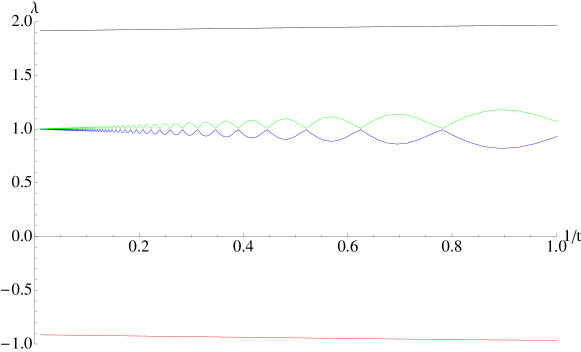
Figure 1: The Lyapunov exponents for the linear system obtained with the presented method.

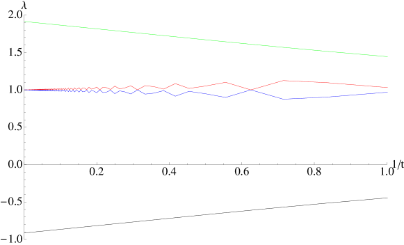
Figure 2: The Lyapunov exponents for the linear system obtained with the standard method.

Before we go on to the central example, which explores a system with accelerating oscillations, we will present numerical results for the system which is synonymous with chaos, namely the Lorenz system Lorenz .

The equations read

$$\dot{x} =\sigma(y-x)$$ (31)

$$\dot{y} =x(\rho-z)-y$$

$$\dot{z} =xy-\beta z,$$

where we took $\sigma=10$, $\beta=8/3$ and $\rho=28$, and integrated the equation for the initial conditions of $x=y=z=10$ from $t=0$ to 1000. Next we integrated the respective methods for the exponents with the timestep of $0.001$. Our method took about 591 seconds and the result is shown in figure 3 with the final value of the spectrum $\{-14.5676,-0.0010078,0.901931\}$. Note that we have shifted the lowest exponent by $+15$, so that all three could be presented on the same plot with enough detail. The standard method took about 152 seconds and its outcome is shown in figure 4 with the final values of $\{-14.5664,0.00173051,0.897989\}$ (we have shifted the graph in the same manner as before).

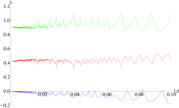
Figure 3: The Lyapunov exponents for the Lorenz system obtained with the new method. The middle exponent has been shifted by +15 to show the details with a better scale.

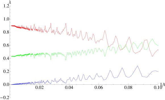
Figure 4: The Lyapunov exponents for the Lorenz system obtained with the standard method. The middle exponent has been shifted by +15 to show the details with a better scale.

One could note that there is less overall variation of the time-dependent exponents in our method similarly to the previous example. A good estimate of precision would be to calculate the sum of the exponents, which, in this system, should be exactly equal to -41/3. The difference between that and the numerical estimates were: for the standard method (at $t=1000$) $-9.04\times 10^{-7}$, and for our method $-9.67\times 10^{-11}$ – a much better result. This seems to be the usual picture for the continuous methods which trade computing time for precision.

A presentation of some more complicated, including both integrable and chaotic, examples can be found in PhD , and for such systems also, we observe the concordance of final results and the speed discrepancy. In order to see how one could benefit from the new method we have to turn to another class of models, ones for which the exponents present oscillatory behaviour. We found that for artificial systems with accelerated oscillations our method performs better and present here a simple physical model which exhibits such property.

Consider a ball moving between two walls which are moving towards each other and assume that the ball bounces off with perfect elasticity. As the distance between the walls decreases and the speed of the ball increases it takes less and less time for each bounce cycle. In order to model this analytically, without resorting to infinite square potential well we will take the following Hamiltonian system

$$H=\frac{1}{2}p^{2}+U\left(\frac{q}{f(t)}\right),\;\;U(x)=\frac{1}{2}\mathrm{artanh}(x)^{2},$$ (32)

which depends on time explicitly via the function $f$ whose meaning is seen as follows: the area hyperbolic tangent is infinite for $x=1$, so that the potential becomes infinite for the position variable $q=f(t)$, so that $f$ is simply half the distance between the walls. In particular we take it to be

$$f(t)=\frac{t+20}{2t+20},$$ (33)

so that it decreases from 1 to $\frac{1}{2}$ slowing down but never stopping. The reason for this is that we want the system not to end in a finite time, and also that the worse behaved $f$ is the faster the numerical integration of the main system itself will fail. The initial shape of the potential and the systems setup is depicted in figure 5

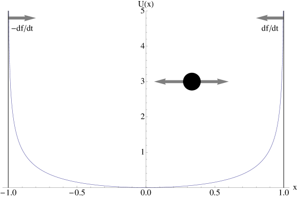
Figure 5: The potential modelling two contracting walls. The vertical lines correspond to the impenetrable barriers of “infinite” $U$. (The vertical position of the ball has no meaning.)

The slowing down of the walls, and the particular shape of $U$ allows us to find rigorous bounds on the Lyapunov exponents. First we note, that the vector tangent to a trajectory in the phase space, i.e. a vector whose components are simply the components of $F$ from (1), is always (for any dynamical system) a solution of the variational equation. That means that just by measuring its length we can estimate the largest exponent, since for almost all initial conditions the resulting evolution is dominated by the largest exponent. Second, the system is Hamiltonian and it must have two exponents of the same magnitude but different signs, so analysing this particular vector will give us all the information regardless of the initial condition. Thus we have to find the following quantity

$$\lambda(t)=\frac{1}{2t}\ln\left(\dot{q}^{2}+\dot{p}^{2}\right)$$ (34)

as a function of time, which boils down to finding bounds on the velocity and acceleration of the bouncing ball.

As the Hamiltonian depends on time explicitly, the energy is not conserved, but instead we have

$$\dot{E}=\frac{\partial H}{\partial t}=U^{\prime}\left(\frac{q}{f}\right)\left(-\frac{q\dot{f}}{f^{2}}\right).$$ (35)

The velocity has its local maxima at $q=0$ when all the energy is in the kinetic term, and we are lead to define a virtual maximal velocity by equating the energy at any given time to a kinetic term

$$\frac{1}{2}v_{M}^{2}:=E,$$ (36)

we will take the positive sign of $v_{M}$, and assume it is non-decreasing as the physical setup suggest. Differentiating the above we get

$$v_{M}\dot{v}_{M}=-U^{\prime}\left(\frac{q}{f}\right)q\frac{\dot{f}}{f^{2}}.$$ (37)

Let us go back to the equation of motion for the momentum variable which reads

$$\dot{p}=-U^{\prime}\left(\frac{q}{f}\right)\frac{1}{f},$$ (38)

and substitute that into the previous equation to get

$$v_{M}\dot{v}_{M}=\dot{p}\,q\frac{\dot{f}}{f}.$$ (39)

As mentioned above $f$ decreases very slowly at late times, which is when we estimate the exponents anyway. We thus assume, that $\dot{f}$ is small enough for the fraction on the right-hand side to be considered constant over one cycle – that is over the time $T$ in which the ball moves from the centre up the potential wall and back to the centre. This time will get shorter and shorter, but also $\dot{f}$ will get closer and closer to zero. The standard problem of the elastic ball and infinitely hard walls shows that the speed transfer at each bounce is of the order of $\dot{f}$ so the (virtual) maximal velocity will change as slowly as $f$ and we are entitled to average the equations over one cycle:

$$v_{M}\dot{v}_{M}=\frac{1}{T}\frac{\dot{f}}{f}\int_{t}^{t+T}\dot{p}\,q\ \mathrm{d}t=\frac{1}{T}\frac{\dot{f}}{f}\left([qp]_{t}^{t+T}-\int_{t}^{t+T}p^{2}\mathrm{d}t\right)\leq-\frac{\dot{f}}{f}v_{M}^{2},$$ (40)

where we integrated by parts and used the fact that at the beginning and end of the cycle $q=0$, and also that the momentum is never greater than the maximal velocity.

We are thus left with a bound in the form of a differential equation, and since all the quantities involved are positive and non-decreasing ($-\dot{f}=|\dot{f}|$), its solution will be the bound for the velocities

$$\dot{q}\leq v_{M}\leq\frac{v_{M0}}{f},$$ (41)

with the “initial” value of $v_{M}$ taken at sufficiently large $t$ so that $\dot{f}$ is small.

Similar considerations can be carried out for the acceleration $\dot{p}$, only this time we have to introduce a virtual points of return $q_{R}$, that is the point at which all the energy is in the potential term

$$U\left(\frac{q_{R}}{f}\right):=E,$$ (42)

since at the real turning points the acceleration reaches its local maxima. Note that this is not the same as $\dot{v}_{M}$ which describes the slow growth of the consecutive maxima of $\dot{q}$ and not the maxima of its slope.

This definition allows us to express $q_{R}$ as a function of $v_{M}$ (via energy)

$$q_{r}=f\tanh(v_{M}),$$ (43)

and the acceleration is

$$\dot{p}\leq a_{M} =\left|-U^{\prime}\left(\frac{q_{R}}{f}\right)\right|=\frac{f\mathrm{artanh}\left(\frac{q_{R}}{f}\right)}{f^{2}-q_{R}^{2}}=\frac{v_{M}}{f(1-\tanh^{2}(v_{M}))}$$ (44)

$$a_{M} =\frac{v_{M0}}{f^{2}}\cosh^{2}\left(\frac{v_{M0}}{f}\right).$$

Bringing the two results together we see that

$$\dot{q}^{2}+\dot{p}^{2}\leq v_{M}^{2}+a_{M}^{2}<\infty,$$ (45)

because the function $f$ does not tend to zero, and by (34) both Lyapunov exponents must in turn be zero themselves. We also recognise that the hyperbolic cosine factor in $a_{M}$ could produce a nonzero exponents if $f$ were to decrease to zero as $1/t$.

Let us now turn to the numerical results of both methods for this system. As initial conditions we take $q(0)=0$ and $p(0)=1$. For the same time step $h=0.01$ we see in figure 6 that the new method predicts the values correctly, integrating for 59 seconds from $t=0$ to $t=1000$. However for the standard one, as shown in figure 7, we see the exponents diverging from zero, for the same time limits, and integrating time of 17 seconds. It turns out $h=0.005$ also gives divergent results and the correct behaviour is recovered for $h=0.001$, shown in figure 8, for which the routine takes 171 seconds.

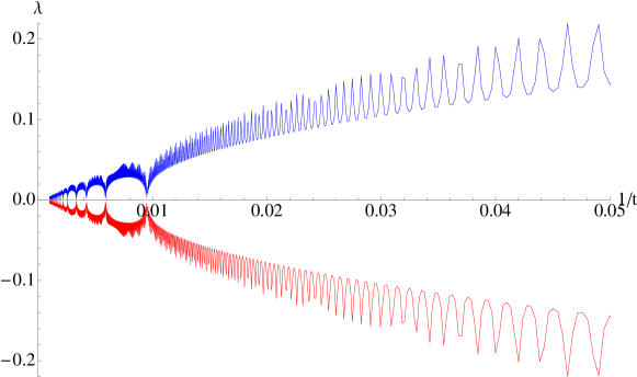
Figure 6: The Lyapunov spectrum obtained with the new method for two contracting walls (timestep $h=0.01$).

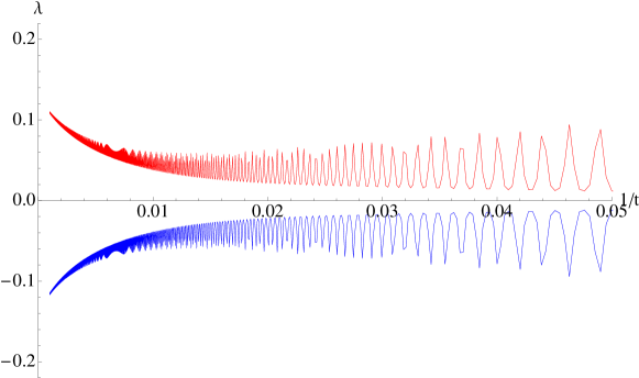
Figure 7: The Lyapunov spectrum obtained with the standard method for two contracting walls (time step $h=0.01$).

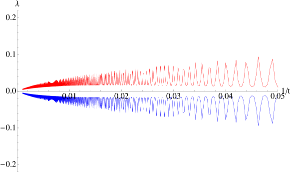
Figure 8: The Lyapunov spectrum obtained with the standard method for two contracting walls (time step $h=0.001$).

V Conclusion

We have presented a new algorithm for evaluation of the Lyapunov spectrum, emerging in the context of differential geometric description of complex dynamical systems. This description seems especially suitable for systems found in General Relativity like, e.g., chaotic geodesic motion smerf . The main advantage of the base method is its covariant nature and concise, albeit explicit, matrix equations that promise more analytic results in the future. Also, this allows for study of curved phase spaces and general dynamical systems – not only autonomous or Hamiltonian ones.

The main differential equation, can be numerically integrated, giving a simple immediate algorithm for the computation of the Lyapunov characteristic exponents. It is in general slower than the standard algorithm (based on Gram-Schmidt orthogonalisation), but the first numerical test suggest it works betters in systems with increasing frequency of (pseudo-)oscillations. We show this on the example of a simple mechanical system – a ball bouncing between two contracting walls.

Although in low dimensions the main equation can be cast into an explicit form (with respect to the unknown variables), in general the numerical integration requires diagonalisation at each step, which is the main disadvantage of the method and the reason of its low speed. We hope to present a more developed algorithm without this problem in the future.

VI Acknowledgements

This paper was supported by grant No. N N202 2126 33 of Ministry of Science and Higher Education of Poland. The authors would also like to thank J. Jurkiewicz and P. Perlikowski for valuable discussion and remarks.

References

- (1) G. Benettin, L. Galgani, A. Giorgilli and J. M. Strelcyn “Lyapunov Characteristic Exponents for smooth dynamical systems and for hamiltonian systems; a method for computing all of them. Part 1: Theory,” Meccanica, 15, 1:9–20 (1980).
- (2) F. Christansen, H. H. Rugh “Computing Lyapunov spectra with continuous Gram - Schmidt orthonormalization”, Nonlinearity 10 1063 (1997).
- (3) Govindan Rangarajan, Salman Habib, Robert D. Ryne, “Lyapunov Exponents without Rescaling and Reorthogonalization”, Phys. Rev. Lett. 80, 17 (1998).
- (4) K. Ramasubramanian and M. S. Sriram, “A comparative study of computation of Lyapunov spectra with different algorithms”, Phys. D 139, 1–2, 72–86 (2000).
- (5) K. Geist, U. Parlitz and W. Lauterborn, “Comparison of different methods for computing Lyapunov exponents”, Prog. Theor. Phys. 83, 875 (1990).
- (6) C. Skokos, “The Lyapunov Characteristic Exponents and their computation”, Lect. Notes Phys. 790, 63-135 (2010)
- (7) Tomasz Stachowiak, “Integrability and Chaos – algebraic and geometric approach”, Doctoral Thesis, Jagiellonian University (2009), arxiv:0810.2968 (math-ph).
- (8) R. Eichhorn, S. J. Linz and P. Hanggi, “Transformation Invariance of Lyapunov Exponents”, Chaos, Solitons and Fractals 12 1377-1383 (2001).
- (9) X. Wu, T. Huang, “Computation of Lyapunov Exponents in General Relativity”, Phys.Lett. A313 77-81 (2003).
- (10) M. Szydlowski, “Toward an invariant measure of chaotic behaviour in general relativity”, Phys. Lett. A 176, 1–2, 22–32 (1993).
- (11) M. Szydlowski and J. Szczesny, “Invariant chaos in Mixmaster cosmology”, Phys. Rev. D50, 819 (1994).
- (12) Functions of Matrices, Nicholas J. Higham, Society for Industrial and Applied Mathematics (2008).
- (13) E. N. Lorenz, “Deterministic nonperiodic flow”, J. Atmos. Sci. 20 (2): 130–141 (1963).
- (14) O. Semerak and P. Sukova, “Free motion around black holeswith discs or rings: between integrability and chaos – I”, Mon. Not. R. Astron. Soc. 404, 545–574 (2010).