Kramers’ formula for chemical reactions in the context of Wasserstein gradient flows

Abstract

We derive Kramers’ formula as singular limit of the Fokker-Planck equation with double-well potential. The convergence proof is based on the Rayleigh principle of the underlying Wasserstein gradient structure and complements a recent result by Peletier, Savaré and Veneroni.

1 Introduction

In 1940 Kramers derived chemical reaction rates from certain limits in a Fokker-Planck equation that describes the probability density of a Brownian particle in an energy landscape [3]. The limit of high activation energy has been revisited in a recent paper by Peletier et al [6], where a spatially inhomogeneous extension of Kramers’ formula is rigorously derived for unimolecular reactions between two chemical states $A$ and $B$. Their derivation relies on passing to the limit in the $L^{2}$-gradient flow structure of the Fokker-Planck equation. It is well-known by now that the Fokker-Planck equation has also an interpretation as a Wasserstein gradient flow [2] and the question was raised in [6] whether Kramers’ formula can also be derived and interpreted within this Wasserstein gradient flow structure. This concept has also been investigated on a formal level for more complicated reaction-diffusion systems in [4]. A further motivation for studying the Fokker-Planck equation within the Wasserstein framework comes from applications that additionally prescribe the time evolution of a moment [1].

In this note we present a rigorous derivation which is based on passing to the limit within the Wasserstein gradient flow structure. To keep things simple we restrict ourselves to the spatially homogeneous case and consider the simplest case of a unimolecular reaction between two chemical states $A$ and $B$, which are represented as two wells of an enthalpy function $H:{\mathbb{R}}\to{\mathbb{R}}$. To avoid unimportant technicalities we assume that the enthalpy function $H$ is a ‘typical’ double-well potential. Specifically, we assume that $H$ is a smooth, nonnegative and even function that satisfies

$$\text{$xH^{\prime}\and{x}<0\;$ for $\;0<\left|{x}\right|<1$},\qquad\text{$xH^{\prime}\and{x}>0\;$ for $\;\left|{x}\right|>1$},$$

with

$$H\and{\pm 1}=H^{\prime}\and{\pm 1}=H^{\prime}\and{0}=0,\quad H\and{0}=H\and{\pm 2}=1,\quad H^{\prime\prime}\and{0}<0<H^{\prime\prime}\and{\pm 1}.$$

The probability density of a molecule with chemical state $x$ is in the following denoted by $\rho$. In Kramers’ approach the molecule performs a Brownian motion in the energy landscape described by $H$, so the evolution of $\rho$ is governed by the Kramers-Smoluchowski equation

$$\partial_{t}\rho=\partial_{x}{\big{(}\partial_{x}\rho+{\varepsilon}^{-2}\rho H^{\prime}\big{)}}\,,$$ (1.1)

where ${\varepsilon}$ is the so-called ’viscosity’ coefficient. In what follows we consider the high activation energy limit ${\varepsilon}^{2}\ll 1$.

The leading order dynamics of (1.1) can be derived by formal asymptotics and governs the evolution of

$$u^{+}(t):=2\int_{0}^{\infty}\rho(t,x)\,dx\,,\qquad u^{-}(t):=2\int_{\infty}^{0}\rho(t,x)\,dx\,,$$

which satisfy $u^{-}\and{t}+u^{+}\and{t}=2$ due to $\int_{\mathbb{R}}{\rho}{\left({t},\,{x}\right)}\,dx=1$. Using WKB methods, for instance, one finds

$$\frac{du^{\pm}}{dt}=\frac{\tau_{\varepsilon}k}{2}\big{(}u^{\mp}-u^{\pm}\big{)},\qquad\tau_{\varepsilon}:={\varepsilon}^{-2}e^{-1/{\varepsilon}^{2}},\qquad k:={\pi}^{-1}\sqrt{|H^{{}^{\prime\prime}}(0)|H^{{}^{\prime\prime}}(1)}.$$ (1.2)

We emphasize that the constant $k$ depends on the details of the function $H$ near its two local minima and its local maximum, and that the time scale is exponentially slow in the height barrier $H(0)/{\varepsilon}^{2}=1/{\varepsilon}^{2}$ between the two wells.

Our goal is to derive (1.2) rigorously by passing to the limit ${\varepsilon}\to 0$ in (1.1). In order to derive a non-trivial limit we have to rescale time accordingly. Thus we consider in the following the probability distribution $\rho_{{\varepsilon}}=\rho_{{\varepsilon}}(t,x)$ that is a solution of

$$\tau_{{\varepsilon}}\partial_{t}\rho_{{\varepsilon}}=\partial_{x}{\big{(}\partial_{x}\rho_{{\varepsilon}}+{\varepsilon}^{-2}\rho_{{\varepsilon}}{H^{\prime}}\big{)}}\,,\qquad x\in\mathbb{R},\;t>0.$$ (1.3)

An important role in the analysis will be played by the unique invariant measure

$$\gamma_{{\varepsilon}}(x):=Z_{{\varepsilon}}^{-1}e^{-H(x)/{\varepsilon}^{2}}\,,\qquad Z_{{\varepsilon}}:=\int_{\mathbb{R}}e^{-H(y)/{\varepsilon}^{2}}\,dy={\varepsilon}\frac{2\sqrt{2\pi}}{\sqrt{H^{{}^{\prime\prime}}(1)}}\big{(}1+o(1)\big{)},$$ (1.4)

which converges in the weak$\star$ topology of probability measures to $\frac{1}{2}(\delta_{-1}+\delta_{+1})$, where $\delta_{\pm 1}$ denotes the delta distributions in $\pm 1$,

As in [6] it is often convenient to switch to the density of $\rho_{{\varepsilon}}$ with respect to $\gamma_{{\varepsilon}}$, that is $u_{{\varepsilon}}=\rho_{{\varepsilon}}/\gamma_{{\varepsilon}}$. Heuristically we expect that $u_{{\varepsilon}}$ is – to leading order in ${\varepsilon}$ – piecewise constant for $x<0$ and $x>0$, where the respective values correspond to $u^{+}$ and $u^{-}$ as introduced above. In what follows we write $u$ instead of $u^{+}$, so $u^{-}$ is given by $2-u$.

For the derivation of the limit equation we assume that our data are well-prepared.

Theorem 1.1

Let $\tau_{{\varepsilon}}$ and $k$ be as in (1.2), and for each ${\varepsilon}$ let $\rho_{{\varepsilon}}:[0,\infty)\times{\mathbb{R}}\to[0,\infty)$ be a solution to (1.1) with initial datum $\rho_{{\varepsilon}}^{0}$. Moreover, suppose that the initial data $\rho_{{\varepsilon}}^{0}$ are probability measures on ${\mathbb{R}}$ that converge weakly$\star$ as ${\varepsilon}\to 0$ to some probability measure $\rho^{0}$, and satisfy

$$\int_{{\mathbb{R}}}\gamma_{{\varepsilon}}|u_{{\varepsilon}}^{0}|^{2}\,dx\,+\,\int_{{\mathbb{R}}}\frac{\gamma_{{\varepsilon}}|\partial_{x}u_{{\varepsilon}}^{0}|^{2}}{\tau_{{\varepsilon}}}\,dx\leq C\,,\qquad u_{{\varepsilon}}^{0}(x)=\rho_{{\varepsilon}}^{0}(x)/\gamma_{{\varepsilon}}(x)\geq c>0\quad\forall\;x\in\mathbb{R}$$

with constants $C$ and $c$ independent of ${\varepsilon}$. Then, for all $t\geq 0$ we have that

$$\rho_{{\varepsilon}}(t,\cdot)\stackrel{{\scriptstyle{\varepsilon}\to 0}}{{\relbar\joinrel\relbar\joinrel\relbar\joinrel\rightharpoonup}}\tfrac{1}{2}\Big{(}u(t)\delta_{+1}+\big{(}2-u(t)\big{)}\delta_{-1}\Big{)}$$

weakly$\star$ in the space of probability measures, where the function $u:[0,\infty)\to[0,\infty)$ satisfies

$$\dot{u}=-k\and{u-1},\qquad\qquad u(0)=u_{0}\,,$$ (1.5)

where $u_{0}=2\int_{0}^{\infty}\rho^{0}\,dx$.

This result has already been derived in [6] in the more general setting with spatial diffusion and under slightly weaker assumptions on the initial data. Our main contribution here is therefore not the result as such, but the method of proof. We answer the question posed in [6], how the passage to the limit can be performed within a Wasserstein gradient flow structure and we identify the corresponding structure for the limit.

We present the formal gradient flow structures of (1.3) as well as (1.5) in section 2. In order to derive the limit equation we pass to the limit in the Rayleigh principle that is associated to any gradient flow. This strategy is inspired by the notion of $\Gamma$-convergence and has already been successfully employed in other singular limits of gradient flows (e.g. in [5]). In section 3 we first obtain some basic a priori estimates as well as an approximation for $u_{{\varepsilon}}$ that will be essential in the identification of the limit gradient flow structure. It is somewhat unsatisfactory that we cannot derive suitable estimates solely from the energy estimates associated to the Wasserstein gradient flow. Instead we use the estimates that correspond to the $L^{2}$-gradient flow structure that is satisfied by $u_{{\varepsilon}}$. It is not obvious to us how this can be avoided.

Section 4 finally contains our main result, that is the novel proof of Theorem 1.1. We show that the limit of $\partial_{t}\rho_{{\varepsilon}}$ satisfies the Rayleigh principle that one obtains as a limit of the Rayleigh principle associated to the Wasserstein gradient structure of (1.3). As a consequence the limit is a solution of (1.5).

2 Gradient flows and Rayleigh principle

We briefly summarize the Wasserstein gradient structure of the Fokker-Planck equation as well as the corresponding gradient flow structure of the limit problem. To point out the key ideas we give a formal exposition and postpone some technical details to Section 3.1.

Given an energy functional $E$ on a manifold ${\cal M}$, whose tangent space $T_{x}{\cal M}$ is endowed with a metric tensor $g_{x}$, the $g$-gradient flow $x(t)$ of $E$ is defined such that

$$g_{x(t)}\big{(}\dot{x}(t),v\big{)}+DE(x(t))v=0$$ (2.6)

for all $v\in T_{x(t)}{\cal M}$ and for all $t>0$. Here $DE(x(t))v$ denotes the directional derivative of $E$ in direction $v$. Our convergence result relies on the Rayleigh principle, that amounts to the observation that a curve $x(t)$ on $\mathcal{M}$ solves (2.6) if and only if for each $t$ the derivative $\dot{x}(t)$ minimizes

$$\tfrac{1}{2}g_{x(t)}\big{(}v,v\big{)}+DE(x(t))v$$

among all $v\in T_{x(t)}{\cal M}$. Slightly more general – and more suitable for generalizations to abstract manifolds in function spaces – is the time integrated version: For each $0<T<\infty$ the function $\dot{x}$ minimizes

$$\int_{0}^{T}\tfrac{1}{2}g_{x(t)}\big{(}v(t),v(t)\big{)}+DE(x(t))v(t)\,dt$$

among all functions $v$ with $v(t)\in T_{x(t)}{\cal M}$ for all $t\in[0,T]$. In what follows we pass to the limit ${\varepsilon}\to 0$ in the time integrated Rayleigh principle because only this one is compatible with the boundedness and compactness results derived below.

To describe the Wasserstein gradient structure of the ${\varepsilon}$–problem (1.3) we consider the formal manifold

$${\cal M}^{{\varepsilon}}:=\Big{\{}\rho_{{\varepsilon}}\colon\mathbb{R}\to[0,\infty)\,,\,\int_{{\mathbb{R}}}\rho_{{\varepsilon}}\,dx=1\Big{\}},\qquad T_{\rho_{{\varepsilon}}}{\cal M}^{{\varepsilon}}:=\Big{\{}v_{{\varepsilon}}\colon\mathbb{R}\to\mathbb{R}\Big{\}}\,,$$

along with the metric tensor

$$g^{{\varepsilon}}_{\rho_{{\varepsilon}}}\big{(}v_{{\varepsilon}},v_{{\varepsilon}}\big{)}:=\tau_{{\varepsilon}}\int_{{\mathbb{R}}}\rho_{{\varepsilon}}|j_{{\varepsilon}}|^{2}\,dx,\qquad\mbox{ where }\quad v_{{\varepsilon}}=-\partial_{x}(\rho_{{\varepsilon}}j_{{\varepsilon}}).$$ (2.7)

The energy of the Fokker-Planck equation is given by

$$E^{{\varepsilon}}(\rho_{{\varepsilon}}):=\int_{{\mathbb{R}}}\rho_{{\varepsilon}}{\big{(}\ln\rho_{{\varepsilon}}+{\varepsilon}^{-2}H\big{)}}\,dx,$$

and has the directional derivative

$$DE^{{\varepsilon}}(\rho_{{\varepsilon}})v_{{\varepsilon}}=\int_{{\mathbb{R}}}v_{{\varepsilon}}\big{(}\ln\rho_{{\varepsilon}}+{\varepsilon}^{-2}H\big{)}\,dx=\int_{{\mathbb{R}}}\rho_{{\varepsilon}}j_{{\varepsilon}}\partial_{x}\big{(}\ln\rho_{{\varepsilon}}+{\varepsilon}^{-2}H\big{)}\,.$$ (2.8)

Consequently, the direction of steepest descent $v_{{\varepsilon}}$ is characterized by the requirement that

$$g^{{\varepsilon}}_{\rho_{{\varepsilon}}}(v_{{\varepsilon}},{\tilde{v}}_{{\varepsilon}})=-DE^{{\varepsilon}}(\rho_{{\varepsilon}}){\tilde{v}}_{{\varepsilon}}\qquad\forall\;{\tilde{v}}_{{\varepsilon}}\in T_{\rho_{{\varepsilon}}}{\cal M}^{{\varepsilon}}.$$

This means

$$j_{{\varepsilon}}=-\tau_{{\varepsilon}}^{-1}\partial_{x}{\big{(}\ln\rho_{{\varepsilon}}+{\varepsilon}^{-2}H\big{)}}\,,$$

and we conclude that (1.3) is in fact the formal $g^{{\varepsilon}}$-gradient flow of $E^{{\varepsilon}}$ on ${\cal M}^{{\varepsilon}}$.

The gradient structure of the limit problem is very simple. The corresponding manifold

$${\cal M}:=\big{\{}u\in(0,2)\big{\}}\,,\qquad T_{u}{\cal M}:=\big{\{}v\in\mathbb{R}\big{\}}$$

is one-dimensional and equipped with the metric tensor

$$g_{u}\big{(}v,v\big{)}:=\frac{v^{2}\,\ln(u/(2-u))}{2k(u-1)}\,.$$

Notice that the metric tensor is continuous in $u$ with $g_{1}{\left({v},\,{v}\right)}=v^{2}/k$, and that $k>0$ is defined in (1.2). The limit energy is given by

$$E(u):=\tfrac{1}{2}\big{(}u\ln u+(2-u)\ln(2-u)\big{)}\,,\qquad DE(u)v=\tfrac{1}{2}\,{v}\ln{\big{(}u/(2-u)\big{)}}\,,$$

and we easily check that (1.5) is the $g$-gradient flow of $E$ on ${\cal M}$.

3 A priori estimates and implications

The density of $\rho_{{\varepsilon}}$ with respect to $\gamma_{{\varepsilon}}$, that is $u_{{\varepsilon}}=\rho_{{\varepsilon}}/\gamma_{{\varepsilon}}$, is smooth and satisfies the equation

$$\tau_{{\varepsilon}}\gamma_{{\varepsilon}}\partial_{t}u_{{\varepsilon}}=\partial_{x}{\big{(}\gamma_{{\varepsilon}}\partial_{x}u_{{\varepsilon}}\big{)}}\,,$$ (3.9)

and hence we readily justify that

$$\int_{{\mathbb{R}}}\gamma_{{\varepsilon}}|u_{{\varepsilon}}|^{2}\,dx\,+\,\frac{2}{\tau_{{\varepsilon}}}\int_{0}^{t}\!\!\!\int_{{\mathbb{R}}}\gamma_{{\varepsilon}}|\partial_{x}u_{{\varepsilon}}|^{2}\,dx\,ds =\int_{{\mathbb{R}}}\gamma_{{\varepsilon}}|u_{{\varepsilon}}^{0}|^{2}\,dx,$$ (3.10)

$$\frac{1}{2\tau_{{\varepsilon}}}\int_{{\mathbb{R}}}\gamma_{{\varepsilon}}|\partial_{x}u_{{\varepsilon}}|^{2}\,dx\,+\,\int_{0}^{t}\!\!\!\int_{{\mathbb{R}}}\frac{|\partial_{t}\rho_{{\varepsilon}}|^{2}}{\gamma_{{\varepsilon}}}\,dx\,ds =\frac{1}{2\tau_{{\varepsilon}}}\int_{{\mathbb{R}}}\gamma_{{\varepsilon}}|\partial_{x}u_{{\varepsilon}}^{0}|^{2}\,dx.$$ (3.11)

Moreover, due to the assumption from Theorem 1.1 the maximum principle for (3.9) implies that

$$\inf\limits_{t\geq{0},\,x\in\mathbb{R},\,{\varepsilon}\geq 0}u_{{\varepsilon}}{\left({t},\,{x}\right)}>0\,.$$ (3.12)

The a priori estimates (3.10) and (3.11) are direct consequences of the $H^{-1}$-gradient and the $L^{2}$-gradient flow structures of (3.9), see [6] for details. The Wasserstein structure, however, implies the a priori estimate

$$\int_{{\mathbb{R}}}\rho_{{\varepsilon}}\and{{\ln\rho_{{\varepsilon}}}+{\varepsilon}^{-2}H}\,dx +\frac{1}{\tau_{{\varepsilon}}}\int_{0}^{t}\!\!\!\int_{{\mathbb{R}}}\rho_{{\varepsilon}}{\big{(}\partial_{x}\and{\ln\rho_{{\varepsilon}}+{\varepsilon}^{-2}H}\big{)}}^{2}\,dxds=\int_{{\mathbb{R}}}\rho_{{\varepsilon}}^{0}\and{\ln\rho_{{\varepsilon}}^{0}+{\varepsilon}^{-2}H}\,dx\,$$

and conserves the mass via $\int_{{\mathbb{R}}}\rho_{{\varepsilon}}\,dx=1$. As mentioned before, our analysis does not make use of this estimate but employs (3.10) and (3.11).

3.1 Rigorous formulation of the Rayleigh principle

We now derive a rigorous setting for the time integrated Rayleigh principle that corresponds to the Wasserstein gradient structure of the Fokker-Planck equation. To this end we suppose that $0<T<\infty$ is fixed and consider the weighted Lebesgue space

$${L^{2}_{\varepsilon}}:=\Big{\{}{f_{\varepsilon}}:[0,T]\times{\mathbb{R}}\to{\mathbb{R}}\;:\;\int_{0}^{T}\int_{\mathbb{R}}\frac{{f_{\varepsilon}}^{2}}{\gamma_{{\varepsilon}}}\,dxdt<0\Big{\}},$$

which is a Hilbert space for each ${\varepsilon}>0$. We also define the linear space

$$\mathcal{T}_{{\varepsilon}}:=\big{\{}\text{$v_{{\varepsilon}}:L^{2}_{{\varepsilon}}$ such that $v_{{\varepsilon}}=-\partial_{x}\and{\rho_{\varepsilon}{j_{\varepsilon}}}$ for some $j_{\varepsilon}$ with $\rho_{\varepsilon}{j_{\varepsilon}}\in{L^{2}_{{\varepsilon}}}$}\big{\}},$$

and show that the Rayleigh principle is a well-posed minimization problem on $\mathcal{T}_{\varepsilon}$.

Lemma 3.1

For each ${f_{\varepsilon}}\in{L^{2}_{\varepsilon}}$ with $\partial_{x}{f_{\varepsilon}}\in{L^{2}_{\varepsilon}}$ we have

$$\int_{0}^{T}\int_{\mathbb{R}}\ln u_{{\varepsilon}}\partial_{x}{f_{\varepsilon}}\,dxdt=-\int_{0}^{T}\int_{\mathbb{R}}\frac{{f_{\varepsilon}}\partial_{x}u_{{\varepsilon}}}{u_{{\varepsilon}}}\,dxdt,$$ (3.13)

and ${f_{\varepsilon}}{\left({\cdot},\,{x}\right)}\to 0$ as $x\to\pm\infty$ strongly in $L^{2}{\big{(}[0,T]\big{)}}$. In particular, we have

$${f_{\varepsilon}}{\left({t},\,{y}\right)}=\int_{\infty}^{y}\partial_{x}{f_{\varepsilon}}{\left({t},\,{x}\right)}\,dx,\qquad\int_{\mathbb{R}}\partial_{x}{f_{\varepsilon}}{\left({t},\,{x}\right)}\,dx=0$$

for almost all ${\left({t},\,{y}\right)}\in[0,T]\times{\mathbb{R}}$.

Proof 3.1.

Clearly, (3.13) holds for all smooth ${f_{\varepsilon}}$ with compact support in $[0,T]\times{\mathbb{R}}$. By approximation in ${L^{2}_{\varepsilon}}$ – and since we have $\gamma_{{\varepsilon}}{\ln u_{{\varepsilon}}},\gamma_{{\varepsilon}}u_{{\varepsilon}}^{-1}\partial_{x}u_{{\varepsilon}}\in{L^{2}_{\varepsilon}}$ due to (3.10), (3.11), (3.12), and $\left|{\ln u_{{\varepsilon}}}\right|\leq{C}\sqrt{u_{{\varepsilon}}}$ – we then conclude that (3.13) holds for all ${f_{\varepsilon}}\in{L^{2}_{\varepsilon}}$. Moreover, using Hölder’s inequality and $\int_{x_{1}}^{x_{2}}\gamma_{{\varepsilon}}\,dx\leq 1$ we find

$$\int_{0}^{T}\big{|}{{f_{\varepsilon}}{\left({t},\,{x_{2}}\right)}-{f_{\varepsilon}}{\left({t},\,{x_{1}}\right)}}\big{|}^{2}\,dt\leq\int_{0}^{T}\left|{\int_{x_{1}}^{x_{2}}{\partial_{x}{f_{\varepsilon}}{\left({t},\,{x}\right)}}\,dx}\right|^{2}\,dt\leq\int_{0}^{T}\int_{x_{1}}^{x_{2}}\frac{\left|{\partial_{x}{f_{\varepsilon}}}\right|^{2}}{\gamma_{{\varepsilon}}}\,dxdt$$

for all $x_{1}<x_{2}$. Therefore, and by assumption on $\partial_{x}{f_{\varepsilon}}$, we know that ${f_{\varepsilon}}{\left({\cdot},\,{x}\right)}$ converges strongly as $x\to\pm\infty$ to some limit functions in $L^{2}{\big{(}[0,T]\big{)}}$. From

$$\int_{0}^{T}\int_{\mathbb{R}}{f_{\varepsilon}}^{2}\,dxdt\leq{{\|{\gamma_{{\varepsilon}}}\|}_{\infty}}\int_{0}^{T}\int_{\mathbb{R}}\frac{{f_{\varepsilon}}^{2}}{\gamma_{{\varepsilon}}}\,dx\,dt<\infty$$

we then infer that these limit functions vanish.

Corollary 2.

We have $\partial_{t}\rho_{{\varepsilon}}\in\mathcal{T}_{\varepsilon}$. Moreover, each $v_{\varepsilon}\in\mathcal{T}_{\varepsilon}$ satisfies $\int_{\mathbb{R}}{v_{\varepsilon}}\,dx=0$ for almost all $t$, as well as

$$\left|{\int_{0}^{T}DE^{{\varepsilon}}(\rho_{{\varepsilon}})v_{{\varepsilon}}\,dt}\right|^{2}\leq\and{\int_{0}^{T}g^{\varepsilon}_{\rho_{{\varepsilon}}}{\left({\partial_{t}\rho_{{\varepsilon}}},\,{\partial_{t}\rho_{{\varepsilon}}}\right)}\,dt}\and{\int_{0}^{T}g^{\varepsilon}_{\rho_{{\varepsilon}}}{\left({v_{\varepsilon}},\,{v_{\varepsilon}}\right)}\,dt}<\infty\,$$ (3.14)

with $g^{\varepsilon}$ and $DE^{\varepsilon}$ as in (2.7) and (2.8).

Proof 3.2.

The first claim follows from $\partial_{t}\rho_{{\varepsilon}}=\partial_{x}\and{\tau_{{\varepsilon}}^{-1}\gamma_{{\varepsilon}}\partial_{x}u_{{\varepsilon}}}$ and since the a priori estimates (3.10) and (3.11) guarantee that $\partial_{t}\rho_{{\varepsilon}}\in{L^{2}_{\varepsilon}}$ as well as $\tau_{{\varepsilon}}^{-1}\gamma_{{\varepsilon}}\partial_{x}u_{{\varepsilon}}\in{L^{2}_{\varepsilon}}$. Now let $v_{{\varepsilon}}=-\partial_{x}f_{\varepsilon}\in\mathcal{T}_{\varepsilon}$ be arbitrary. By definition and (3.12), we have

$$\int_{0}^{T}g^{\varepsilon}_{\rho_{{\varepsilon}}}{\left({v_{\varepsilon}},\,{v_{\varepsilon}}\right)}\,dt=\int_{0}^{T}\int_{\mathbb{R}}\frac{\tau_{{\varepsilon}}\,f_{\varepsilon}^{\,2}}{\rho_{{\varepsilon}}}\,dxdt\leq{C}\int_{0}^{T}\int_{\mathbb{R}}\frac{\tau_{{\varepsilon}}\,f_{\varepsilon}^{\,2}}{\gamma_{{\varepsilon}}}\,dxdt<\infty\,.$$

Moreover, Lemma 3.1 provides $\int_{\mathbb{R}}{v_{\varepsilon}}\,dx=0$ as well as

$$-\int_{0}^{T}DE^{{\varepsilon}}(\rho_{{\varepsilon}})v_{{\varepsilon}}\,dt =\int_{0}^{T}\int_{{\mathbb{R}}}f_{\varepsilon}\partial_{x}\ln u_{{\varepsilon}}\,dxdt=\int_{0}^{T}\int_{\mathbb{R}}\frac{f_{\varepsilon}}{\sqrt{\rho}_{{\varepsilon}}}\frac{\gamma_{{\varepsilon}}\partial_{x}u_{{\varepsilon}}}{\sqrt{\rho}_{{\varepsilon}}}\,dxdt$$

$$\leq\tau_{{\varepsilon}}^{2}\and{\int_{0}^{T}\int_{\mathbb{R}}\frac{f_{\varepsilon}^{\,2}}{\rho_{{\varepsilon}}}\,dxdt}^{1/2}\and{\int_{0}^{T}\int_{\mathbb{R}}\frac{\and{\tau_{{\varepsilon}}^{-1}\gamma_{{\varepsilon}}\partial_{x}u_{{\varepsilon}}}^{2}}{\rho_{{\varepsilon}}}\,dxdt}^{1/2},$$

which is (3.14).

From Corollary 2 we finally conclude that

$$\int_{0}^{T}\tfrac{1}{2}g^{\varepsilon}_{\rho_{\varepsilon}}{\left({v_{{\varepsilon}}},\,{v_{{\varepsilon}}}\right)}+DE^{\varepsilon}(\rho_{{\varepsilon}})v_{{\varepsilon}}\,dt$$ (3.15)

is well defined for $v_{{\varepsilon}}\in\mathcal{T}_{\varepsilon}$, and that $\partial_{t}\rho_{{\varepsilon}}$ is the unique minimizer.

3.2 Compactness result for $\rho_{{\varepsilon}}$

We now exploit the a priori estimates (3.10) and (3.11) to derive suitable compactness results for $\rho_{{\varepsilon}}$, which then allow to extract convergent subsequences. To this end we choose $0<\alpha<1$ independent of ${\varepsilon}$ and define the intervals

$$J^{\pm}_{\varepsilon}:=(\pm 1-{\varepsilon}^{\alpha},\,\pm 1+{\varepsilon}^{\alpha})\,,\qquad J^{0}_{\varepsilon}:=(-{\varepsilon}^{\alpha},\,+{\varepsilon}^{\alpha})\,,\qquad\bar{J}_{\varepsilon}:={\mathbb{R}}\setminus\and{J^{-}_{\varepsilon}{\cup}J^{+}_{\varepsilon}}\,,$$

as well as

$$I^{-}_{\varepsilon}:=(-2+{\varepsilon}^{\alpha},\,-{\varepsilon}^{\alpha})\,,\qquad I^{+}_{\varepsilon}:=({\varepsilon}^{\alpha},\,2-{\varepsilon}^{\alpha})\,,\qquad I_{{\varepsilon}}:=I^{-}_{\varepsilon}\cup{I^{+}_{\varepsilon}}\,.$$

We proceed with summarizing some properties of $\gamma_{{\varepsilon}}$.

Lemma 3.

We have

$$\int_{J^{\pm}_{\varepsilon}}\gamma_{{\varepsilon}}\,dx\quad\xrightarrow{{\varepsilon}\to 0}\quad\frac{1}{2}\,,\qquad\qquad\int_{\bar{J}_{\varepsilon}}\gamma_{{\varepsilon}}\,dx\quad\xrightarrow{{\varepsilon}\to 0}\quad 0\,,$$ (3.16)

as well as

$$\sup\limits_{x\in\bar{J}_{\varepsilon}}\gamma_{{\varepsilon}}\and{x}\quad\xrightarrow{{\varepsilon}\to 0}\quad 0\,,\qquad\qquad\tau_{\varepsilon}^{-1}\inf_{x\in{I_{\varepsilon}}}\gamma_{{\varepsilon}}\and{x}\quad\xrightarrow{{\varepsilon}\to 0}\quad\infty\,,$$ (3.17)

and

$$\int_{J^{0}_{\varepsilon}}\frac{\tau_{{\varepsilon}}}{\gamma_{{\varepsilon}}}\,dx\quad\xrightarrow{{\varepsilon}\to 0}\quad\frac{4}{k}\,,\qquad\qquad\int_{I_{\varepsilon}}\frac{\tau_{{\varepsilon}}}{\gamma_{{\varepsilon}}}\,dx\quad\xrightarrow{{\varepsilon}\to 0}\quad 0\,.$$ (3.18)

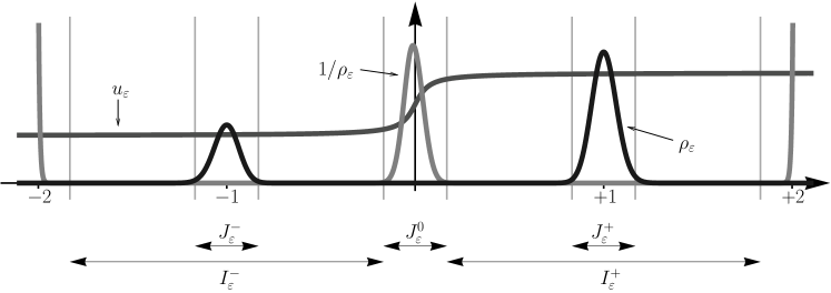
Figure 1: Schematic representation of $\rho_{{\varepsilon}}$, $u_{{\varepsilon}}$, and $1/\rho_{{\varepsilon}}$.

Proof 3.3.

From the definition (1.4) and $\int_{\mathbb{R}}\gamma_{{\varepsilon}}\,dx=1$ we readily derive (3.16). Thanks to our assumptions on $H$ we also have

$$H\and{x}\geq\min{\big{(}H\and{1+{\varepsilon}^{\alpha}},\,H\and{1-{\varepsilon}^{\alpha}}\big{)}}\geq\tfrac{1}{2}\and{1+o(1)}H^{\prime\prime}\and{1}{\varepsilon}^{2\alpha}\qquad\forall\;x\in\bar{J}_{\varepsilon}\,,$$

and this implies (3.17)₁. Similarly, we find

$$H\and{x}\leq\max{\big{(}H\and{{\varepsilon}^{\alpha}},\,H\and{2-{\varepsilon}^{\alpha}}\big{)}}\leq 1+o(1)-\min{\Big{(}\tfrac{1}{2}H^{\prime\prime}\and{0}{\varepsilon}^{2\alpha},\,H^{\prime}\and{2}{\varepsilon}^{\alpha}\Big{)}}\qquad\forall\;x\in{I_{\varepsilon}}$$

and hence (3.17)₂ and (3.18)₂. Finally, a direct computation gives

$$\int_{J^{0}_{\varepsilon}}\frac{\tau_{{\varepsilon}}}{\gamma_{{\varepsilon}}}\,dx =\frac{Z_{{\varepsilon}}}{{\varepsilon}^{2}}\int_{-{\varepsilon}^{\alpha}}^{{\varepsilon}^{\alpha}}\exp\and{-\tfrac{1}{2}H^{\prime\prime}\and{0}{\big{(}1+o(1)\big{)}}x^{2}/{\varepsilon}^{2}}\,dx=\frac{4\pi\,{\big{(}1+o(1)\big{)}}}{\sqrt{H^{{}^{\prime\prime}}(1)|H^{{}^{\prime\prime}}(0)|}}$$

which is (3.18)₁ thanks to (1.2).

Our compactness result for $\rho_{{\varepsilon}}$ is illustrated in Figure 1 and reads as follows.

Lemma 4.

There exists a subsequence ${\varepsilon}\to 0$ along with a function $u\in{H^{1}\and{[0,T]}}$ with weak derivative $\dot{u}$ such that

1. for each $t\in[0,T]$, $\rho_{{\varepsilon}}{\left({t},\,{\cdot}\right)}$ is a probability measure on ${\mathbb{R}}$ that converges weakly$\star$ to $\tfrac{1}{2}{\big{(}u\and{t}\delta_{+1}+\and{1-u(t)}\delta_{-1}\big{)}}$ such that

   $$\int_{J^{\pm}_{\varepsilon}}\rho_{{\varepsilon}}\,dx\quad\xrightarrow{{\varepsilon}\to 0}\quad\tfrac{1}{2}\pm\tfrac{1}{2}\and{u-1}\qquad\text{and}\qquad\int_{\bar{J}_{\varepsilon}}\rho_{{\varepsilon}}\,dx\quad\xrightarrow{{\varepsilon}\to 0}\quad 0\,$$ (3.19)

   uniformly in $t\in[0,T]$,

2. $\partial_{t}\rho_{{\varepsilon}}$ is a measure on $[0,T]\times{\mathbb{R}}$ that converges weakly$\star$ to $\tfrac{1}{2}{\big{(}\dot{u}\delta_{+1}-\dot{u}\delta_{-1}\big{)}}$ such that

   $$\int_{J^{\pm}_{\varepsilon}}\partial_{t}\rho_{{\varepsilon}}\,dx\quad\stackrel{{\scriptstyle{\varepsilon}\to 0}}{{\relbar\joinrel\relbar\joinrel\relbar\joinrel\rightharpoonup}}\quad\pm\tfrac{1}{2}\dot{u}\qquad\text{and}\qquad\int_{\bar{J}_{\varepsilon}}\left|{\partial_{t}\rho_{{\varepsilon}}}\right|\,dx\quad\xrightarrow{{\varepsilon}\to 0}\quad 0$$ (3.20)

   weakly and strongly in $L^{2}{\big{(}[0,T]\big{)}}$, respectively.

Moreover, we have $c\;\leq\;u\and{t},\,2-u\and{t}\;\leq\;2-c$ for some $0<c<2$ and all $t\in[0,T]$.

Proof 3.4.

The estimates (3.10) and (3.11) combined with (3.17) imply

$$\sup_{t\in[0,T]}\and{\int_{\bar{J}_{\varepsilon}}\rho_{{\varepsilon}}\,dx}^{2} \leq\sup_{t\in[0,T]}\and{\int_{{\mathbb{R}}}\gamma_{{\varepsilon}}u_{{\varepsilon}}^{2}\,dx}\and{\int_{\bar{J}_{\varepsilon}}\gamma_{{\varepsilon}}\,dx}\quad\xrightarrow{{\varepsilon}\to 0}\quad 0\,,$$

$$\int_{0}^{T}\and{\int_{\bar{J}_{\varepsilon}}\left|{\partial_{t}\rho_{{\varepsilon}}}\right|dx}^{2}\,dt \leq\int_{0}^{T}\and{\int_{\bar{J}_{\varepsilon}}\gamma_{{\varepsilon}}\left|{\partial_{t}u_{{\varepsilon}}}\right|^{2}\,dx}\and{\int_{\bar{J}_{\varepsilon}}\gamma_{{\varepsilon}}\,dx}\,dt\quad\xrightarrow{{\varepsilon}\to 0}\quad 0\,,$$

and hence we find (3.19)₂ and (3.20)₂. We now consider the functions $u^{\pm}_{\varepsilon}:[0,T]\to{\mathbb{R}}$ defined by

$$\tfrac{1}{2}u^{\pm}_{\varepsilon}\and{t}:=\int_{J^{\pm}_{\varepsilon}}\rho_{{\varepsilon}}{\left({t},\,{x}\right)}\,dx=\int_{J^{\pm}_{\varepsilon}}u_{{\varepsilon}}{\left({t},\,{x}\right)}\gamma_{{\varepsilon}}\and{x}\,dx\,,$$

and using (3.10), (3.11), and (3.17) again we obtain

$$\tfrac{1}{4}{\|{u^{\pm}_{\varepsilon}}\|}^{2}_{L^{2}\and{[0,T]}} \leq\int_{0}^{T}\and{\int_{J^{\pm}_{\varepsilon}}\gamma_{{\varepsilon}}u_{{\varepsilon}}^{2}\,dx}\and{\int_{J^{\pm}_{\varepsilon}}\gamma_{{\varepsilon}}\,dx}\,dt\leq{C}\,,$$

$$\tfrac{1}{4}{\|{\dot{u}^{\pm}_{\varepsilon}}\|}^{2}_{L^{2}\and{[0,T]}} \leq\int_{0}^{T}\and{\int_{J^{\pm}_{\varepsilon}}\gamma_{{\varepsilon}}\left|{\partial_{t}u_{{\varepsilon}}}\right|^{2}\,dx}\and{\int_{J^{\pm}_{\varepsilon}}\gamma_{{\varepsilon}}\,dx}\,dt\leq{C}\,.$$

By weak compactness we can therefore extract a subsequence such that

$$u^{\pm}_{\varepsilon}\;\stackrel{{\scriptstyle{\varepsilon}\to 0}}{{\relbar\joinrel\relbar\joinrel\relbar\joinrel\rightharpoonup}}\;u^{\pm}\quad\text{weakly in $H^{1}{\big{(}[0,T]\big{)}}\subset\subset{C{\big{(}[0,T]\big{)}}}$},\quad$$

for some limit functions $u^{\pm}$. Setting $u:=u_{+}$, the remaining assertions hold either by construction, or thanks to (3.12) and $\int\rho_{{\varepsilon}}\,dx=1$ .

From now on we suppose that a subsequence as in Lemma 4 is chosen and prove the assertions of Theorem 1.1 for this subsequence. Since the function $u$ is uniquely determined by the limit problem (1.5), we then conclude afterwards that Theorem 1.1 holds for all subsequences.

3.3 Leading order description of $u_{{\varepsilon}}$

In order to pass to the limit ${\varepsilon}\to\infty$ in the minimization problem corresponding to (3.15) we show that the relative density $u_{\varepsilon}$ is close to a step function but exhibits a narrow and smooth transition layer at $x=0$ whose shape is determined by $\gamma_{{\varepsilon}}$, see Figure 1. Specifically, we prove that $u_{\varepsilon}$ can be approximated by

$$\tilde{u}_{\varepsilon}{\left({t},\,{x}\right)}:=1+{\big{(}u\and{t}-1\big{)}}\,\eta_{\varepsilon}\and{x}\,,\qquad\eta_{\varepsilon}\and{x}:=\displaystyle 2\int_{0}^{x}\frac{dy}{\gamma_{{\varepsilon}}\and{y}}\;\Big{/}\;\int_{-1}^{1}\frac{dy}{\gamma_{{\varepsilon}}\and{y}}\,.$$ (3.21)

Notice that $\eta_{\varepsilon}$ is an approximation of the sign function on the interval $\left|{x}\right|<2$ because Lemma 3 provides that

$$\sup_{x\in{I_{\varepsilon}}}\left|{\eta_{\varepsilon}\and{x}-\mathrm{sign}\and{x}}\right|\xrightarrow{{\varepsilon}\to 0}0.$$ (3.22)

Lemma 5.

We have

$$\sup_{t\in[0,T],x\in{I^{\pm}_{\varepsilon}}}\big{|}{u_{{\varepsilon}}{\left({t},\,{x}\right)}-\tilde{u}_{\varepsilon}{\left({t},\,{x}\right)}}\big{|}\;\xrightarrow{{\varepsilon}\to 0}\;0\,,\qquad\int_{0}^{T}\sup_{x\in J^{0}_{{\varepsilon}}}\Big{|}u_{{\varepsilon}}(t,x)-\tilde{u}_{\varepsilon}{\left({t},\,{x}\right)}\Big{|}^{2}\,dt\;\xrightarrow{{\varepsilon}\to 0}\;0\,.$$

Proof 3.5.

From (3.11) and (3.17)₂ we infer that

$$\sup_{t\in[0,T]}\int_{I_{\varepsilon}}\left|{\partial_{x}u_{{\varepsilon}}}\right|^{2}\,dx\leq\sup_{t\in[0,T]}\and{\int_{I_{\varepsilon}}\frac{\gamma_{{\varepsilon}}\left|{\partial_{x}u_{{\varepsilon}}}\right|^{2}}{\tau_{{\varepsilon}}}\,dx}\and{\int_{I_{\varepsilon}}\frac{\tau_{{\varepsilon}}}{\gamma_{{\varepsilon}}}\,dx}\xrightarrow{{\varepsilon}\to 0}0\,,$$

and hence $\sup_{t\in[0,T]}\sup_{x,y\in{I^{\pm}_{\varepsilon}}}\big{|}{u_{{\varepsilon}}{\left({t},\,{x}\right)}-u_{{\varepsilon}}{\left({t},\,{y}\right)}}\big{|}\xrightarrow{{\varepsilon}\to 0}0.$ With (3.16) we therefore conclude that

$$\sup\limits_{t\in[0,T]}\sup\limits_{x\in{I^{\pm}_{\varepsilon}}}\left|{u_{{\varepsilon}}{\left({t},\,{x}\right)}-2\int_{J^{\pm}_{\varepsilon}}\rho_{{\varepsilon}}{\left({t},\,{y}\right)}\,dy}\right|\quad\xrightarrow{{\varepsilon}\to 0}\quad 0\,,$$

so Lemma 4 gives

$$\sup\limits_{t\in[0,T]}\sup\limits_{x\in{I^{\pm}_{\varepsilon}}}\big{|}{1\pm\and{u-1}-u_{{\varepsilon}}{\left({t},\,{x}\right)}}\big{|}\quad\xrightarrow{{\varepsilon}\to 0}\quad 0\,.$$

The first assertion now follows from (3.22). Towards the second claim we integrate (3.9) twice with respect to $x$. This gives

$$u_{{\varepsilon}}{\left({t},\,{x}\right)} =\hat{u}_{\varepsilon}{\left({t},\,{x}\right)}+\int_{0}^{x}\frac{\tau_{{\varepsilon}}}{\gamma_{{\varepsilon}}\and{y}}\int_{0}^{y}\partial_{t}\rho_{{\varepsilon}}{\left({t},\,{z}\right)}\,dz\,dy$$ (3.23)

with $\hat{u}_{\varepsilon}{\left({t},\,{x}\right)}:=C_{1,{\varepsilon}}\and{t}\eta_{\varepsilon}\and{x}+C_{2,{\varepsilon}}\and{t},$ where the two constants of integration can be computed by

$$C_{1,{\varepsilon}}\and{t}=\frac{\hat{u}_{\varepsilon}{\left({t},\,{+1/2}\right)}-\hat{u}_{\varepsilon}{\left({t},\,{-1/2}\right)}}{2\eta_{\varepsilon}\and{1/2}},\qquad C_{2,{\varepsilon}}\and{t}=\frac{\hat{u}_{\varepsilon}{\left({t},\,{+1/2}\right)}+\hat{u}_{\varepsilon}{\left({t},\,{-1/2}\right)}}{2}.$$ (3.24)

For $\left|{y}\right|\leq\left|{x}\right|\leq 1-{\varepsilon}^{\alpha}$ the integral term in (3.23) can be estimated by

$$\left|{\int_{0}^{y}\partial_{t}\rho_{{\varepsilon}}{\left({t},\,{z}\right)}\,dz}\right| \leq\Big{(}\int_{0}^{1-{\varepsilon}^{\alpha}}\frac{|\partial_{t}\rho_{{\varepsilon}}{\left({t},\,{z}\right)}|^{2}}{\gamma_{{\varepsilon}}\and{z}}\,dz\Big{)}^{1/2}\Big{(}\int_{0}^{1-{\varepsilon}^{\alpha}}\gamma_{{\varepsilon}}\and{z}\,dz\Big{)}^{1/2}$$

$$\leq C\and{\sup\limits_{\left|{x}\right|\leq{1}-{\varepsilon}^{\alpha}}\gamma_{{\varepsilon}}\and{x}}^{1/2}\and{\int_{{\mathbb{R}}}\frac{|\partial_{t}\rho_{{\varepsilon}}{\left({t},\,{z}\right)}|^{2}}{\gamma_{{\varepsilon}}\and{z}}dz}^{1/2}\,,$$

so (3.11) and Lemma 3 imply

$$\int_{0}^{T}\sup_{\left|{x}\right|\leq{1}-{\varepsilon}^{\alpha}}\Big{|}u_{{\varepsilon}}(t,x)-\hat{u}_{\varepsilon}{\left({t},\,{x}\right)}\Big{|}^{2}\,dt\quad\xrightarrow{{\varepsilon}\to 0}\quad 0\,.$$

In particular, we have $\hat{u}_{\varepsilon}{\left({\cdot},\,{\pm 1/2}\right)}\xrightarrow{{\varepsilon}\to 0}1\pm\and{u-1}$ in $L^{2}{\big{(}[0,T]\big{)}}$. From this, (3.24), and the definition of both $\hat{u}_{\varepsilon}$ and $\tilde{u}_{\varepsilon}$ we finally conclude that

$$\int_{0}^{T}\sup_{\left|{x}\right|\leq{2}-{\varepsilon}^{\alpha}}\Big{|}\hat{u}_{\varepsilon}{\left({t},\,{x}\right)}-\tilde{u}_{\varepsilon}{\left({t},\,{x}\right)}\Big{|}^{2}\,dt\quad\xrightarrow{{\varepsilon}\to 0}\quad 0\,,$$

and the proof is complete.

It follows from Lemma 3 that for ${\varepsilon}\to 0$ the functions $\tau_{\varepsilon}/\gamma_{{\varepsilon}}$ generate a delta distribution in $x=0$ with height $4/k$. The following result combined with Lemma 5 shows that $\tau_{\varepsilon}/\rho_{{\varepsilon}}$ has a similar property. For the proof we recall that the function $u\mapsto\frac{1}{u-1}\ln\frac{u}{2-u}$ is continous in $u=1$ and uniformly positive for $u\in(0,2)$.

Lemma 6.

We have $\displaystyle\int_{J^{0}_{{\varepsilon}}}\frac{\tau_{{\varepsilon}}}{\gamma_{{\varepsilon}}\tilde{u}_{\varepsilon}}\,dx\;\xrightarrow{{\varepsilon}\to 0}\,\frac{2}{k\and{u-1}}\ln{\frac{u}{2-u}}$ uniformly in $t\in[0,T]$.

Proof 3.6.

By definition we have

$$\frac{\tau_{{\varepsilon}}}{\gamma_{{\varepsilon}}\and{x}\tilde{u}_{\varepsilon}{\left({t},\,{x}\right)}}=\frac{C_{\varepsilon}}{2\and{u\and{t}-1}}\,\partial_{x}{\big{(}\ln\tilde{u}_{\varepsilon}{\left({t},\,{x}\right)}\big{)}}\,,\qquad C_{\varepsilon}^{-1}:=\tau_{{\varepsilon}}\int_{-1}^{-1}\frac{1}{\gamma_{{\varepsilon}}}\,dx\,.$$

This implies

$$\int_{J^{0}_{{\varepsilon}}}\frac{\tau_{{\varepsilon}}}{\gamma_{{\varepsilon}}\and{x}\tilde{u}_{\varepsilon}{\left({t},\,{x}\right)}}\,dx=\frac{C_{\varepsilon}}{2\and{u\and{t}-1}}\ln\frac{\tilde{u}_{\varepsilon}{\left({t},\,{+{\varepsilon}^{\alpha}}\right)}}{\tilde{u}_{\varepsilon}{\left({t},\,{-{\varepsilon}^{\alpha}}\right)}}\,,$$

so the desired result follows from (3.21) and (3.22).

4 Passing to the limit in the Rayleigh principle

We are now able to prove our main result, which then implies Theorem 1.1.

Theorem 1.

The limit of $\partial_{t}\rho_{{\varepsilon}}$, that is $\dot{u}$, satisfies

$$\int_{0}^{T}\Big{(}\tfrac{1}{2}g_{u}\big{(}\dot{u},\dot{u}\big{)}+DE(u)\dot{u}\Big{)}\,dt\leq\int_{0}^{T}\Big{(}\tfrac{1}{2}g_{u}\big{(}v,v\big{)}+DE(u)v\Big{)}\,dt$$

for all $v\in L^{2}{\big{(}[0,T]\big{)}}$.

This theorem is implied by the following three Lemmas, which ensure that the limit $\dot{u}$ of the minimizers $\partial_{t}\rho_{{\varepsilon}}$ of the Rayleigh principle associated to the ${\varepsilon}$-problems is indeed a minimizer of the Rayleigh principle associated to the limit problem. Notice that the assertions of Lemmas 2-4 are closely related, but not equivalent to the $\Gamma$-convergence of the Rayleigh principles. In fact, in Lemma 2 we prove lower semi-continuity of the metric tensor only for the minimizers $\partial_{t}\rho_{{\varepsilon}}$. This is, however, sufficient to conclude that $\dot{u}$ is again a minimizer of the limit problem.

Lemma 2.

(lim-inf estimate for metric tensor) We have

$$\liminf_{{\varepsilon}\to 0}\int_{0}^{T}g^{{\varepsilon}}_{\rho_{{\varepsilon}}}\big{(}\partial_{t}\rho_{{\varepsilon}},\partial_{t}\rho_{{\varepsilon}}\big{)}\,dt\geq\int_{0}^{T}g_{u}\big{(}\dot{u},\dot{u}\big{)}\,dt\,.$$

Proof 4.1.

Recall that we have

$$\int_{0}^{T}g_{\rho_{{\varepsilon}}}^{{\varepsilon}}\big{(}\partial_{t}\rho_{{\varepsilon}},\partial_{t}\rho_{{\varepsilon}}\big{)}\,dt=\int_{0}^{T}\int_{{\mathbb{R}}}\frac{\tau_{{\varepsilon}}f_{{\varepsilon}}^{2}}{\rho_{{\varepsilon}}}\,dx\,dt\geq\int_{0}^{T}\int_{J^{0}_{\varepsilon}}\frac{\tau_{{\varepsilon}}f_{{\varepsilon}}^{2}}{\rho_{{\varepsilon}}}\,dx\,dt\,,$$

where $f_{\varepsilon}:=\tau_{{\varepsilon}}^{-1}\gamma_{{\varepsilon}}\partial_{x}u_{{\varepsilon}}$ satisfies the a priori estimate

$$\int_{J^{0}_{\varepsilon}}\frac{\tau_{{\varepsilon}}\,f_{\varepsilon}^{2}}{\rho_{{\varepsilon}}}\,dx=\int_{J^{0}_{\varepsilon}}\frac{\gamma_{{\varepsilon}}\,\left|{\partial_{x}u_{{\varepsilon}}}\right|^{2}}{\tau_{{\varepsilon}}u_{{\varepsilon}}}\,dx\leq{C}\quad\text{for all $t\in[0,T]$}\,.$$

Consequently, Lemma 5 and (3.12) ensure that

$$\int_{J^{0}_{\varepsilon}}\frac{\tau_{{\varepsilon}}\,f_{\varepsilon}^{2}}{\rho_{{\varepsilon}}}-\int_{J^{0}_{\varepsilon}}\frac{\tau_{{\varepsilon}}\,f_{\varepsilon}^{2}}{\gamma_{{\varepsilon}}\tilde{u}_{\varepsilon}}\quad\xrightarrow{{\varepsilon}\to 0}\quad 0\quad\text{strongly in $L^{2}{\big{(}[0,T]\big{)}}$}\,,$$

and therefore it is sufficient to show that

$$\liminf\limits_{{\varepsilon}\to 0}\int_{0}^{T}\int_{J^{0}_{\varepsilon}}\frac{\tau_{{\varepsilon}}f_{{\varepsilon}}^{2}}{\gamma_{{\varepsilon}}\tilde{u}_{\varepsilon}}\,dx\,dt\geq\int_{0}^{T}g_{u}\big{(}\dot{u},\dot{u}\big{)}\,dt\,.$$

Setting $\tilde{f}_{\varepsilon}\and{t}:={f}_{\varepsilon}{\left({t},\,{0}\right)}$ and using $\partial_{x}{f_{\varepsilon}}=\partial_{t}\rho_{{\varepsilon}}$ we find

$$\sup\limits_{x\in{J^{0}_{\varepsilon}}}\big{|}{\tilde{f}_{\varepsilon}\and{t}-f_{\varepsilon}{\left({t},\,{x}\right)}}\big{|}\leq\and{\int_{x\in{J^{0}_{\varepsilon}}}\frac{\left|{\partial_{t}\rho_{{\varepsilon}}}\right|^{2}}{\gamma_{{\varepsilon}}}\,dx}^{1/2}\and{\int_{J^{0}_{\varepsilon}}{\gamma_{{\varepsilon}}}\,dx}^{1/2},$$

and hence

$$\left|{\int_{J^{0}_{\varepsilon}}\frac{\tau_{{\varepsilon}}{f_{\varepsilon}}}{\gamma_{{\varepsilon}}\tilde{u}_{\varepsilon}}-\int_{J^{0}_{\varepsilon}}\frac{\tau_{{\varepsilon}}{\tilde{f}_{\varepsilon}}}{\gamma_{{\varepsilon}}\tilde{u}_{\varepsilon}}}\right|^{2}\leq\and{\int_{x\in{J^{0}_{\varepsilon}}}\frac{\left|{\partial_{t}\rho_{{\varepsilon}}}\right|^{2}}{\gamma_{{\varepsilon}}}\,dx}\and{\int_{J^{0}_{\varepsilon}}{\gamma_{{\varepsilon}}}\,dx}\and{\int_{J^{0}_{\varepsilon}}\frac{\tau_{{\varepsilon}}}{\gamma_{{\varepsilon}}\tilde{u}_{{\varepsilon}}}\,dx}^{2}.$$

Integration with respect to $t$, and employing (3.11) as well as Lemma 3, then gives

$$\int_{J^{0}_{\varepsilon}}\frac{\tau_{{\varepsilon}}{f_{\varepsilon}}}{\gamma_{{\varepsilon}}\tilde{u}_{\varepsilon}}\;-{\tilde{f}_{\varepsilon}}\int_{J^{0}_{\varepsilon}}\frac{\tau_{{\varepsilon}}}{\gamma_{{\varepsilon}}\tilde{u}_{\varepsilon}}\quad\xrightarrow{{\varepsilon}\to 0}\quad 0\quad\text{strongly in $L^{2}{\big{(}[0,T]\big{)}}$}\,.$$ (4.25)

Applying Jensen’s inequality, the convergence (4.25), and Lemma 6 we estimate

$$\liminf\limits_{{\varepsilon}\to 0}\int_{0}^{T}\int_{J^{0}_{\varepsilon}}\frac{\tau_{{\varepsilon}}f_{{\varepsilon}}^{2}}{\gamma_{{\varepsilon}}\tilde{u}_{\varepsilon}}\,dx\,dt \geq\liminf\limits_{{\varepsilon}\to 0}\int_{0}^{T}\and{\int_{J^{0}_{\varepsilon}}\frac{\tau_{{\varepsilon}}f_{{\varepsilon}}}{\gamma_{{\varepsilon}}\tilde{u}_{\varepsilon}}\,dx}^{2}\and{\int_{J^{0}_{\varepsilon}}\frac{\tau_{{\varepsilon}}}{\gamma_{{\varepsilon}}\tilde{u}_{\varepsilon}}\,dx}^{-1}\,dt$$

$$\geq\liminf\limits_{{\varepsilon}\to 0}\int_{0}^{T}{\tilde{f}_{{\varepsilon}}}^{\,2}\and{\int_{J^{0}_{\varepsilon}}\frac{\tau_{{\varepsilon}}}{\gamma_{{\varepsilon}}\tilde{u}_{\varepsilon}}\,dx}\,dt.$$

The desired result now follows from Lemma 6 and since Lemma 3.1, combined with Corollary 2 and (3.20), implies that $\tilde{f}_{\varepsilon}=\int_{\infty}^{0}\partial_{t}\rho_{{\varepsilon}}\,dx\stackrel{{\scriptstyle{\varepsilon}\to 0}}{{\relbar\joinrel\relbar\joinrel\relbar\joinrel\rightharpoonup}}\tfrac{1}{2}\dot{u}$ weakly in $L^{2}{\big{(}[0,T]\big{)}}$.

Lemma 3.

(lim-inf estimate for energy) We have

$$\int_{0}^{T}DE^{{\varepsilon}}(\rho_{{\varepsilon}})\partial_{t}\rho_{{\varepsilon}}\,dt\quad\xrightarrow{{\varepsilon}\to 0}\quad\int_{0}^{T}DE(u)\dot{u}\,dt\,.$$

Proof 4.2.

By (3.12), which implies that $\left|{\ln u_{{\varepsilon}}}\right|\leq{C}\sqrt{u_{{\varepsilon}}}$, and using (3.10), (3.11), and (3.16), we find

$$\Big{|}\int_{0}^{T}\int_{\bar{J}_{\varepsilon}}\partial_{t}\rho_{{\varepsilon}}\ln u_{{\varepsilon}}\,dx\,dt\Big{|}^{2} \leq C\and{\int_{0}^{T}\int_{\bar{J}_{\varepsilon}}\frac{|\partial_{t}\rho_{{\varepsilon}}|^{2}}{\gamma_{{\varepsilon}}}\,dx\,dt}\and{\int_{0}^{T}\int_{\bar{J}_{\varepsilon}}\gamma_{{\varepsilon}}{u_{{\varepsilon}}}\,dx\,dt}$$

$$\leq C\sup_{0\leq{t}\leq{T}}\and{\int_{\bar{J}_{\varepsilon}}\gamma_{{\varepsilon}}|u_{{\varepsilon}}|^{2}\,dx}^{1/2}\and{\int_{\bar{J}_{\varepsilon}}\gamma_{{\varepsilon}}\,dx}^{1/2}\quad\xrightarrow{{\varepsilon}\to 0}\quad 0\,.$$

Moreover, the convergence results from Lemma 4 and Lemma 5 provide

$$\int_{0}^{T}\int_{J^{\pm}_{\varepsilon}}\partial_{t}\rho_{{\varepsilon}}\and{\ln u_{{\varepsilon}}}\,dx\,dt\quad\xrightarrow{{\varepsilon}\to 0}\quad\int_{0}^{T}\frac{\dot{u}}{2}\,\ln{\frac{u}{2-u}}\,dt\,,$$

which is the desired result.

Lemma 4.

(Existence of recovery sequence) For all $v\in L^{2}{\big{(}[0,T]\big{)}}$ there exists a sequence $v_{{\varepsilon}}\in\mathcal{T}_{{\varepsilon}}$ such that

$$\limsup_{{\varepsilon}\to 0}\int_{0}^{T}\tfrac{1}{2}g^{{\varepsilon}}_{\rho_{{\varepsilon}}}\big{(}v_{{\varepsilon}},v_{{\varepsilon}}\big{)}+DE^{{\varepsilon}}(\rho_{{\varepsilon}})v_{{\varepsilon}}\,dt\leq\int_{0}^{T}\tfrac{1}{2}g_{u}\big{(}v,v\big{)}+DE(u)v\,dt\,.$$

Proof 4.3.

For each ${\varepsilon}>0$ we define $v_{{\varepsilon}}{\left({t},\,{x}\right)}:=\tfrac{1}{2}\,v(t)\big{(}\psi_{{{\varepsilon}}}(x-1)-\psi_{{{\varepsilon}}}(x+1)\big{)}$, where $\psi_{{{\varepsilon}}}$ is a standard Dirac sequence with support in $(-{{\varepsilon}^{\alpha}},{{\varepsilon}^{\alpha}})$. We also introduce functions $f_{\varepsilon}$ by $f_{\varepsilon}{\left({t},\,{x}\right)}:=-\int_{-\infty}^{x}v_{{\varepsilon}}(t,y)\,dy$. By construction, $f_{\varepsilon}$ vanishes for $\left|{x}\right|\geq{1+{\varepsilon}^{\alpha}}$, is equal to $\frac{1}{2}v(t)$ for $\left|{x}\right|\leq 1-{\varepsilon}^{\alpha}$, and satisfies

$$0\leq\int_{0}^{T}\int_{J^{\pm}_{\varepsilon}}\frac{\tau_{{\varepsilon}}f_{\varepsilon}^{\,2}}{\rho_{{\varepsilon}}}\,dx\,dt\leq\int_{0}^{T}\tfrac{1}{4}v^{2}\int_{J^{\pm}_{\varepsilon}}\frac{\tau_{{\varepsilon}}}{\gamma_{{\varepsilon}}u_{{\varepsilon}}}\,dx\,dt\quad\xrightarrow{{\varepsilon}\to 0}\quad 0$$

thanks to (3.12) and (3.18). Moreover, in view of Lemma 5, Lemma 6 and (3.18) we also have

$$\int_{0}^{T}\int_{\bar{J}_{\varepsilon}}\frac{\tau_{{\varepsilon}}f_{\varepsilon}^{\,2}}{\rho_{{\varepsilon}}}\,dx\,dt=\int_{0}^{T}\tfrac{1}{4}v^{2}\int_{\left|{x}\right|\leq{1}-{\varepsilon}^{\alpha}}\frac{\tau_{{\varepsilon}}}{\gamma_{{\varepsilon}}u_{{\varepsilon}}}\,dx\,dt\quad\xrightarrow{{\varepsilon}\to 0}\quad\int_{0}^{T}\frac{v^{2}}{2k\and{u-1}}\ln{\frac{u}{2-u}}\,dt,\,$$

and hence

$$\int_{0}^{T}g^{{\varepsilon}}_{\rho_{{\varepsilon}}}\big{(}v_{{\varepsilon}},v_{{\varepsilon}}\big{)}\,dt=\int_{0}^{T}\int_{{\mathbb{R}}}\frac{\tau_{{\varepsilon}}f_{\varepsilon}^{\,2}}{\rho_{{\varepsilon}}}\,dx\,dt\quad\xrightarrow{{\varepsilon}\to 0}\quad\int_{0}^{T}g_{u}\big{(}v,v\big{)}v\,dt\,.$$

Finally, $\int_{0}^{T}\int_{{\mathbb{R}}}v_{{\varepsilon}}\ln u_{{\varepsilon}}\,dx\,dt\xrightarrow{{\varepsilon}\to 0}\int_{0}^{T}\frac{v}{2}\ln\frac{u}{2-u}\,dt$ follows as in the proof of Lemma 3.

References

- [1] W. Dreyer, C. Guhlke and M. Herrmann, Hysteresis and phase transition in many-particle storage systems, WIAS-Preprint No. 1481 (2010)
- [2] R. Jordan, D. Kinderlehrer and F. Otto, The variational formulation of the Fokker-Planck equation, SIAM J. Math. Anal., 29(1), 1-17 (1998)
- [3] H. A. Kramers, Brownian motion in a field of force and the diffusion model of chemical reactions. Physica, 7,4, 284-304 (1940)
- [4] A. Mielke, A gradient structure for reaction-diffusion systems and for energy-drift-diffusion processes, Nonlinearity (2010), to appear
- [5] B. Niethammer and F. Otto. Ostwald Ripening: The screening length revisited, Calc. Var. and PDE, 13-1, 33–68, (2001).
- [6] M. Peletier, G. Savaré and M. Veneroni, From diffusion to reaction via -convergence, SIAM J. Math. Anal., 42-4, 1805–1825, (2010).