Protostellar collapse of magneto-turbulent cloud cores: shape during collapse and outflow formation

Abstract

We investigate protostellar collapse of molecular cloud cores by numerical simulations, taking into account turbulence and magnetic fields. By using the adaptive mesh refinement technique, the collapse is followed over a wide dynamic range from the scale of a turbulent cloud core to that of the first core. The cloud core is lumpy in the low density region owing to the turbulence, while it has a smooth density distribution in the dense region produced by the collapse. The shape of the dense region depends mainly on the mass of the cloud core; a massive cloud core tends to be prolate while a less massive cloud core tends to be oblate. In both cases, anisotropy of the dense region increases during the isothermal collapse ($n\lesssim 10^{11}\,\mathrm{cm}^{-3}$). The minor axis of the dense region is always oriented parallel to the local magnetic field. All the models eventually yield spherical first cores ($n\gtrsim 10^{13}\,\mathrm{cm}^{-3}$) supported mainly by the thermal pressure. Most of turbulent cloud cores exhibit protostellar outflows around the first cores. These outflows are classified into two types, bipolar and spiral flows, according to the morphology of the associated magnetic field. Bipolar flow often appears in the less massive cloud core. The rotation axis of the first core is oriented parallel to the local magnetic field for bipolar flow, while the orientation of the rotation axis from the global magnetic field depends on the magnetic field strength. In spiral flow, the rotation axis is not aligned with the local magnetic field.

1. Introduction

Magnetic fields and interstellar turbulence are believed to play important roles in the gravitational collapse of molecular cloud cores. The measured magnetic fields of molecular clouds and molecular cloud cores are strong and the magnetic energy is approximately equal to the kinetic energy (Crutcher, 1999). Magnetic fields therefore have the potential to control the gravitational collapse of cloud cores. Molecular clouds exhibit supersonic line widths, which are interpreted as supersonic turbulence (Zuckerman & Evans, 1974). Such supersonic turbulence seems to be common in the wide range from molecular clouds to molecular cloud cores (Langer et al., 1995).

One of the important properties of molecular cloud cores is their shape, which is likely related to magnetic fields and turbulence (see, e.g., the review by McKee & Ostriker, 2007). Some studies of the shape of cloud cores have suggested that they tend to be prolate (Myers et al., 1991; Ryden, 1996). The origin of the shape is however still unknown. Protostellar outflow is also an important feature related to magnetic fields. Recent high-resolution observations of submillimeter polarization succeeded in resolving the magnetic field around young stars to $\sim 10^{3-4}\,\mathrm{AU}$ (e.g., Henning et al., 2001; Wolf et al., 2003; Vallée et al., 2003; Girart et al., 2006), revealing the structure of the magnetic fields on such scales. The outflows often tend to be aligned with the magnetic field, while some are oriented perpendicular to it (Wolf et al., 2003). Thus, there is as yet no clear correlation between outflow and magnetic field.

There have been very few theoretical studies of collapse of magnetized turbulent cloud cores in protostars, despite the importance of turbulence and magnetic fields. Although self-gravitational turbulent simulations have been performed by many researchers (e.g., Gammie et al., 2003; Li et al., 2004; Offner et al., 2008; Bate, 2009), most investigated large-scale turbulence and focused on cloud core formation. A notable exception is the work of Offner et al. (2008), who performed high-resolution simulations using the adaptive mesh refinement (AMR) technique to study protostellar collapse. However, these simulations did not include the effects of magnetic fields. Goodwin et al. (2004) also performed high-resolution investigations on protostellar collapse of turbulent cores, but they also did not take magnetic fields into account.

On the other hand, simulations carried out to date on the formation of the Larson first core (Larson, 1969) have taken account of rotation and magnetic fields but not turbulence, both for aligned rotators (Tomisaka, 2002; Machida et al., 2004; Banerjee & Pudritz, 2006; Commerçon et al., 2010; Tomida et al., 2010) and inclined rotators (Matsumoto & Tomisaka, 2004; Machida et al., 2006; Hennebelle & Ciardi, 2009). In these studies, the rotation speed and rotation axis are explicitly assumed as initial conditions, and the origin of the rotation has not been addressed. Burkert & Bodenheimer (2000) showed that rotation derived from observations could be reproduced by assuming the presence of turbulence with a power spectrum of $P(k)\propto k^{-n}$ with $n=3-4$. This suggests that the rotation of cloud cores originates in turbulence. Consequently, taking account of turbulence, we can incorporate rotation in the simulations of protostellar collapse. The present work therefore investigates protostellar collapse of cloud cores, considering both the turbulence and magnetic field. The AMR technique is adopted in order to resolve the wide dynamic range from the cloud core to the first core.

This paper is organized as follows. In §2 and §3, the model and simulation methods are presented. The results of the simulations are shown in §4, and they are discussed in §5. Finally, some conclusions are given in §6.

2. Models of Cloud Cores

As an initial model of a molecular cloud core, we consider a turbulent, spherical cloud threaded by a uniform magnetic field. The cloud is confined by a uniform ambient gas.

As a template for a molecular cloud core, we consider the density profile of the critical Bonner-Ebert sphere (Bonnor, 1956; Ebert, 1955). When $\varrho_{\rm BE}(\xi)$ denotes the non-dimensional density profile of the critical Bonnor-Ebert sphere (see Chandrasekhar, 1939), the initial density distribution is given by

$$\rho(r)=\left\{\begin{array}[]{ll}\rho_{0}\varrho_{\rm BE}(r/a)&{\rm for}\;r<R_{c}\\ \rho_{0}\varrho_{\rm BE}(R_{c}/a)&{\rm for}\;r\geq R_{c}\end{array}\right.\;,$$ (1)

and

$$a=c_{s}\left(\frac{f}{4\pi G\rho_{0}}\right)^{1/2}\;,$$ (2)

where $r$, $G$, $c_{s}$, and $\rho_{0}$ denote the radius, gravitational constant, isothermal sound speed, and initial central density, respectively. The gas temperature is assumed to be 10 K ($c_{s}=0.19~{}\mathrm{km}~{}\mathrm{s}^{-1}$) . The initial central density is set equal to $\rho_{0}=10^{-19}\,{\rm g}\,{\rm cm}^{-3}$, which corresponds to a number density of $n_{0}=2.61\times 10^{4}\,{\rm cm}^{-3}$ for an assumed mean molecular weight of 2.3. The non-dimensional parameter $f$ denotes the density enhancement factor. The critical Bonnor-Ebert sphere is obtained when $f=1$. An increase in density by a factor $f$ is equivalent to an enlargement of the spatial scale by a factor $f^{1/2}$ for a given central density. The radius of the cloud is defined by $R_{c}=6.45a=0.137f^{1/2}\,\mathrm{pc}$, where the numerical factor 6.45 comes from the non-dimensional radius of the critical Bonnor-Ebert sphere. The density contrast of the initial cloud is $\rho(0)/\rho(R_{c})=14.0$. The initial freefall timescale at the center of the cloud is thus $t_{\rm ff}\equiv(3\pi/32G\rho_{0})^{1/2}=2.10\times 10^{5}\,{\rm yr}$. The mass of the cloud core ($r\leq R_{c}$) is $M=2.81f^{3/2}M_{\odot}$. The spherical cloud described above is located at the center of the computational domain of $x,y,z\in[-2R_{c},2R_{c}]\times[-2R_{c},2R_{c}]\times[-2R_{c},2R_{c}]$.

Turbulence is given as the initial velocity field, and it is not driven in course of the simulations, because prestellar cloud cores are considered here and no driving source exists therein. Therefore, free decaying turbulence is considered. The initial velocity field is incompressible with a power spectrum of $P(k)\propto k^{-4}$, generated according to Dubinski et al. (1995), where $k$ is the wavenumber. This power spectrum results in a velocity dispersion of $\sigma(\lambda)\propto\lambda^{1/2}$, in agreement with the Larson scaling relations (Larson, 1981). Note that the scaling relation is applied only at the initial condition, and the velocity dispersion changes during decay of the turbulence and collapse of the cloud cores. The models are constructed by changing the mean Mach number of the initial velocity field in the range ${\cal M}=0-3$ with a common template of the initial velocity field.

The initial magnetic field is uniform in the $z$-direction. The field strength is given by $B_{z}=\alpha B_{\mathrm{cr}}$, where $\alpha$ denotes the non-dimensional flux-to-mass ratio, and $B_{\mathrm{cr}}$ denotes the critical field strength given by $B_{\mathrm{cr}}=2\pi G^{1/2}\Sigma$ (Nakano & Nakamura, 1978; Tomisaka et al., 1988). The central column density $\Sigma$ is calculated by $\Sigma=\int_{-R_{c}}^{R_{c}}\rho dz=5.38\rho_{0}a$, where the integral is performed along a line passing through the center of the cloud core. In this paper, we examine the magnetically supercritical core ($\alpha<1$). The initial field strength is estimated as $B_{z}=57.2\alpha f^{1/2}\,\mu$G by using the model parameters $\alpha$ and $f$. Note that the model parameter $\alpha$ is the inverse of the dimensionless mass-to-flux ratio $\mu$ ($\alpha=1/\mu$).

We construct 10 models by changing the three parameters $(\alpha,{\cal M},f)$. Using these parameters, the energies inside the cloud core ($r\leq R_{c}$) are calculated according to Appendix A. The ratio of the thermal energy to the gravitational energy is expressed as $E_{\mathrm{th}}/|E_{\mathrm{grav}}|=0.836f^{-1}$. When $f=1.86$, 3.0, and 6.0, we obtain $E_{\mathrm{th}}/|E_{\mathrm{grav}}|=0.50$, 0.28, and 0.14, respectively. The ratio of the kinetic energy to the gravitational energy is expressed as $E_{\mathrm{kin}}/|E_{\mathrm{grav}}|=0.394f^{-1}{\cal M}^{2}$. For example, the models with $({\cal M},f)=(1.0,1.68)$, $(3.0,1.68)$, and $(3.0,6.0)$ exhibit $E_{\mathrm{kin}}/|E_{\mathrm{grav}}|=0.234$, 2.11 and 0.591, respectively. Note that the numerical factor 0.394 depends on the seed of the random initial velocity field. Finally, the ratio of the magnetic energy to the gravitational energy is expressed as $E_{\mathrm{mag}}/|E_{\mathrm{grav}}|=11.5\alpha^{2}$. For example, the models with $\alpha=0.1$ and 0.25 have $E_{\mathrm{mag}}/|E_{\mathrm{grav}}|=0.115$ and 0.718, respectively.

The dynamical evolution of the cloud is followed by taking account of the self-gravity, magnetic field, turbulence, and gas pressure. The ideal magnetohydrodynamics (MHD) is assumed here for simplicity. The barotropic equation of state (EOS) is assumed where the gas temperature is $10$ K below the critical density $\rho_{\mathrm{cr}}=2\times 10^{-13}\,\mathrm{g}~{}\mathrm{cm}^{-3}$ ($n_{\mathrm{cr}}=5.24\times 10^{10}~{}\mathrm{cm}^{-3}$), and it increases with the adiabatic index $\gamma=7/5$ above $\rho_{\mathrm{cr}}$. This change in temperature reproduces the formation of the adiabatic core, which corresponds to the first core of Larson (1969). The value of the critical density $\rho_{\mathrm{cr}}$ is taken from the numerical results of Masunaga, Miyama, & Inutsuka (1998), who studied the spherical collapse of molecular cloud cores with radiation hydrodynamics. Recent multidimensional simulations using radiation MHD produced results for protostellar collapse only quantitatively different from simulations assuming a barotropic EOS (Commerçon et al., 2010; Tomida et al., 2010). The significant differences are restricted within the inside and proximity of the first core.

3. Numerical Methods

We calculated the evolution of the cloud cores using the AMR code, SFUMATO (Matsumoto, 2007). It adopts a block-structured grid as the grid of the AMR hierarchy. The total variation diminishing (TVD) cell-centered scheme is adopted as the MHD solver, with the hyperbolic divergence cleaning method of Dedner et al. (2002). The MHD solver achieves second-order accuracy in space and time. The self-gravity is solved by the multigrid method, exhibiting spatial second-order accuracy. The numerical fluxes are conserved by using a refluxing procedure in both the MHD and self-gravity solvers. Periodic boundary conditions are imposed.

The computational domain of $[-2R_{c},2R_{c}]^{3}$ is initially resolved by a uniform grid having $256^{3}$ cells. The initial resolutions are $\Delta x=2.8\times 10^{-3}\,\mathrm{pc}$, $3.7\times 10^{-3}\,\mathrm{pc}$, and $5.3\times 10^{-3}\,\mathrm{pc}$ for $f=1.68$, 3.0, and 6.0, respectively. The Jeans condition is employed as a refinement criterion; blocks are refined when the Jeans length is shorter than 8 times the cell width, i.e., $(\pi c_{p}^{2}/G\rho)^{1/2}<8\Delta x$ (c.f., Truelove et al., 1997), where $c_{p}$ denotes the sound speed, and it is a function of density in the barotropic EOS. The finest resolution is $7.0\times 10^{-2}\,\mathrm{AU}$ for the typical case.

We followed the collapse beyond the stage in which the maximum density exceeds $\rho_{\mathrm{max}}=10^{11}\rho_{0}=10^{-8}\,\mathrm{g}\,\mathrm{cm}^{-3}$ ($n_{\mathrm{max}}=2.62\times 10^{15}\,\mathrm{cm}^{-3}$) for all the models except for the model with fast turbulence and a strong field where $(\alpha,{\cal M},f)=(0.5,3.0,1.68)$. In this model, we confirmed that the cloud does not undergo collapse even by $t=15.5t_{\mathrm{ff}}$ ($=3.28\times 10^{6}$ yr).

4. Results

4.1. Less massive cloud cores

4.1.1 Overview

Less massive cloud cores, corresponding to models with $f=1.68$, are examined in this section. All the models with $f=1.68$ except for the model with $(\alpha,{\cal M},f)=(0.5,3.0,1.68)$ undergo collapse. After the collapse begins, the maximum density of the cloud core increases rapidly. After it exceeds the critical density of the EOS ($\rho_{\mathrm{cr}}$), the cloud core forms an adiabatic core supported against gravity mainly by the thermal pressure. The density of the adiabatic core is typically $\rho\gtrsim 10^{-10}\,\mathrm{g}\,\mathrm{cm}^{-3}$, which is approximately $10^{3}$ times larger than the critical density of the EOS. The adiabatic core corresponds to the first core of Larson (1969), and hereafter we refer to it simply as the first core. Models with larger $\alpha$ and/or ${\cal M}$ have longer latency before the initiation of the collapse and hence first core formation. The first core forms at $t=2.39t_{\mathrm{ff}}$ for a model with $(\alpha,{\cal M},f)=(0.1,1.0,1.68)$, and at $t=11.5t_{\mathrm{ff}}$ for a model with $(\alpha,{\cal M},f)=(0.25,3.0,1.68)$.

Figure 1.— Velocity dispersion, $\left<\Delta v\right>$, as a function of time in the isothermal collapse phase ($\rho_{\mathrm{max}}\leq\rho_{\mathrm{cr}}$). Red, blue, and green lines correspond to models with $(\alpha,{\cal M},f)=(0.25,3.0,1.68)$, (0.25, 1.0, 1.68), and (0.25, 0.0, 1.68), respectively. Solid lines denote velocity dispersion in the dense region of $\rho\geq 0.1\rho_{\mathrm{max}}$, while the dotted lines denote velocity dispersion in the whole computational domain. Dashed lines is same as the solid lines but for the radial velocity, $\left<\Delta v_{r}\right>$. Filled circles associated with the solid lines denote the stages of $\rho_{\mathrm{max}}=10^{n}\rho_{0}$ ($n=1,2,\cdots,6$).

Figure 1 shows the evolution of the velocity dispersions in the isothermal collapse phase ($\rho_{\mathrm{max}}\leq\rho_{\mathrm{cr}}$) for models with moderate magnetic fields ($\alpha=0.25$). The velocity dispersions within the dense region of $\rho\geq 0.1\rho_{\mathrm{max}}$ are calculated according to equation (C10). The velocity dispersions decrease in the dense region before the collapse begins for the turbulent models (solid lines). When the collapse sets in, the velocity dispersion is subsonic even for the strong turbulent model (${\cal M}=3.0$) as denoted by the red solid line. In other words, decay of the turbulence promotes the collapse in the dense region. This is consistent with molecular line observations of the dense cores where narrow line widths are obtained. The velocity dispersion is smaller in the dense region than in the whole computational domain (dotted lines) when collapse sets in. This indicates that the turbulence decays in the collapsing dense region selectively, and the other region remains turbulent even after the collapse sets in.

As the collapse proceeds, the velocity dispersion increases and it exceeds the sound speed in the dense region. The increase in the velocity dispersion is attributed to the infall motion as denoted by the dashed lines (see eq. [C11]). The radial infall dominates over the velocity dispersion in the stages of $\rho_{\mathrm{max}}\gtrsim 10^{-17}\,\mathrm{g}\,\mathrm{cm}^{-3}$. Note that the initial stage exhibits $\left<\Delta v\right>/c_{s}\simeq 2$ for the model with ${\cal M}=3.0$, and $\left<\Delta v\right>/c_{s}\simeq 0.7$ for the model with ${\cal M}=1.0$. These reductions of $\left<\Delta v\right>$ are caused by a density weighted average in the calculation of $\left<\Delta v\right>$.

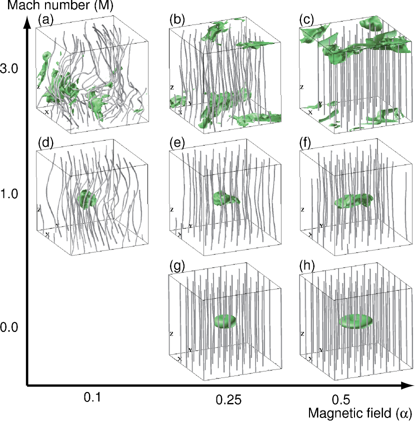
Figure 2.— Three-dimensional structures of density and magnetic fields for models with $f=1.68$. The stage $\rho_{\mathrm{max}}=10^{-8}\,\mathrm{g}\,\mathrm{cm}^{-3}$ ($n_{\mathrm{max}}=2.62\times 10^{15}\,\mathrm{cm}^{-3}$) is shown for the collapse models, while the final stage of $t=15.5t_{\mathrm{ff}}$ is shown for the non-collapse model of $(\alpha,{\cal M},f)=(0.5,3.0,1.68)$. Isosurfaces denote the iso-density surfaces of $\rho=3.16\times 10^{-20}\,\mathrm{g}\,\mathrm{cm}^{-3}$ ($n=8.28\times 10^{3}\,\mathrm{cm}^{-3}$). Tubes denote magnetic field lines. The boxes enclose the entire computational domain $(0.712~{}\mathrm{pc})^{3}$.

Figure 2 shows the cloud structures on the scale of the whole computational domain, $(0.712\,\mathrm{pc})^{3}$, at the stage with $\rho_{\mathrm{max}}=10^{-8}\,\mathrm{g}\,\mathrm{cm}^{-3}$ for the collapse models, and at $t=15.5t_{\mathrm{ff}}$ for the non-collapse model with $(\alpha,{\cal M},f)=(0.5,3.0,1.68)$. 　 The iso-density surfaces indicate the structures of the cloud cores at the low density of $\rho=3.16\times 10^{-20}\,\mathrm{g}\,\mathrm{cm}^{-3}$ ($n=8.28\times 10^{3}\,\mathrm{cm}^{-3}$), corresponding to the boundary between the cloud core and the parent cloud. The models with a high Mach number exhibit a density structure highly disturbed by the turbulence (Fig. 2a–2c), where the initial configuration of the cloud core disappears. In models with a moderate Mach number, the cloud core is strongly disturbed (Fig. 2d–2f). The models shown in Figure 2e and 2f produce cores that are flattened in the plane perpendicular to the magnetic field. The models without turbulence produce axisymmetric oblate cores flattened in the plane perpendicular to the magnetic field (Fig. 2g–2h). The magnetic field lines are highly disturbed by the turbulence in the weak-field models (Fig. 2a and 2d). In contrast, the strong-field models exhibit almost straight field lines (Fig. 2c, 2f, and 2h).

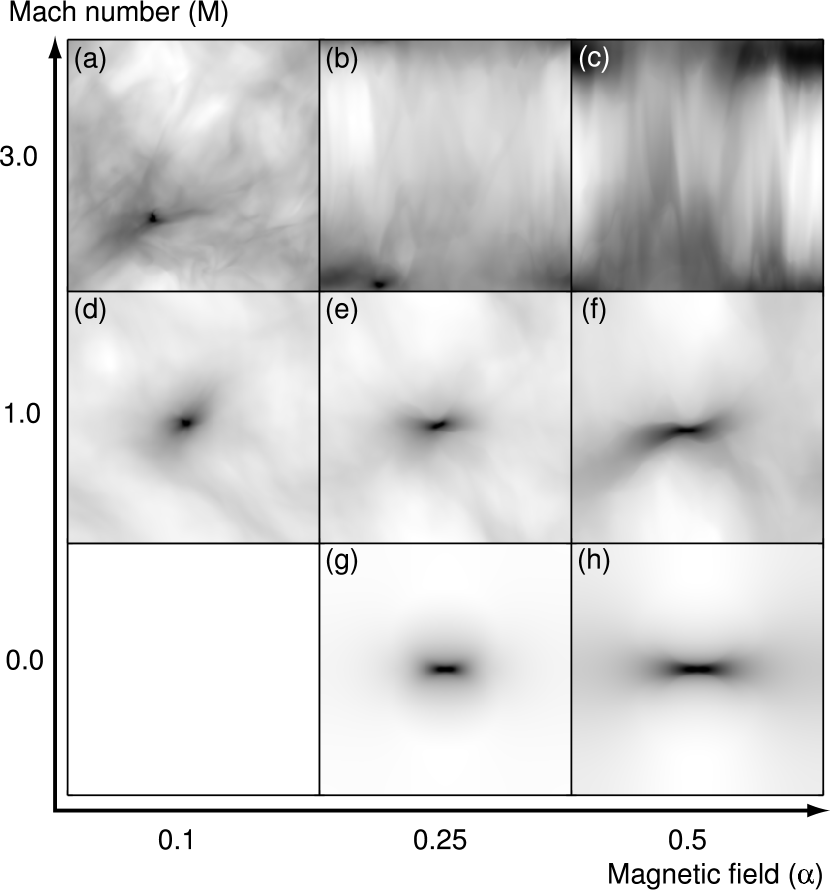
Figure 3.— Column density distributions of the entire computational domain $(0.712~{}\mathrm{pc})^{3}$ at $\rho_{\mathrm{max}}=10^{-8}\,\mathrm{g}\,\mathrm{cm}^{-3}$ ($n_{\mathrm{max}}=2.62\times 10^{15}\,\mathrm{cm}^{-3}$) for the collapse models with $f=1.68$. For the non-collapse model of $(\alpha,{\cal M},f)=(0.5,3.0,1.68)$, the final stage of $t=3.28\times 10^{6}$ yr is shown. The column densities are shown on a logarithmic scale in the $x-z$ planes.

Figure 3 shows the column density distributions of the whole computational domain for the models shown in Figure 2, clarifying the fine density distribution. The cloud cores are shown on a density scale of $n\simeq 10^{4}\,\mathrm{cm}^{-3}$, corresponding to the C¹⁸O cores. In the model with a high Mach number and weak field (Fig. 3a), the low density region is highly disturbed by the turbulence, and exhibits a complex structure. The model with a high Mach number and strong magnetic field (Fig. 3c) forms a molecular gas sheet, which lies at the top boundary of the computational domain. The location of the sheet depends on the seed of the random initial velocity field. This model shows a filamentary structure aligned parallel to the magnetic field. A similar structure was reported by Price & Bate (2008), who performed an SPH simulation taking account of the magnetic field. Nakamura & Li (2008) also reported such a filamentary structure by performing grid based MHD simulations including ambipolar diffusion. Oblate cloud cores form in Figures 3e, 3f, 3g, and 3h. The cloud cores are more flattened when the magnetic field is strong. In the turbulent models, the edges of the oblate cloud cores are warped.

At the stage shown in Figure 3, all the turbulent cloud cores move at subsonic speeds. When we define the cloud core as the gas denser than the initial ambient gas ($\rho>\rho_{0}/14$), the velocities of the baricenter of turbulent cloud cores range from 0.01 to $0.04\,\mathrm{km}\,\mathrm{s}^{-1}$. Among all the models, the model of $(\alpha,{\cal M},f)=(0.25,3.0,1.68)$ produces the first core at the most distant point (0.39 pc) from the initial peak of the cloud core.

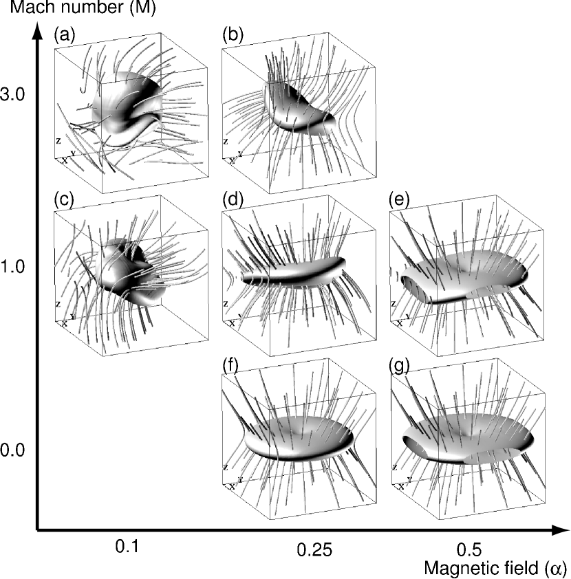
Figure 4.— Same as Figure 2 but for a $(4000~{}\mathrm{AU})^{3}$ region. Isosurfaces denote the iso-density surfaces of $\rho=10^{-17}\,\mathrm{g}\,\mathrm{cm}^{-3}$ ($n=2.62\times 10^{6}\,\mathrm{cm}^{-3}$). The model with $(\alpha,{\cal M},f)=(0.5,3.0,1.68)$ is not shown because it does not undergo collapse and the maximum density is lower than the level of the iso-surface.

Figure 4 shows the density and magnetic field in the dense regions of $(4000~{}\mathrm{AU})^{3}$ for the collapse models, showing iso-density surfaces of $\rho=10^{-17}\,\mathrm{g}\,\mathrm{cm}^{-3}$ ($n=2.62\times 10^{6}\,\mathrm{cm}^{-3}$). The cloud cores shown in this figure correspond to the dense cores observed by dust continuum emissions. Even on this scale, the weak-field models (Figs. 4a and 4c) exhibit a disturbed density structure, and the magnetic field lines are not aligned. The remaining models exhibit oblate shapes with a minor axis parallel to the local mean magnetic field. The magnetic field lines are in the configuration of an hourglass. The direction of the mean magnetic field depends on the Mach number and the magnetic field strength. The direction of the local magnetic field in models with a higher Mach number and weaker magnetic field is inclined more from that of the initial (global) magnetic field. The models of Figures 4e, 4f, and 4g exhibit mean magnetic fields parallel to the $z$-direction, while the models of Figures 4b, 4c, and 4d exhibit mean magnetic fields oriented in other directions.

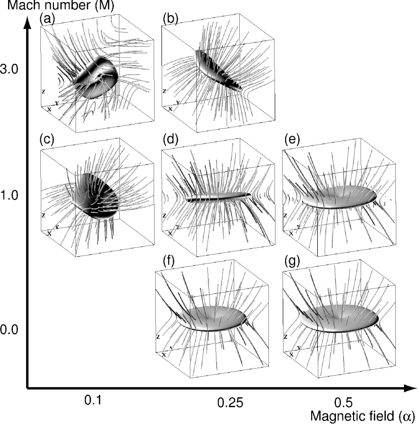
Figure 5.— Same as Figure 2 but for a $(400~{}\mathrm{AU})^{3}$ region. Isosurfaces denote the iso-density surfaces of $\rho=3.16\times 10^{-15}\,\mathrm{g}\,\mathrm{cm}^{-3}$ ($n=8.28\times 10^{8}\,\mathrm{cm}^{-3}$).

Figure 5 shows the density and the magnetic field on a 400 AU scale, showing iso-density surfaces of $\rho=3.16\times 10^{-15}\,\mathrm{g}\,\mathrm{cm}^{-3}$ ($n=8.28\times 10^{8}\,\mathrm{cm}^{-3}$). On this scale, all the models except for $(\alpha,{\cal M},f)=(0.1,3.0,1.68)$ exhibit flat disks in the plane perpendicular to the hourglass-shaped magnetic fields. The model with $(\alpha,{\cal M},f)=(0.1,3.0,1.68)$ produces a highly warped disk, and the magnetic field lines are not aligned even on this scale.

Figure 6.— Densities, magnetic fields, and outflows at the outflow formation stages for the model with $f=1.68$ in the dense region with $(40~{}\mathrm{AU})^{3}$. The stages are $\rho_{\mathrm{max}}=$ (a) $1.08\times 10^{-8}\,\mathrm{g}\,\mathrm{cm}^{-3}$, (b) $1.01\times 10^{-8}\,\mathrm{g}\,\mathrm{cm}^{-3}$, (c) $7.55\times 10^{-8}\,\mathrm{g}\,\mathrm{cm}^{-3}$, (d) $1.27\times 10^{-8}\,\mathrm{g}\,\mathrm{cm}^{-3}$, (e) $2.16\times 10^{-8}\,\mathrm{g}\,\mathrm{cm}^{-3}$, (f) $1.43\times 10^{-8}\,\mathrm{g}\,\mathrm{cm}^{-3}$, (g) $1.04\times 10^{-8}\,\mathrm{g}\,\mathrm{cm}^{-3}$. The green isosurface represents a density of $\rho=1.00\times 10^{-12}\,\mathrm{g}\,\mathrm{cm}^{-3}$ ($n=2.62\times 10^{11}\,\mathrm{cm}^{-3}$). The blue isosurface is for the radial velocity of $v_{r}=0.57\,\mathrm{km}\,\mathrm{s}^{-1}$ ($v_{r}=3c_{s}$). The tubes indicate the magnetic field lines.

Figure 6 shows the dense region on a 40 AU scale for the outflow formation stage. Four of the five turbulent collapse models produce outflows indicated by the blue isosurface of the radial velocity of $v_{r}=0.57\,\mathrm{km}\,\mathrm{s}^{-1}$ ($v_{r}=3c_{s}$). The radial velocity is measured from the location of maximum density. The outflow appears $\sim 200$ yr after the maximum density exceeds the critical density of the EOS for all the outflow models. This epoch corresponds to the stages with $\rho_{\mathrm{max}}\sim 10^{-9}\,\mathrm{g}\,\mathrm{cm}^{-3}$ for the model of Figure 6a, and $\rho_{\mathrm{max}}\sim 10^{-8}\,\mathrm{g}\,\mathrm{cm}^{-3}$ for the remaining outflow models. All the outflows are ejected in the direction parallel to the local magnetic field. The weak-field models (Figs. 6a and 6c) result in outflow directions completely different from the initial direction of the magnetic field. This is consistent with Matsumoto & Tomisaka (2004), who examined outflow formation in collapsing clouds, in which the initial magnetic field and rotation axis were not aligned. The outflows reproduced here are classified into two types: bipolar and spiral flows. The outflow shown in Figure 6a is a bipolar flow driven by tightly twisted magnetic fields. The bipolar flows in Figure 6b and 6d are accelerated by magnetic fields that are less twisted because of their higher strength. In these bipolar flows, the rotation axis of the central first core is parallel to the mean direction of the local magnetic field. The other weak-field model of Figure 6c shows a spiral flow, which is qualitatively different from the previous three outflows, showing magnetic field lines wound in a spiral shape, along which the gas is accelerated. The rotation axis of the central first core is inclined at a large angle of 35 ^∘ to the direction of the local mean magnetic field. The model shown in Figure 6e does not produce an outflow even at the final stage with $\rho=2.16\times 10^{-8}\,\mathrm{g}\,\mathrm{cm}^{-3}$. Because of the high magnetic field strength in this model, angular momentum is transferred mainly by magnetic braking instead of by outflow. The relationship between the outflow, rotation, and magnetic field are described in detail in §4.3.

Note that we reproduce the very early phase of outflow formation. At the stages shown in Figure 6, the highest outflow velocity is found for Figure 6a, exhibiting a maximum value of $v_{r}=20.7c_{s}$ ($=3.9\,\mathrm{km}\,\mathrm{s}^{-1}$). The remaining models produce maximum outflow velocities of $\sim 10c_{s}$ ($=2\,\mathrm{km}\,\mathrm{s}^{-1}$). For all models, the outflow velocity continues to increase until the end of the calculations.

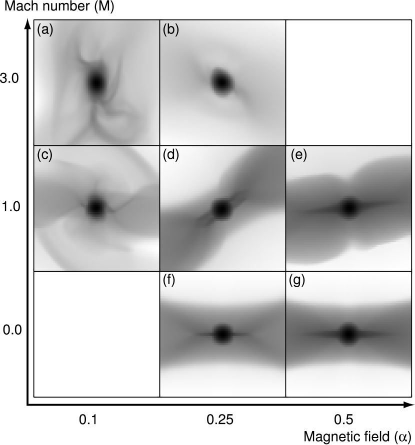
Figure 7.— Column density distributions of central $(10~{}\mathrm{AU})^{2}$ region for $\rho_{\mathrm{max}}=10^{-8}\,\mathrm{g}\,\mathrm{cm}^{-3}$. for the models with $f=1.68$. The column densities are shown on a logarithmic scale in the $x-z$ planes.

Figure 7 shows close-up views of the first cores in the column density distributions on a 10 AU scale. All the collapse models produce spherical first cores with a radius of approximately $1$ AU. The masses of the first cores are $\sim 6\times 10^{-3}\,M_{\odot}$ at the stage shown in Figure 7. All the first cores are surrounded by disk-shaped envelopes. The disk shape can be clearly seen in Figures 7d, 7e, 7f, and 7g because these disks are being viewed edge-on. The outflows disturb the disk-shaped envelope near the first cores (Fig. 7a and 7c). Note that both the first cores and the disk-shaped envelopes rotate slowly. The first cores are supported against gravity by their thermal pressure. The disk-shaped envelopes, on the other hand, are only partially supported by the centrifugal force; consequently, the infall velocity dominates over the rotation velocity. The disk-shaped envelope resembles the magnetized pseudo disk reported by Shu & Li (1997). Recently, Mellon & Li (2008, 2009) also reported that a centrifugally supported disk cannot be formed in the presence of a magnetic field due to magnetic braking.

4.1.2 Change in shape during collapse

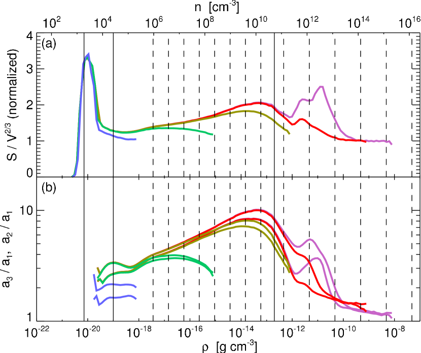
Figure 8.— (a) Normalized surface-to-volume ratios and (b) axis ratios as functions of density thresholds for the model with $(\alpha,{\cal M},f)=(0.25,1.0,1.68)$. The different colored lines correspond to the stages of $\rho_{\mathrm{max}}/\rho_{0}=10,10^{4},10^{7},10^{10}$, and $10^{11}$ ($\rho_{\mathrm{max}}=10^{-18},10^{-15},10^{-12},10^{-9},10^{-8}\,\mathrm{g}\,\mathrm{cm}^{-3}$). From left to right, the solid vertical lines represent the initial density of the ambient gas ($\rho_{0}/14.0$), the initial central density, and the critical density of the EOS ($\rho_{\mathrm{cr}}$). The dashed vertical lines represent the densities at which grid refinement was carried out according to the Jeans condition.

In order to measure the complexity of the density distribution during the collapse, we evaluate the surface-to-volume ratio and axis ratios for a given iso-density surface according to Appendix B. The surface-to-volume ratio is normalized so that it has a value of unity for a sphere. Figure 8 shows surface-to-volume ratios for the model with $(\alpha,{\cal M},f)=(0.25,1.0,1.68)$ as a fiducial model. In the early stage with $\rho_{\mathrm{max}}=10^{-18}\,\mathrm{g}\,\mathrm{cm}^{-3}$ (blue curves), the iso-surfaces of $\rho\simeq 10^{-20}\,\mathrm{g}\,\mathrm{cm}^{-3}$ have high surface-to-volume ratios, indicating that the cloud core has a complex density distribution in the low density region. The surface-to-volume ratio vanishes below the minimum density. This is because the isosurface vanishes there while the volume coincide with that of the whole computation box because of the periodic boundary condition. In contrast, the iso-surface of $\rho\sim 10^{-18}\,\mathrm{g}\,\mathrm{cm}^{-3}$ exhibits a low surface-to-volume ratio, and $a_{3}$ is considerably longer than $a_{2}$. This indicates that the collapsing region has a smooth triaxial shape at this stage. Note that the vertical dashed lines denote the densities at which the grid refinements are performed. At low densities, the surface-to-volume ratio is seen to make a transition from a high to a low value. Since this occurs at a density less than that of the first refinement, it cannot be attributed to the grid refinement process. At the stage with $\rho_{\mathrm{max}}=10^{-15}\,\mathrm{g}\,\mathrm{cm}^{-3}$ (green curves), the two axis ratios have an identical value of $3-4$, indicating that the collapsing region of the cloud core is an almost axisymmetric disk. Owing to its flat shape, the surface-to-volume ratio is slightly higher than unity for $\rho\sim 10^{-17}\,\mathrm{g}\,\mathrm{cm}^{-3}$. At the stage with $\rho_{\mathrm{max}}=10^{-12}\,\mathrm{g}\,\mathrm{cm}^{-3}$ (yellow curves), the surface-to-volume ratio reaches 1.8 at $\rho\simeq 10^{-14}\,\mathrm{g}\,\mathrm{cm}^{-3}$, and the axis ratios reach $7-8$, indicating that the flatness of the disk increases during the collapse. At the stage with $\rho_{\mathrm{max}}=10^{-9}\,\mathrm{g}\,\mathrm{cm}^{-3}$ (red curves), a spherical first core forms, and the surface-to-volume ratio and axis ratios become unity at the high density of $\rho\gtrsim 10^{-10}\,\mathrm{g}\,\mathrm{cm}^{-3}$. The surface-to-volume ratio and the axis ratios of the disk-shaped envelope reach 2 and 10, respectively, at $\rho\simeq 10^{-13}\,\mathrm{g}\,\mathrm{cm}^{-3}$ owing to an increase in the flatness. At the outflow formation stages (purple curves), the surface-to-volume ratio takes a high value of 2.5 at $\rho\simeq 10^{-11}\,\mathrm{g}\,\mathrm{cm}^{-3}$, reflecting the fact that the outflow disturbs the disk-shaped envelope around the first core. The surface-to-volume ratio and the axis ratios remain unity in the dense region with $\rho\gtrsim 10^{-10}\,\mathrm{g}\,\mathrm{cm}^{-3}$, indicating that the first core is spherical even at the outflow formation stage. Moreover, at the low density region with $\rho\simeq 10^{-20}\,\mathrm{g}\,\mathrm{cm}^{-3}$, the surface-to-volume ratio remains high even after first core formation, indicating that the periphery of the cloud core remains turbulent.

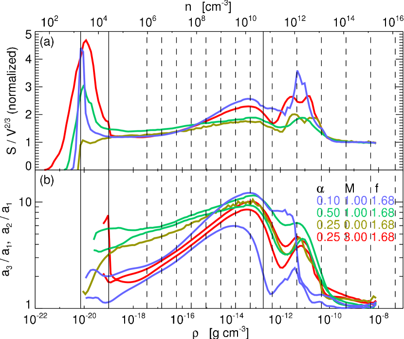
Figure 9.— (a) Normalized surface-to-volume ratios and (b) axis ratios as functions of density thresholds for the models with $f=1.68$ at the stage with $\rho_{\mathrm{max}}=10^{-8}\,\mathrm{g}\,\mathrm{cm}^{-3}$. The different colored lines correspond to the different models. From left to right, the solid vertical lines represent the initial density of the ambient gas ($\rho_{0}/14.0$), the initial central density, and the critical density of the EOS ($\rho_{\mathrm{cr}}$). The dashed vertical lines represent the densities at which grid refinement was carried out according to the Jeans condition.

Figure 9 compares the surface-to-volume ratio and the axis ratios for the four models with $f=1.68$. For a low density of $\rho\lesssim 10^{-19}\,\mathrm{g}\,\mathrm{cm}^{-3}$, the turbulent models exhibit high surface-to-volume ratios. The model with a high Mach number (${\cal M}=3$) exhibits the highest value (red curve), while the model without turbulence exhibits a low ratio (yellow curve). Comparing the models with ${\cal M}=1$, the weak-field model (blue curve) has a higher surface-to-volume ratio than the strong-field model (green curve), implying that disturbance by turbulent flow is considerably suppressed by the magnetic field.

In all the models, the axis ratios increase with density in the range of $10^{-18}\,\mathrm{g}\,\mathrm{cm}^{-3}\lesssim\rho\lesssim 10^{-13}\,\mathrm{g}\,\mathrm{cm}^{-3}$. In this range, the mean axis ratios $(a_{2}+a_{3})/(2a_{1})$ tend to increase with the initial magnetic filed strength $\alpha$, and decrease with the initial Mach number ${\cal M}$. This implies that the magnetic field increases the degree of anisotropy and the turbulence increases the effective sound speed. This tendency is apparent at a relatively low density of $10^{-18}\,\mathrm{g}\,\mathrm{cm}^{-3}\lesssim\rho\lesssim 10^{-15}\,\mathrm{g}\,\mathrm{cm}^{-3}$.

At $\rho\sim 10^{-13}\,\mathrm{g}\,\mathrm{cm}^{-3}$, the model with $(\alpha,{\cal M},f)=(0.1,1.0,1.68)$ exhibits a prolate shape (blue curves), with the major axis being considerably longer than the other axes; the axis ratio $a_{3}/a_{2}$ has a maximum of 6.2 at $\rho=3.8\times 10^{-13}\,\mathrm{g}\,\mathrm{cm}^{-3}$. For all the other models, the axes $a_{3}$ and $a_{2}$ are comparable ($a_{3}/a_{2}<2$) for $\rho\geq 10^{-17}\,\mathrm{g}\,\mathrm{cm}^{-3}$, indicating an oblate shape. For a higher density of $\rho\gtrsim 10^{-11}\,\mathrm{g}\,\mathrm{cm}^{-3}$, all the models exhibit spherical shapes because of the presence of the first cores.

4.2. Dependence on mass

We examined two additional models with $f=3.0$ and 6.0 in order to investigate the dependence on cloud mass. We refer to these models as massive cloud cores. The parameters of the initial magnetic field and the initial Mach number of turbulence are $\alpha=0.1$ and ${\cal M}=3.0$, respectively. It takes shorter time to form first core for the more massive core; the first core forms at $t=5.24t_{\mathrm{ff}}$ for a model with $(\alpha,{\cal M},f)=(0.1,3.0,1.68)$, and at $t=1.29t_{\mathrm{ff}}$ for a model with $(\alpha,{\cal M},f)=(0.1,3.0,6.0)$.

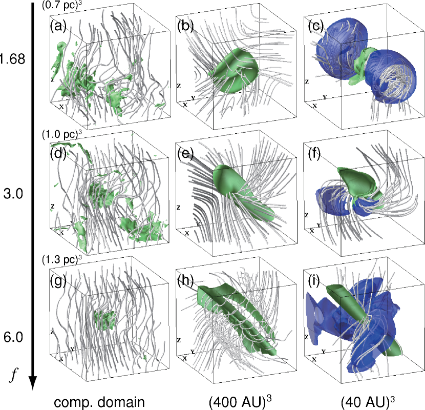
Figure 10.— Three-dimensional structures of density, magnetic fields, and outflows for the models with $(\alpha,{\cal M},f)=(0.1,3.0,1.68)$, $(0.1,3.0,3.0)$, and $(0.1,3.0,6.0)$ from top to bottom. From left to right, the plotted areas are the entire computation box, $(400~{}\mathrm{AU})^{3}$, and $(40~{}\mathrm{AU})^{3}$. From left to right, the isosurfaces denote the iso-density surfaces of $\rho=3.16\times 10^{-20}\,\mathrm{g}\,\mathrm{cm}^{-3}$, $3.16\times 10^{-15}\,\mathrm{g}\,\mathrm{cm}^{-3}$, and $1.00\times 10^{-12}\,\mathrm{g}\,\mathrm{cm}^{-3}$. Tubes denote magnetic field lines. The blue isosurface is for a radial velocity of $v_{r}=0.57\,\mathrm{km}\,\mathrm{s}^{-1}$ ($v_{r}=3c_{s}$). The stages are $\rho_{\mathrm{max}}=4.53\times 10^{-8}\,\mathrm{g}\,\mathrm{cm}^{-3}$ for panel f, and $\rho_{\mathrm{max}}=10^{-8}\,\mathrm{g}\,\mathrm{cm}^{-3}$ for the rest of the panels.

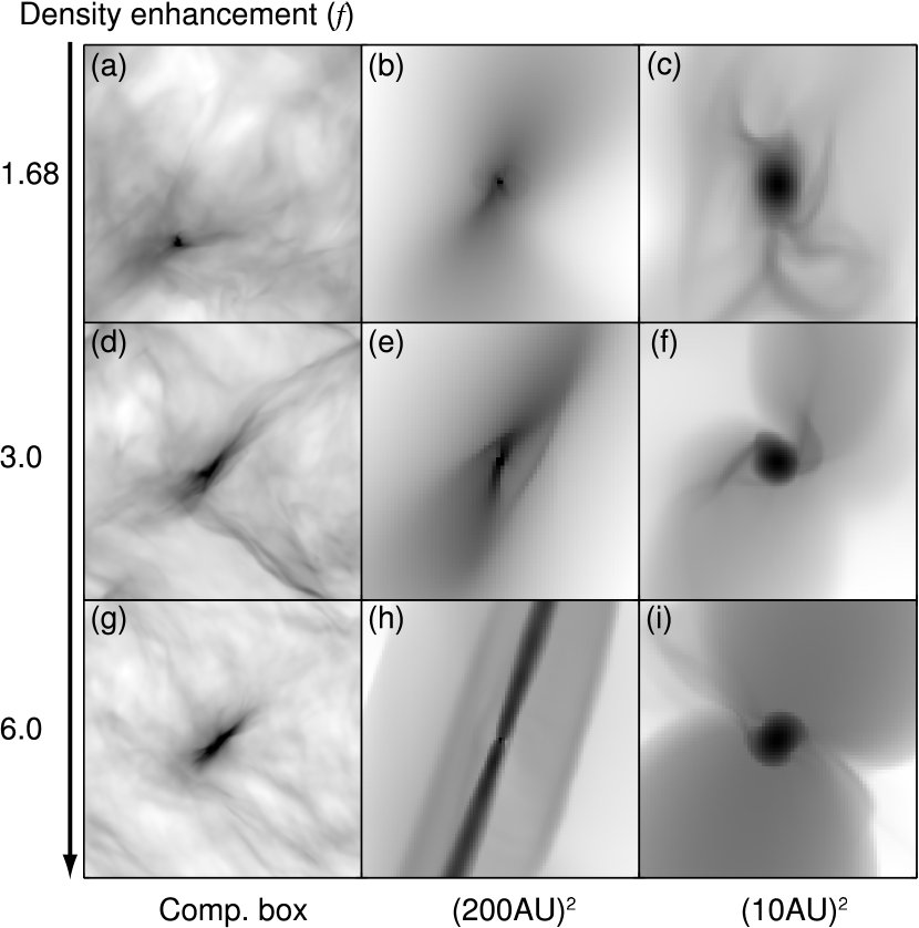
Figure 11.— Column density distributions at the stage with $\rho_{\mathrm{max}}=10^{-8}\,\mathrm{g}\,\mathrm{cm}^{-3}$ for the models with $(\alpha,{\cal M},f)=(0.1,3.0,1.68)$, $(0.1,3.0,3.0)$, and $(0.1,3.0,6.0)$ from top to bottom. The column densities are shown on a logarithmic scale in the $x-z$ planes. From left to right, the plotted regions are the whole computational domains, $(200~{}\mathrm{AU})^{2}$, $(10~{}\mathrm{AU})^{2}$.

Figures 10 and 11 compare the three models on three spatial scales. The low density regions are highly disturbed by the turbulence in all the models (left column in Figs. 10 and 11). On the intermediate scale (the middle column), the clouds take the shape of filaments for the massive models. The most massive model produces a long thin filament as shown in Figures 10h and 11h. On the small scale, all the models produce spherical first cores (right column in Fig. 11). The first cores of the massive clouds are embedded in the filament, while that of the less massive cloud is surrounded by the disk (right column in Figs. 10).

All the models exhibit outflows as shown by the blue iso-velocity surfaces in Figure 10, but their shapes are different. The outflow shown in Figure 10c is classified as bipolar flow, and it is ejected in the direction perpendicular to the plane of the disk. The disk-outflow system is roughly axisymmetric although its axis is inclined considerably with respect to the initial direction of the magnetic field (the vertical direction). In the massive models with $f=3.0$ and 6.0 (Figs. 10f and 10i), the outflow is classified as spiral flow, and it is ejected in the plane perpendicular to the filament, and is not collimated. Similar outflow appears for the model with $(\alpha,{\cal M},f)=(0.1,1.0,1.68)$ as shown in Figure 6c. The configuration of the magnetic field depends on the type of outflow present. In the less massive model with $f=1.68$, the magnetic field lines are twisted and highly wound along the bipolar directions, implying that the outflow is accelerated by the magnetic pressure. In the massive models, the magnetic field lines exhibit a spiral configuration, which is attributed to misalignment between the rotation axis and the local mean magnetic field. This morphology implies that the outflow is accelerated by magnetic tension.

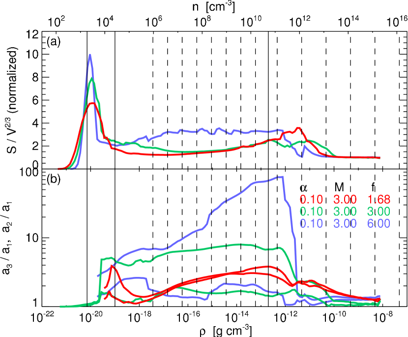
Figure 12.— (a) Normalized surface-to-volume ratios and (b) axis ratios as functions of density thresholds for the models with ${\cal M}=3$ and $\alpha=0.1$. From left to right, the solid vertical lines represent the initial density of the ambient gas ($\rho_{0}/14.0$), the initial central density, and the critical density of the EOS ($\rho_{\mathrm{cr}}$). The dashed vertical lines represent the densities at which grid refinement was carried out according to the Jeans condition.

Figure 12 compares the surface-to-volume ratio and axis ratios for the three models. Even for the same initial Mach number, low-density regions with $\rho\simeq 10^{-20}\,\mathrm{g}\,\mathrm{cm}^{-3}$ are more disturbed in the more massive model, showing a higher surface-to-volume ratio (Fig. 12a). The less massive model produces a disk-shaped envelope in the range $10^{-17}\,\mathrm{g}\,\mathrm{cm}^{-3}\lesssim\rho\lesssim 10^{-12}\,\mathrm{g}\,\mathrm{cm}^{-3}$, indicated by the identical values of the two axis ratios (red curves in Fig. 12b). In contrast, the massive clouds produce a filamentary envelope. The axis ratio $a_{3}/a_{1}$ reaches a maximum value of $\simeq 80$ for the most massive model (blue curves in Fig. 12b). For $\rho\gtrsim 10^{-10}\,\mathrm{g}\,\mathrm{cm}^{-3}$, the surface-to-volume ratio and the axis ratios are almost unity, irrespective of the cloud masses because of the spherical first cores.

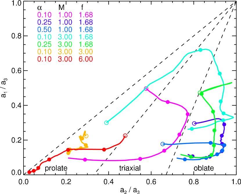
Figure 13.— Distribution of axis ratio for the isothermal range ($\rho_{0}\leq\rho\leq\rho_{\mathrm{cr}}$) at the stage with $\rho_{\mathrm{max}}=10^{-8}\,\mathrm{g}\,\mathrm{cm}^{-3}$ for all the collapse models with turbulence (${\cal M}\neq 0$). The open circles denote the axis ratios at $\rho=\rho_{0}$. The filled circles denote the axis ratios at $\rho=10^{n}\rho_{0}$ ($n=1,2,\cdots,6$). The dashed lines indicate the boundary between prolate, triaxial, and oblate shapes.

Figure 13 shows the distribution of the axis ratios of the isothermal envelopes ($\rho_{0}\leq\rho\leq\rho_{\mathrm{cr}}$). Based on the axis ratios, the shapes of the envelopes are divided into three categories: prolate, triaxial, and oblate (Gammie et al., 2003). In all the collapse models, the shape anisotropy increases ($a_{1}/a_{3}$ decreases) with the density threshold for $\rho\gtrsim 10\rho_{0}$ ($=10^{-18}\,\mathrm{g}\,\mathrm{cm}^{-3}$). All the massive cloud cores with $f=3.0$ and 6.0 have prolate shapes, with $a_{2}/a_{3}$ and $a_{1}/a_{3}$ decreasing with increasing density threshold. Four of the five less massive cloud cores with $f=1.68$ produce oblate cores for $\rho>100\rho_{0}$. In addition, the evolutionary tracks of the axis ratios for the dense regions ($\rho\geq\rho_{\mathrm{max}}/10$) exhibit loci similar to those shown in Figure 13, indicating that the shapes of the envelopes reflect the history of the collapse. In summary, massive cloud cores tend to have a prolate shape, and less massive cores an oblate shape.

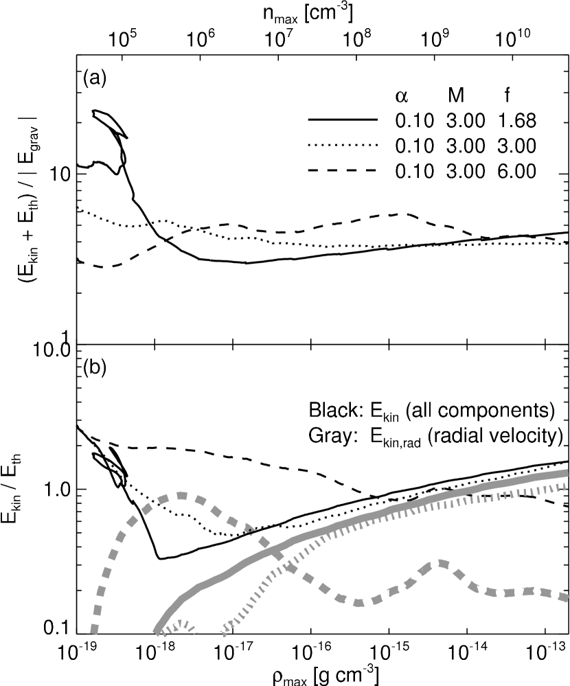
Figure 14.— Energy ratios (a) $(E_{\mathrm{kin}}+E_{\mathrm{th}})/|E_{\mathrm{grav}}|$ and (b) $E_{\mathrm{kin}}/E_{\mathrm{th}}$ as functions of the maximum density $\rho_{\mathrm{max}}$ in the isothermal collapse phase for the models with ${\cal M}=3$ and $\alpha=0.1$. Solid, dotted, and dashed lines correspond to models with $f=1.68$, 3.0, and 6.0, respectively. Gray lines in the panel (b) denote the ratios of the kinetic energy of the radial velocity to the thermal energy $E_{\mathrm{kin,rad}}/E_{\mathrm{th}}$.

In order to investigate the deformation of the cloud cores, we consider the kinetic, thermal, and gravitational energy of the dense regions during the collapse. Figure 14a shows $(E_{\mathrm{kin}}+E_{\mathrm{th}})/|E_{\mathrm{grav}}|$ in the dense region with $\rho\geq 0.1\rho_{\mathrm{max}}$ during the isothermal collapse phase ($\rho_{0}\leq\rho_{\mathrm{max}}\leq\rho_{\mathrm{cr}}$). These energies are estimated as $E_{\mathrm{kin}}=(1/2)\int_{\rho\geq 0.1\rho_{\mathrm{max}}}\rho|\mbox{\boldmath$v$}|^{2}dV$, $E_{\mathrm{th}}=(3/2)\int_{\rho\geq 0.1\rho_{\mathrm{max}}}PdV$, and $|E_{\mathrm{grav}}|=(1/8\pi G)\int_{\rho\geq 0.1\rho_{\mathrm{max}}}|\mbox{\boldmath$g$}|^{2}dV$. As shown in Figure 14a, the values of the energy ratio $(E_{\mathrm{kin}}+E_{\mathrm{th}})/|E_{\mathrm{grav}}|$ converge to $\sim 4$ by the early stage with $\rho_{\mathrm{max}}\simeq 10^{-18}\,\mathrm{g}\,\mathrm{cm}^{-3}$, and remain roughly constant during the isothermal collapse. This convergence is explained by the virial theorem, which predicts that $(E_{\mathrm{kin}}+E_{\mathrm{th}}+E_{\mathrm{mag}}/2)/|E_{\mathrm{grav}}|\simeq 1/2$. The overestimation in Figure 14a is attributed to the underestimation of the gravitational energy, since we ignored the contribution of the low density regions.

Figure 14b shows the energy ratio, $E_{\mathrm{kin}}/E_{\mathrm{th}}$, during the isothermal collapse. For $\rho_{\mathrm{max}}\lesssim 10^{-15}\,\mathrm{g}\,\mathrm{cm}^{-3}$, the kinetic energy exceeds the thermal energy for the most massive model with $f=6$ (thin dashed curve), and vice verse for the less massive model with $f=1.68$ (thin solid curve). The massive cloud core is supported mainly by the turbulence, and it collapses to form a filament. In contrast, the oblate shape in the less massive model is attributed to thermal pressure support.

In the early phase, the energy ratio $E_{\mathrm{kin}}/E_{\mathrm{th}}$ decreases for all the models. However, they begin to increase at $\rho_{\mathrm{max}}=10^{-18}\,\mathrm{g}\,\mathrm{cm}^{-3}$ for the model with $f=1.68$ and at $10^{-17}\,\mathrm{g}\,\mathrm{cm}^{-3}$ for the model with $f=3$. This increase is attributed to an increase in the infall energy, as indicated by the gray curves, which denote the energy ratio $E_{\mathrm{kin,rad}}/E_{\mathrm{th}}$, where $E_{\mathrm{kin,rad}}$ is the kinetic energy associated only with the radial velocity, and is defined by $E_{\mathrm{kin,rad}}=(1/2)\int_{\rho\geq 0.1\rho_{\mathrm{max}}}\rho v_{r}^{2}dV$. For $\rho_{\mathrm{max}}\gtrsim 10^{-16}\,\mathrm{g}\,\mathrm{cm}^{-3}$, the energy of infall motion dominates over the turbulent energy for the models with $f=1.68$ and 3.0.

4.3. Outflow, rotation, and magnetic field

As shown in §4.1 and §4.2, the models examined here exhibit either bipolar or spiral outflow. Examples of bipolar flows are shown in Figures 6a, 6b, and 6d, and spiral flows in Figures 6c, 10f and 10i. The bipolar outflows tend to be associated with disk-shaped envelopes, while the spiral flows tend to have filamentary envelopes.

In order to investigate the relationship between the rotation and magnetic field, we calculate the angular momentum ($J$) and the mean magnetic field ($\bar{\mbox{\boldmath$B$}}$) for $\rho\geq 0.1\rho_{\mathrm{max}}$ during the collapse (see Appendix C). The angular momentum can be decomposed into two components parallel and perpendicular to the mean magnetic field, defined by

$$J_{\parallel}=|\mbox{\boldmath$J$}\cdot\bar{\mbox{\boldmath$B$}}|/|\bar{\mbox{\boldmath$B$}}|,$$ (3)

and

$$J_{\perp}=|\mbox{\boldmath$J$}\times\bar{\mbox{\boldmath$B$}}|/|\bar{\mbox{\boldmath$B$}}|.$$ (4)

It should be pointed out that the region of interest $\rho\geq 0.1\rho_{\mathrm{max}}$ changes temporally. Therefore, changes in $J$ and $\bar{\mbox{\boldmath$B$}}$ do not indicate temporal changes in the angular momentum and magnetic field of the fixed regions, but rather they trace the angular momentum and magnetic field in the collapsing region.

Figure 15.— Normalized angular momentum ($J/M^{2}[c_{s}/4\pi G]$) within the dense region with $\rho\geq 0.1\rho_{\mathrm{max}}$ as a function of the maximum density $(\rho_{\mathrm{max}})$ for the model with $(\alpha,{\cal M},f)=(0.25,1.0,1.68)$. The angular momentum $J/M^{2}$ is plotted as a thin solid curve, while the parallel and perpendicular components of angular momentum with respective to the local magnetic field, $J_{\parallel}/M^{2}$ and $J_{\perp}/M^{2}$, are plotted as thin dashed and thin dotted curves, respectively. The thick solid curve denotes the angle $\theta_{\mathrm{01}}$ between the vectors of the angular momentum $J$ and the mean local magnetic field $\bar{\mbox{\boldmath$B$}}$ for the region with $\rho\geq 0.1\rho_{\mathrm{max}}$, while the thick dashed curve denotes the angle $\theta_{\mathrm{cr}}$, which is same as $\theta_{\mathrm{01}}$ but for the region of $\rho\geq\rho_{\mathrm{cr}}$. Both angles are restricted to within $[0,90]$ degrees. The vertical line denotes the critical density of the EOS, $\rho_{\mathrm{cr}}$.

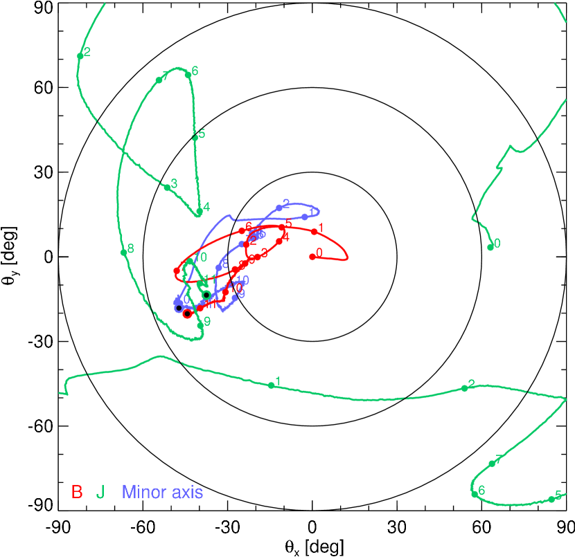
Figure 16.— Loci of the directions of the mean magnetic field $\pm\bar{\mbox{\boldmath$B$}}$ (red line), the angular momentum $\pm\mbox{\boldmath$J$}$ (green line), and the minor axis of the density structure (blue line) in the region with $\rho\geq 0.1\rho_{\mathrm{max}}$ for the model with $(\alpha,{\cal M},f)=(0.25,1.0,1.68)$. Digits $n$ with filled circles denote the stages of $\rho_{\mathrm{max}}=10^{n}\rho_{0}$. Black filled circles denote the final stage. The three large circles denote the relationships $(\theta_{x}^{2}+\theta_{y}^{2})^{1/2}=30^{\circ}$, $60^{\circ}$, and $90^{\circ}$.

Figure 15 shows $J/M^{2}$, $J_{\parallel}/M^{2}$, and $J_{\perp}/M^{2}$ as functions of $\rho_{\mathrm{max}}$ for the model with $(\alpha,{\cal M},f)=(0.25,1.0,1.68)$, the representative model of a bipolar outflow. The ordinate $J/M^{2}$ is nearly equal to the specific angular momentum per unit mass $j/M$, which remains constant as the disk-like cloud collapses in the cylindrical radial direction (see e.g., Matsumoto et al., 1997). For a slowly rotating non-magnetized cloud, $J/M^{2}$ increases slightly with density because of a slight spin-up due to spherical collapse (see Fig. 4 in Matsumoto & Tomisaka, 2004).

In isothermal collapse ($\rho_{\mathrm{max}}\leq\rho_{\mathrm{cr}}$), $J/M^{2}$ decreases slightly with a considerable amount of oscillation. The slight decrease in the $J/M^{2}$ is attributed to magnetic braking. In the early phase with $\rho_{\mathrm{max}}\lesssim 10^{-16}\,\mathrm{g}\,\mathrm{cm}^{-3}$, the perpendicular component, $J_{\perp}$, is larger than the parallel component, $J_{\parallel}$, and exhibits a large value of $\theta_{01}$, which is the angle between $J$ and $\bar{\mbox{\boldmath$B$}}$, and it is restricted to values from $0$ to $90^{\circ}$. The angle $\theta_{01}$ therefore becomes 0 when $J$ and $\bar{\mbox{\boldmath$B$}}$ are either parallel or anti-parallel. In the range of $10^{-16}\,\mathrm{g}\,\mathrm{cm}^{-3}\lesssim\rho_{\mathrm{max}}\lesssim 10^{-14}\,\mathrm{g}\,\mathrm{cm}^{-3}$, $J_{\perp}$ is smaller than $J_{\parallel}$, and $\theta_{01}$ also becomes smaller. When the EOS becomes adiabatic ($\rho_{\mathrm{max}}=\rho_{\mathrm{cr}}$), $J_{\perp}$ is larger than $J_{\parallel}$. Also plotted in Figure 15 is another angle $\theta_{\mathrm{cr}}$, which is the angle between the angular momentum and the magnetic filed for the region with $\rho\geq\rho_{\mathrm{cr}}$. After the EOS becomes adiabatic ($\rho_{\mathrm{max}}\geq\rho_{\mathrm{cr}}$), the angle $\theta_{\mathrm{cr}}$ remains constant. In contrast, $\theta_{01}$ decreases up to $\sim 5^{\circ}$ by the final stage, indicating that the rotation axis is aligned with the magnetic field in the dense region. Moreover, the angular momentum $J/^{2}M$ decreases. The perpendicular component decreases selectively by more than an order of magnitude. This indicates that the magnetic braking is more effective against the perpendicular component of angular momentum with respective to the local magnetic field than the parallel component. Such selective magnetic braking is also reported in Matsumoto & Tomisaka (2004).

Figure 16 shows the loci of the directions of the mean magnetic field $\bar{\mbox{\boldmath$B$}}$, the angular momentum $J$, and the minor axis of the density structure (the normal vector of the disk) in the region with $\rho\geq 0.1\rho_{\mathrm{max}}$ for the model with $(\alpha,{\cal M},f)=(0.25,1.0,1.68)$. Each vector is plotted in the two-dimensional plane as

$$\left(\begin{array}[]{c}\theta_{x}\\ \theta_{y}\end{array}\right)=\frac{\arctan(V_{xy}/V_{z})}{V_{xy}}\left(\begin{array}[]{c}V_{x}\\ V_{y}\end{array}\right),$$ (5)

where $\mbox{\boldmath$V$}=(V_{x},V_{y},V_{z})$ represents a given vector and $V_{xy}=(V_{x}^{2}+V_{y}^{2})^{1/2}$. The distance from the origin represents the angle between a given vector and the $z$-axis. For example, a vector parallel to the $x$-axis is plotted at $(90^{\circ},0)$. The direction of the magnetic field and the minor axis of the density structure are aligned during the collapse, suggesting that the cloud collapses along the magnetic field lines, and the disk is oriented always perpendicular to the local magnetic field. The direction of the angular momentum drifts considerably over the $\theta_{x}-\theta_{y}$ plane, while it begins to be aligned with the magnetic field and the minor axis at $\rho_{\mathrm{max}}/\rho_{0}\sim 10^{8}$ ($\rho_{\mathrm{max}}=10^{-11}\,\mathrm{g}\,\mathrm{cm}^{-3}$). Finally, for $\rho_{\mathrm{max}}/\rho_{0}\gtrsim 10^{10}$ ($\rho_{\mathrm{max}}=10^{-8}\,\mathrm{g}\,\mathrm{cm}^{-3}$), all three vectors are aligned at the point $(\theta_{x},\theta_{y})\simeq(-40^{\circ},-20^{\circ})$. This alignment produces the bipolar outflow.

Figure 17.— Same as figure 15 but for the model with $(\alpha,{\cal M},f)=(0.1,3.0,1.68)$.

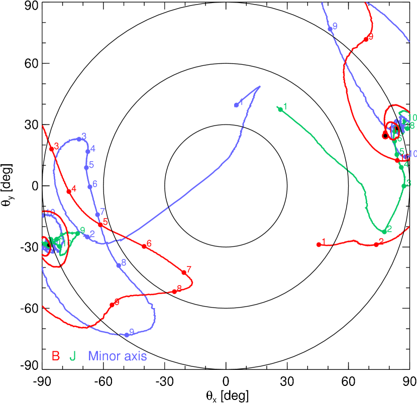
Figure 18.— Same as figure 16 but for the model with $(\alpha,{\cal M},f)=(0.1,3.0,1.68)$. The loci are shown for $\rho_{\mathrm{max}}/\rho_{0}\geq 10$, because they are noisy below that stage.

Figure 17 is same as Figure 15 but for the model with with $(\alpha,{\cal M},f)=(0.1,3.0,1.68)$, where the most prominent bipolar outflow appears. In the early stage with $\rho_{\mathrm{max}}\lesssim 10^{-18}\,\mathrm{g}\,\mathrm{cm}^{-3}$, the angular momentum strongly oscillates due to the strong turbulence and the weak magnetic field. After the collapse proceeds, $J/M^{2}$ remains roughly constant in the isothermal collapse phase ($\rho_{\mathrm{max}}\leq\rho_{\mathrm{cr}}$). In this phase, the direction of the angular momentum changes considerably as shown in Figure 18. The weak magnetic field changes its direction significantly due to precession. The disk normal follows the magnetic field, so that the plane of the disk remains perpendicular to the magnetic field. In the adiabatic phase ($\rho_{\mathrm{max}}\geq\rho_{\mathrm{cr}}$), $J/M^{2}$ deceases with increasing density as shown in Figure 17. The perpendicular component $J_{\perp}/M^{2}$ decreases drastically as in the previous model. This model therefore results in alignment of the rotation axis with the local magnetic field, with $\theta_{01}\sim 0$ in the final stage. This alignment is also shown in Figure 18, where the directions of the magnetic field, the angular momentum, and the disk normal converge at the point $(\theta_{x},\theta_{y})\simeq(80^{\circ},30^{\circ})$, that is almost perpendicular to the $z$ axis. The angular momentum $J/M^{2}$ is about five times larger than that for the previous model throughout its evolution (compare Figs.15 and 17), and this model exhibits strong outflow. The large angular momentum is attributed to both the initial strong turbulence and the weak magnetic field.

Figure 19.— Same as figure 15 but for the model with $(\alpha,{\cal M},f)=(0.1,3.0,3.0)$.

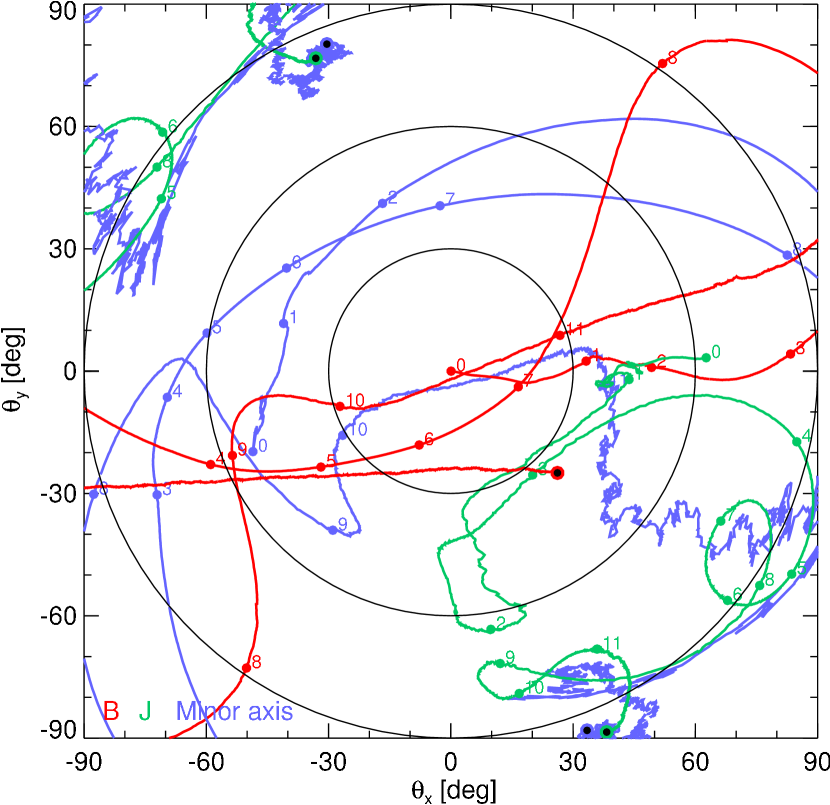
Figure 20.— Same as figure 16 but for the model with $(\alpha,{\cal M},f)=(0.1,3.0,3.0)$.

Figure 19 shows the evolution of angular momentum for the model with $(\alpha,{\cal M},f)=(0.1,3.0,3.0)$, a typical model showing a spiral flow. In this model, the angular momentum and magnetic field are not aligned throughout the evolution. The angle $\theta_{01}$ increases and exhibits large oscillations. The angular momentum $J/M^{2}$ remains roughly constant in the isothermal collapse phase ($\rho_{\mathrm{max}}\leq\rho_{\mathrm{cr}}$), while it decreases in the adiabatic phase ($\rho_{\mathrm{max}}\geq\rho_{\mathrm{cr}}$). The perpendicular component $J_{\perp}$ is considerably larger than the parallel component $J_{\parallel}$ in the adiabatic phase, producing large $\theta_{01}$ and $\theta_{\mathrm{cr}}$ values.

The magnetic field, the angular momentum, and the minor axis evolve completely differently in the spiral models as shown in Figure 20. The locus of $J$ moves in the lower right direction with a large precession. The locus of $\bar{\mbox{\boldmath$B$}}$ moves diagonally from lower left to upper right, indicating that the orientation of $\bar{\mbox{\boldmath$B$}}$ rotates around $J$. The point $\bar{\mbox{\boldmath$B$}}$ traverses the $\theta_{x}-\theta_{y}$ plane three times, indicating that it makes 1.5 revolutions. The minor axis follows the direction of the magnetic field in the stage with $\rho_{\mathrm{max}}\lesssim 10^{11}\rho_{0}$ ($\rho_{\mathrm{max}}\lesssim 10^{-8}\,\mathrm{g}\,\mathrm{cm}^{-3}$), while it follows the direction of the angular momentum in the stage with $\rho_{\mathrm{max}}\gtrsim 10^{11}\rho_{0}$ ($\rho_{\mathrm{max}}\gtrsim 10^{-8}\,\mathrm{g}\,\mathrm{cm}^{-3}$). In the final stage, the angular momentum and the minor axis are aligned at the point $(\theta_{x},\theta_{y})\simeq(-30^{\circ},80^{\circ})$. This indicates that the filaments shown in Figure 10e and Figure 11e are perpendicular to the magnetic fields, while the first core shown in Figure 11e is slightly oblate, with its minor axis oriented parallel to the rotation axis.

5. Discussion

5.1. Shape of cloud core

Cloud core shape is investigated quantitatively by means of the surface-to-volume ratio and axis ratios (Figs. 8, 9, and 12). In all the models with turbulence, a cloud core has a complex density distribution before it begins to collapse. In contrast, the density distribution is relatively smooth in a collapsing cloud core, which is partly due to decay of turbulence before collapse. Strong turbulence prohibits cores from collapsing. In other words, the decay of turbulence promotes collapse in particular in a less massive core (Fig. 1). A dense core begins to collapse when the turbulence decays to a certain level depending on the core mass. A less massive core does not collapse until the turbulence decays to a very low level. Accordingly the collapsing cores tend to have a smooth density distribution. We also note that it takes a longer time before collapse if the initial turbulence is stronger. This is one of the reasons why the density distribution is relatively smooth in the first cores formed in our simulations.

The above argument, however, does not hold for a massive cloud core, which collapses rapidly before decay of turbulence (Fig. 14). Even when a core forms before the decay of turbulence, it has a relatively smooth density distribution. We suppose that this is due to shrink of the core. The diameter of a collapsing core is about the Jeans length, which decreases in proportion to $\rho^{-1/2}$ during the runaway collapse if the gas is isothermal. Turbulence supports a core against collapse only when the typical wavelength is shorter than the diameter of the cloud. Turbulence has a smaller power at a shorter wavelength in our initial model as well as in the Kolmogorov spectrum. Accordingly the effective level of turbulence decreases along with the shrink of the core, unless the wavelength of the turbulence shortens in proportion to the Jeans length. The wavelength of turbulence may be shortened a little by compression and advection, but not much. Remember that the core mass decreases during the runaway collapse. This means that the advection is slower than the collapse. The above mentioned idea is supported by the fact that the turbulence is still strong in the low density region even after the collapse (Fig. 12).

Consequently, the turbulence introduces only smooth motion, e.g., rotation and shear, into the collapsing region. Our results are in agreement with observations of starless dense cores with molecular line emissions (e.g., Goodman et al., 1998; Tafalla et al., 2002), which suggest that turbulent motion decreases toward the center of the cloud core and coherent motion remains at the central part. For star-forming cores, the internal structure may be produced by the activation of young stars, e.g., outflows from young stars and the orbital motion of a multiple system (c.f., Wang et al., 2010).

The shape of the collapsing region depends mainly on the mass of the cloud core, and the orientation is controlled by the magnetic fields. In the less massive cloud core, the collapsing region assumes an oblate shape, whereas in the massive cloud cores, it assumes a prolate shape. In all cases, the minor axis is parallel to the local magnetic field and the shape anisotropy increases with density in the isothermal envelope.

The deformation during the collapse can be explained by the energy ratio as shown in Figure 14. This analysis indicates that the pressure exerts an isotropic effect, and it impedes deformation of filaments in the less massive cloud cores. In other words, the massive cloud core is subject to few isotropic effects, and it becomes deformed into a filament. This is consistent with the results of a classical analysis by Lin et al. (1965), who investigated deformation during dust cloud collapse.

There have been many simulation-based studies on large-scale turbulence, in which the shapes of clumps and cloud cores are have been considered. Li et al. (2004) performed $512^{3}$ simulations with magnetic fields, and reported that the majority of cores are prolate or triaxial in shape. Offner & Krumholz (2009) and Offner et al. (2008) performed large-scale AMR simulations without magnetic fields, and showed that the cores are predominantly triaxial. Our simulations demonstrate that the shape of the cloud core evolves with increasing density (Fig. 13), though a massive core tends to be prolate and a less massive core tends to be oblate. Offner & Krumholz (2009) also suggested that the final shape is somewhat sensitive to a cutoff density.

We found that the minor axis tends to be aligned with the local magnetic field irrespective of the shape of the cloud cores (oblate or prolate) in the isothermal collapse phase. A similar tendency was also found by Li et al. (2004), who reported a weak correlation between the minor axis of the cloud core and the local magnetic field. Our simulations indicate that the minor axis is aligned rapidly with the local magnetic field during the isothermal collapse phase (e.g., Fig. 16). Moreover, in the weak magnetic field models, the minor axis changes orientation during the collapse, following the direction of the magnetic field (see Figs. 18, and 20). Therefore, the minor axis is always oriented parallel to the local magnetic field.

Hourglass-shaped magnetic fields are reproduced in the present simulations, as shown in Figures 4 and 5, which are on 4000 AU and 400 AU scales, respectively. The hourglass shapes are prominent in the models with magnetic fields stronger than or equal to the fiducial strength ($B\gtrsim 20\,\mu\mathrm{G}$ at $n\sim 10^{4}\,\mathrm{cm}^{-3}$). Observations of polarization have revealed such hourglass-shaped magnetic fields in both high-mass (Schleuning, 1998) and low-mass (Sugitani et al., 2010) star-forming cores. The spatial scales involved are $\sim 1\,\mathrm{pc}$, which are larger than the scale of the present study. A notable example is Girart et al. (2006), who resolved the magnetic field in the low-mass core, NGC 1333 IRAS 4A, on a scale of a few hundred AU. They revealed hourglass-shaped magnetic fields perpendicular to the elongated envelope. However, NGC 1333 IRAS 4A is a binary protostar system. The possibility of binary formation is discussed in §5.3.

5.2. Outflows

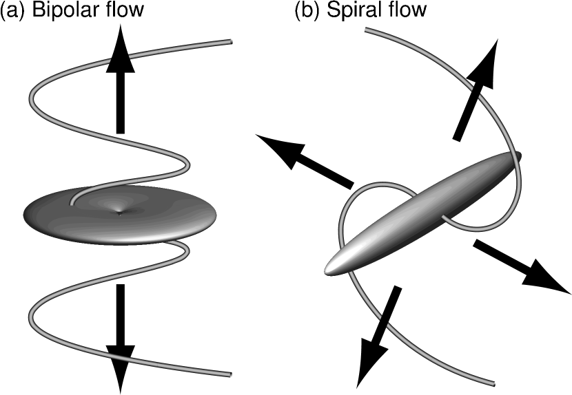
Figure 21.— Schematic diagram of two types of outflows: (a) bipolar flow and (b) spiral flow. The surfaces represent iso-density surfaces, the tubes denote the magnetic field lines. The arrows indicate the direction of the outflows.

The models here exhibit either bipolar or spiral outflows, as illustrated in Figure 21. The former has been produced in both aligned rotators (i.e., Tomisaka, 1998; Machida et al., 2004; Banerjee & Pudritz, 2006; Fromang et al., 2006) and inclined rotators (i.e., Matsumoto & Tomisaka, 2004; Hennebelle & Ciardi, 2009). The results of our simulations demonstrate that bipolar flows are also produced in turbulent cloud cores.

The bipolar flows are divided into two subtypes according to the configuration of the associated magnetic field. The outflows in the moderate field models have a poloidal magnetic field larger than the toroidal field, as shown in Figures 6b and 6d. Another subtype is reported in Figure 6a, where the toroidal magnetic field dominates over the poloidal field. The former outflow is driven by the magneto-centrifugal mechanism (c.f., Blandford & Payne, 1982; Pudritz & Norman, 1986), and the latter by the magnetic pressure gradient of the toroidal field component, categorized as I-type flow in Tomisaka (2002).

The spiral flow is a previously unreported type of outflow. The magnetic field lines are wound up by the rotation of the axes oriented perpendicular to the field. A similar magnetic field morphology was reported by Machida et al. (2006) for inclined rotators (see their Fig. 13). However, they did not confirm this type of outflow in their simulations because they could not follow the evolution for a sufficiently long period.

It is not yet known whether such spiral flows are stable over periods of more than several thousand years. When the angular momentum perpendicular to the magnetic field is released by the outflow, the outflow may transform from spiral to bipolar. In order to confirm this possibility, we need to employ the sink particle method to simulate longer timescales at a reasonable computational cost.

5.3. Probability of fragmentation

Figure 22.— Loci in the magnetic flux-spin relation plane for the models with ${\cal M}>0$. The abscissa and ordinate denote non-dimensional parameters of magnetic flux ($b$) and spin ($\omega$), respectively. Open circles, filled circles, and diamonds indicate the stages of $\rho=\rho_{0}$ (initial stage), $\rho_{\mathrm{cr}}$, and $\rho=10^{11}\rho_{0}$. Loci with continuous curves are for the isothermal phase ($\rho_{\mathrm{max}}\leq\rho_{\mathrm{cr}}$), and loci with dotted curves are for the adiabatic phase ($\rho_{\mathrm{max}}>\rho_{\mathrm{cr}}$). The quarter oval curve indicates the convergence curve, given by $(b/0.36)^{2}+(\omega/0.2)^{2}=1$.

Figure 22 displays the evolution of magnetic flux-spin relations for the models with ${\cal M}>0$. The magnetic flux-spin relations were proposed by Machida et al. (2005a, b) as a means of investigating fragmentation during cloud collapse. The abscissa and ordinate denote non-dimensional parameters of magnetic flux $b=|\bar{\mbox{\boldmath$B$}}|/(8\pi c_{p}^{2}\bar{\rho})^{1/2}$ and spin $\omega=|\bar{\mbox{\boldmath$\Omega$}}|/(4\pi G\bar{\rho})^{1/2}$, respectively, for the dense region with $\rho\geq 0.1\rho_{\mathrm{max}}$ (see Appendix C). This diagram predicts fragmentation driven by rotation.

The solid curves in Figure 22 are loci in the isothermal phase ($\rho_{\mathrm{max}}<\rho_{\mathrm{cr}}$) for all the turbulent models. Starting from the initial condition (open circles), all the loci drift in the $b-\omega$ plane, until they reach the convergence curve denoted by the black curve. This convergence was also seen for the case of collapse in the absence of turbulence (Machida et al., 2005a, b). They summarized the conditions for fragmentation as follows. If the locus reaches the horizontal part of the convergence curve (rotation dominant) during the isothermal collapse, the cloud core fragments. If it reaches the vertical part (magnetic field dominant), it does not. All the models examined here reach the vertical part of the convergence curve in the isothermal collapse phase, and they do not undergo fragmentation. This indicates that turbulent cloud cores have insufficient angular momentum to fragment.

Another possibility for fragmentation is turbulent fragmentation. In the massive models, the turbulence exceeds the thermal pressure as a supporting force against gravity. These models produce thin filaments. Each filament produces only one first core in the present simulations, because of the very small time steps in the adiabatic phase. However, the formed filaments are very thin and tend to undergo additional fragmentation in the later stages. Such fragmentation could be reproduced if sink particles were introduced into the simulations.

After the maximum density exceeds the critical density $\rho_{\mathrm{cr}}$, the loci traverse the convergence curve and they move in the leftward direction (dotted curves). This leftward movement is attributed to an increase in the sound speed $c_{p}$ in the adiabatic phase ($\rho_{\mathrm{max}}>\rho_{\mathrm{cr}}$). Some loci move close to the horizontal part of the convergence curve, where rotation support exceeds magnetic field support. Based on these models, a protoplanetary disk may fragment in the later stages if it is sufficiently massive compared to its central star.

6. Summary

The collapse of turbulent magnetized cloud cores is investigated by AMR simulations, resolving both the cloud core and the first core.

The cloud core has a complex density distribution in the low density region corresponding to its boundary with the parent cloud, because of disturbances due to turbulence. After the collapse begins, the density distribution becomes smooth in the collapsing region. This indicates that the collapse dilutes the tiny fluctuations caused by the turbulence. Even after formation of the first core, the edge of the cloud core remains turbulent.

The shape anisotropy of the collapsing region increases during isothermal collapse and depends mainly on the mass. When a cloud core is less massive ($f=1.68$), the dense region of the cloud core is oblate, with its minor axis parallel to the local magnetic field. The collapsing region is threaded by an hourglass-shaped distribution of magnetic field lines on a scale of $\lesssim 1000$ AU. When a cloud core is massive ($f=3.0$ and 6.0), the dense region of the cloud core is prolate, with the minor axis parallel to the local magnetic field. The extremely massive cloud ($f=6.0$) produces a very thin filament, which may later fragment.

In all cases, the orientation of the cloud core is controlled by the magnetic field. The minor axis of the collapsing region changes direction during the collapse, following the direction of the local magnetic field irrespective of the cloud core shape. Each model produces a spherical first core, in which the density is higher than $\simeq 10^{-10}\mathrm{g\,cm}^{-3}$. The first core is embedded in the infalling envelope.

The dependence of the shape on the mass can explained by the energy ratio between the thermal pressure and the turbulence. When the energy due to thermal pressure exceeds that due to turbulence, the cloud core becomes oblate in the early stages of collapse. If the opposite is the case, then the cloud core assumes a filamentary shape.

We found two types of outflows: bipolar and spiral flows. Bipolar flow is associated with the disk-shaped envelope, while the spiral flow is associated with the filamentary envelope. Bipolar flow tends to occur in less massive cloud cores, and the rotation axis, magnetic field, and the disk normal become aligned in the proximity of the first core. The disk-outflow system is inclined completely from the global magnetic field for the weak magnetized cloud core ($B=7\mu\mathrm{G}$). Even for the moderate field models ($B=19\mu\mathrm{G}$), the outflow direction diverges considerably from that of the global magnetic field by an angle of $\sim 40-50^{\circ}$. For the strong field model ($B=37\mu\mathrm{G}$), the disk envelope is aligned with its minor axis along the direction of the global magnetic field, while the outflow is not produced. The angular momentum perpendicular to the local magnetic field is selectively reduced in the dense region by magnetic braking and the outflow during the adiabatic phase in the bipolar flow models. The spiral flow tends to be associated with massive cloud cores, and the rotation axis is not aligned with the magnetic field in the envelope surrounding the first core.

Appendix A Energies of the critical Bonner-Ebert sphere

The gravitational potential $\Phi$ of the Bonner-Ebert sphere is obtained by solving the equations (see Chandrasekhar, 1939)

$$\frac{dw}{d\xi} = y$$ (A1)

$$\frac{dy}{d\xi} = -\frac{2y}{\xi}+e^{-w},$$ (A2)

imposing the boundary conditions of $w(0)=0$ and $y(0)=0$, where the non-dimensional variables $\xi$ and $w$ are defined by

$$\xi = \frac{r}{a},$$ (A3)

$$w = \frac{\Phi}{c_{s}^{2}}=-\ln\left(\frac{\rho}{\rho_{0}}\right),$$ (A4)

$$a = \left(\frac{c_{s}^{2}}{4\pi G\rho_{0}}\right)^{1/2}.$$ (A5)

The critical Bonner-Ebert sphere has a maximum radius of $\xi_{\mathrm{max}}=6.45$ ($r_{\mathrm{max}}=6.45a$). The central gravitational potential is equal to zero, $\Phi(0)=0$, owing to the boundary conditions. Considering an isolated critical Bonner-Ebert sphere, the gravitational potential in $r\leq r_{\mathrm{max}}$ is given by

$$\Psi(r)=\Phi(r)-\Phi(r_{\mathrm{max}})-G\frac{M(r_{\mathrm{max}})}{r_{\mathrm{max}}},$$ (A6)

where $M(\xi)$ denotes the mass inside the radius $\xi=r/a$,

$$M(\xi)=4\pi\int_{0}^{r}\rho r^{2}dr=4\pi a^{3}\rho_{0}y(\xi)\xi^{2}.$$ (A7)

The gravitational potential is therefore obtained as

$$\Psi(r)=c_{s}^{2}\left[w(\xi)-w(\xi_{\mathrm{max}})-\xi_{\mathrm{max}}y(\xi_{\mathrm{max}})\right].$$ (A8)

The gravitational energy is given by

$$E_{\mathrm{grav}} = \frac{1}{2}\int_{r\leq r_{\mathrm{max}}}\rho\Psi dV$$ (A9)

$$= 2\pi\rho_{0}c_{s}^{2}a^{3}\left\{\int_{0}^{\xi_{\mathrm{max}}}we^{-w}\xi^{2}d\xi-\left[\xi^{2}y(w+\xi y)\right]_{\xi=\xi_{\mathrm{max}}}\right\}$$ (A10)

$$= -352\rho_{0}c_{s}^{2}a^{3}$$ (A11)

The thermal energy is given by

$$E_{\mathrm{th}} = \frac{3}{2}\int_{r\leq r_{\mathrm{max}}}PdV$$ (A12)

$$= 6\pi a^{3}\rho_{0}c_{s}^{2}\left(y\xi^{2}\right)_{\xi=\xi_{\mathrm{max}}}$$ (A13)

$$= 296\rho_{0}c_{s}^{2}a^{3}.$$ (A14)

The magnetic field is expressed as $B=2\pi\alpha G^{1/2}\Sigma$ in our models, where the central surface density is given by

$$\Sigma = 2\int_{0}^{r_{\mathrm{max}}}\rho dr$$ (A15)

$$= 2\rho_{0}a\int_{0}^{\xi_{\mathrm{max}}}e^{-w}d\xi$$ (A16)

$$= 5.38\rho_{0}a.$$ (A17)

The magnetic energy is therefore given by

$$E_{\mathrm{mag}} = \int_{r\leq r_{\mathrm{max}}}\frac{B^{2}}{8\pi}dV$$ (A18)

$$= \frac{2\pi}{3}\rho_{0}c_{s}^{2}a^{3}\alpha^{2}\xi_{\mathrm{max}}^{3}\left(\int_{0}^{\xi_{\mathrm{max}}}e^{-w}d\xi\right)^{2}$$ (A19)

$$= 4061\alpha^{2}\rho_{0}c_{s}^{2}a^{3}.$$ (A20)

The kinetic energy is evaluated as

$$E_{\mathrm{kin}}=\frac{1}{2}\int_{r\leq r_{\mathrm{max}}}\rho\mbox{\boldmath$v$}^{2}dV.$$ (A21)

The initial velocity field is generated using a random number. When ten velocity fields are generated by changing the the seed of the random number, we obtained $E_{\mathrm{kin}}$ in the range of $(85.1-419)\rho_{0}c_{s}^{2}a^{3}{\cal M}^{2}$ and with an average of $220\rho_{0}c_{s}^{2}a^{3}{\cal M}^{2}$. For the velocity field used in this paper, the kinetic energy is evaluated as $E_{\mathrm{kin}}=139\rho_{0}c_{s}^{2}a^{3}{\cal M}^{2}$.

Introducing the parameters of the density enhancement factor $f$ (see equation [2]), we obtain scaling lows of $E_{\mathrm{th}}\propto f^{3/2}$, $E_{\mathrm{kin}}\propto f^{3/2}{\cal M}^{2}$, $E_{\mathrm{grav}}\propto f^{5/2}$, $E_{\mathrm{mag}}\propto f^{5/2}\alpha^{2}$, which yield energy ratios of $E_{\mathrm{th}}/|E_{\mathrm{grav}}|=0.836f^{-1}$, $E_{\mathrm{kin}}/|E_{\mathrm{grav}}|=0.394f^{-1}{\cal M}^{2}$, and $E_{\mathrm{mag}}/|E_{\mathrm{grav}}|=11.5\alpha^{2}$.

Appendix B Surface-to-volume ratio and axis ratios

In order to estimate the complexity of the density structure, the normalized surface-to-volume ratio is calculated. We calculate the surface and volume of a region $\Omega(\rho)$ where the density is larger than a given threshold $\rho$ and the point of maximum density is included. Based on Minkowski functional analysis, the volume $V(\rho)$ and surface $S(\rho)$ are calculated by

$$V(\rho) = N_{0}\Delta V,$$ (B1)

$$S(\rho) = (6N_{0}-2N_{1})\Delta S,$$ (B2)

$$N_{0} = \sum_{i,j,k}n_{i,j,k},$$ (B3)

$$N_{1} = \sum_{i,j,k}\left(n_{i,j,k}n_{i+1,j,k}+n_{i,j,k}n_{i,j+1,k}+n_{i,j,k}n_{i,j,k+1}\right),$$ (B4)

$$n_{i,j,k} = \left\{\begin{array}[]{ll}1&\mathrm{for\;a\;cell\;in\;}\Omega(\rho)\\ 0&\mathrm{otherwise}\end{array}\right.,$$ (B7)

where the subscripts $i,j,k$ denote the cell numbers in the $x$, $y$, and $z$-directions, respectively. The symbols $\Delta V$ and $\Delta S$ denote the volume and surface of a cell, respectively.

The surface-to-volume ratio $S(\rho)/V(\rho)^{2/3}$ has a large value when the region $\Omega(\rho)$ has a complex shape. The ratio $S(\rho)/V(\rho)^{2/3}$ has a minimum value when the region $\Omega(\rho)$ is spherical. We normalize the surface-to-volume ratio so that its value is unity for a sphere. Because the computational cell is cubic, the surface area of a sphere is given approximately by $6\pi r^{2}$ instead of $4\pi r^{2}$, where $r$ denotes the radius of the sphere. The volume of the sphere is approximated by $4\pi r^{3}/3$. The normalized surface-to-volume ratio is therefore given by

$$R(\rho)=\frac{2^{4/3}}{3^{2/3}6\pi^{1/3}}\frac{S(\rho)}{V(\rho)^{2/3}}=0.138\frac{S(\rho)}{V(\rho)^{2/3}}.$$ (B8)

We also measure the lengths of the principal axes of the region $\Omega(\rho)$, calculating the moment of the coordinates

$$K_{\hat{i},\hat{j}}=\frac{1}{V(\rho)}\sum_{i,j,k}n_{i,j,k}(r_{i,j,k,\hat{i}}-r_{g,\hat{i}})(r_{i,j,k,\hat{j}}-r_{g,\hat{j}})\Delta V,$$ (B9)

where $\mbox{\boldmath$r$}_{i,j,k}=(r_{i,j,k,1},r_{i,j,k,2},r_{i,j,k,3})=(x_{i,j,k},y_{i,j,k},z_{i,j,k})$ represents the coordinates of the cell. The coordinates of the baricenter $\mbox{\boldmath$r$}_{g}$ are estimated by

$$\mbox{\boldmath$r$}_{g}=\frac{1}{V(\rho)}\sum_{i,j,k}n_{i,j,k}\mbox{\boldmath$r$}_{i,j,k}\Delta V.$$ (B10)

The three principal axes $a_{n}$ are defined by the square roots of three eigenvalues of $K_{\hat{i},\hat{j}}$, arranged in ascending order ($a_{1}<a_{2}<a_{3}$). The axis ratios are estimated as $a_{2}/a_{1}$ and $a_{3}/a_{1}$.

When the region $\Omega$ overlaps the boundary of the computational domain, care must be taken regarding the periodic boundary conditions. Moreover, the axis ratios are obtained only when the one-dimensional length of the region $\Omega$ is smaller than the width of the computational domain.

Appendix C Analysis of dense region

We calculate the mean values of the dense region of the cloud cores, $\bar{\rho}$, $\bar{\mbox{\boldmath$B$}}$, $J$, $\bar{\mbox{\boldmath$\Omega$}}$, and the direction of the minor axis. The mean density of the dense region is defined by $\bar{\rho}=M/V$, where

$$M=\int_{\rho\geq 0.1\rho_{\mathrm{max}}}\rho(\mbox{\boldmath$r$})dV,$$ (C1)

and

$$V=\int_{\rho\geq 0.1\rho_{\mathrm{max}}}dV.$$ (C2)

The integral $\int_{\rho\geq 0.1\rho_{\mathrm{max}}}dV$ denotes a volume integral over the region with $\rho\geq 0.1\rho_{\mathrm{max}}$. The mean magnetic field in the dense region is defined by

$$\bar{\mbox{\boldmath$B$}}=\frac{1}{V}\int_{\rho\geq 0.1\rho_{\mathrm{max}}}\mbox{\boldmath$B$}(\mbox{\boldmath$r$})dV.$$ (C3)

The angular momentum in the dense region is defined by

$$\mbox{\boldmath$J$}=\int_{\rho\geq 0.1\rho_{\mathrm{max}}}(\mbox{\boldmath$r$}-\mbox{\boldmath$r$}_{g})\times\left[\mbox{\boldmath$v$}(\mbox{\boldmath$r$})-\mbox{\boldmath$v$}_{g}\right]\rho(\mbox{\boldmath$r$})dV,$$ (C4)

where $\mbox{\boldmath$r$}_{g}$ and $\mbox{\boldmath$v$}_{g}$ denote the coordinates and velocity of the baricenter, estimated respectively as

$$\mbox{\boldmath$r$}_{g}=\frac{1}{M}\int_{\rho\geq 0.1\rho_{\mathrm{max}}}\mbox{\boldmath$r$}\rho(\mbox{\boldmath$r$})dV,$$ (C5)

and

$$\mbox{\boldmath$v$}_{g}=\frac{1}{M}\int_{\rho\geq 0.1\rho_{\mathrm{max}}}\mbox{\boldmath$v$}(\mbox{\boldmath$r$})\rho(\mbox{\boldmath$r$})dV.$$ (C6)

The mean angular velocity in the dense region is defined by

$$\bar{\mbox{\boldmath$\Omega$}}=\bar{\mbox{\boldmath$I$}}^{-1}\mbox{\boldmath$J$},$$ (C7)

where $\bar{\mbox{\boldmath$I$}}$ indicates the moment of inertia, of which the components are estimated as

$$\bar{I}_{ij}=\int_{\rho\geq 0.1\rho_{\mathrm{max}}}\left[(\mbox{\boldmath$r$}-\mbox{\boldmath$r$}_{g})^{2}\delta_{ij}-(r_{i}-r_{g,i})(r_{j}-r_{g,j})\right]\rho(\mbox{\boldmath$r$})dV,$$ (C8)

and the subscripts $i$, $j$ represent coordinate labels, i.e., $x=r_{1}$, $y=r_{2}$, $z=r_{3}$, and $\delta_{ij}$ denotes the Kronecker delta.

The axes of the dense region are derived from the moment of the coordinates,

$$\bar{K}_{i,j}=\int_{\rho\geq 0.1\rho_{\mathrm{max}}}(r_{i}-r_{g,i})(r_{j}-r_{g,j})\rho(\mbox{\boldmath$r$})dV.$$ (C9)

The eigenvectors of $\bar{K}_{i,j}$ indicate the orientation of the principal axes.

The velocity dispersion is given by

$$\left<\Delta v\right>=\left\{\frac{1}{M}\int_{\rho\geq 0.1\rho_{\mathrm{max}}}\left[\mbox{\boldmath$v$}(\mbox{\boldmath$r$})-\mbox{\boldmath$v$}_{g}\right]^{2}\rho(\mbox{\boldmath$r$})dV\right\}^{1/2}.$$ (C10)

The velocity dispersion for the radial velocity is also estimated as

$$\left<\Delta v_{r}\right>=\left[\frac{1}{M}\int_{\rho\geq 0.1\rho_{\mathrm{max}}}v_{r}(\mbox{\boldmath$r$})^{2}\rho(\mbox{\boldmath$r$})dV\right]^{1/2},$$ (C11)

where $v_{r}(\mbox{\boldmath$r$})$ denotes the radial component of the relative velocity, $\mbox{\boldmath$v$}(\mbox{\boldmath$r$})-\mbox{\boldmath$v$}_{g}$, with respective to the position of the baricenter, $\mbox{\boldmath$r$}_{g}$.

References

- Banerjee & Pudritz (2006) Banerjee, R., & Pudritz, R. E. 2006, ApJ, 641, 949
- Bate (2009) Bate, M. R. 2009, MNRAS, 397, 232
- Blandford & Payne (1982) Blandford, R. D., & Payne, D. G. 1982, MNRAS, 199, 883
- Bonnor (1956) Bonnor, W. B. 1956, MNRAS, 116,351
- Burkert & Bodenheimer (2000) Burkert, A., & Bodenheimer, P. 2000, ApJ, 543, 822
- Chandrasekhar (1939) Chandrasekhar, S. 1939, Chicago, Ill., The University of Chicago press [1939],
- Commerçon et al. (2010) Commerçon, B., Hennebelle, P., Audit, E., Chabrier, G., & Teyssier, R. 2010, A&A, 510, L3
- Crutcher (1999) Crutcher, R. M. 1999, ApJ, 520, 706
- Dedner et al. (2002) Dedner, A., Kemm, F., Kröner, D., Munz, C.-D., Schnitzer, T., & Wesenberg, M. 2002, Journal of Computational Physics, 175, 645
- Dubinski et al. (1995) Dubinski, J., Narayan, R., & Phillips, T. G. 1995, ApJ, 448, 226
- Ebert (1955) Ebert, R. 1955, Z. Astrophys., 37, 222
- Fromang et al. (2006) Fromang, S., Hennebelle, P., & Teyssier, R. 2006, A&A, 457, 371
- Gammie et al. (2003) Gammie, C. F., Lin, Y.-T., Stone, J. M., & Ostriker, E. C. 2003, ApJ, 592, 203
- Girart et al. (2006) Girart, J. M., Rao, R., & Marrone, D. P. 2006, Science, 313, 812
- Goodwin et al. (2004) Goodwin, S. P., Whitworth, A. P., & Ward-Thompson, D. 2004, A&A, 414, 633
- Goodman et al. (1998) Goodman, A. A., Barranco, J. A., Wilner, D. J., & Heyer, M. H. 1998, ApJ, 504, 223
- Hennebelle & Ciardi (2009) Hennebelle, P., & Ciardi, A. 2009, A&A, 506, L29
- Henning et al. (2001) Henning, T., Wolf, S., Launhardt, R., & Waters, R. 2001, ApJ, 561, 871
- Jijina et al. (1999) Jijina, J., Myers, P. C., & Adams, F. C. 1999, ApJS, 125, 161
- Klein et al. (2007) Klein, R. I., Inutsuka, S.-I., Padoan, P., & Tomisaka, K. 2007, Protostars and Planets V, 99
- Langer et al. (1995) Langer, W. D., Velusamy, T., Kuiper, T. B. H., Levin, S., Olsen, E., & Migenes, V. 1995, ApJ, 453, 293
- Larson (1969) Larson, R. B. 1969, MNRAS, 145, 271
- Larson (1981) Larson, R. B. 1981, MNRAS, 194, 809
- Li et al. (2004) Li, P. S., Norman, M. L., Mac Low, M.-M., & Heitsch, F. 2004, ApJ, 605, 800
- Lin et al. (1965) Lin, C. C., Mestel, L., & Shu, F. H. 1965, ApJ, 142, 1431
- Machida et al. (2004) Machida, M. N., Tomisaka, K., & Matsumoto, T. 2004, MNRAS, 348, L1
- Machida et al. (2005a) Machida, M. N., Matsumoto, T., Tomisaka, K., & Hanawa, T. 2005, MNRAS, 362, 369
- Machida et al. (2005b) Machida, M. N.,Matsumoto, T., Hanawa, T., & Tomisaka, K. 2005, MNRAS, 362, 382
- Machida et al. (2006) Machida, M. N., Matsumoto, T., Hanawa, T., & Tomisaka, K. 2006, ApJ, 645, 1227
- Masunaga, Miyama, & Inutsuka (1998) Masunaga, H., Miyama, S. M., & Inutsuka, S. 1998, ApJ, 495, 346.
- Matsumoto & Tomisaka (2004) Matsumoto, T., & Tomisaka, K. 2004, ApJ, 616, 266
- Matsumoto et al. (1997) Matsumoto, T., Hanawa, T., & Nakamura, F. 1997, ApJ, 478, 569
- Matsumoto (2007) Matsumoto, T. 2007, PASJ, 59, 905
- McKee & Ostriker (2007) McKee, C. F., & Ostriker, E. C. 2007, ARA&A, 45, 565
- Mellon & Li (2008) Mellon, R. R., & Li, Z.-Y. 2008, ApJ, 681, 1356
- Mellon & Li (2009) Mellon, R. R., & Li, Z.-Y. 2009, ApJ, 698, 922
- Myers et al. (1991) Myers, P. C., Fuller, G. A., Goodman, A. A., & Benson, P. J. 1991, ApJ, 376, 561
- Nakamura & Li (2008) Nakamura, F., & Li, Z.-Y. 2008, ApJ, 687, 354
- Nakano & Nakamura (1978) Nakano, T., & Nakamura, T. 1978, PASJ, 30, 671
- Offner & Krumholz (2009) Offner, S. S. R., & Krumholz, M. R. 2009, ApJ, 693, 914
- Offner et al. (2008) Offner, S. S. R., Klein, R. I., & McKee, C. F. 2008, ApJ, 686, 1174
- Price & Bate (2008) Price, D. J., & Bate, M. R. 2008, MNRAS, 385, 1820
- Pudritz & Norman (1986) Pudritz, R. E., & Norman, C. A. 1986, ApJ, 301, 571
- Ryden (1996) Ryden, B. S. 1996, ApJ, 471, 822
- Shu & Li (1997) Shu, F. H., & Li, Z.-Y. 1997, ApJ, 475, 251
- Schleuning (1998) Schleuning, D. A. 1998, ApJ, 493, 811
- Sugitani et al. (2010) Sugitani, K., et al. 2010, ApJ, 716, 299
- Tafalla et al. (2002) Tafalla, M., Myers, P. C., Caselli, P., Walmsley, C. M., & Comito, C. 2002, ApJ, 569, 815
- Tomida et al. (2010) Tomida, K., Tomisaka, K., Matsumoto, T., Ohsuga, K., Machida, M. N., & Saigo, K. 2010, ApJ, 714, L58
- Tomisaka et al. (1988) Tomisaka, K., Ikeuchi, S., & Nakamura, T. 1988, ApJ, 335, 239
- Tomisaka (1998) Tomisaka, K. 1998, ApJ, 502, L163
- Tomisaka (2002) Tomisaka, K. 2002, ApJ, 575, 306
- Truelove et al. (1997) Truelove, J. K., Klein, R. I., McKee, C. F., Holliman, J. H., II, Howell, L. H., & Greenough, J. A. 1997, ApJ, 489, L179
- Vallée et al. (2003) Vallée, J. P., Greaves, J. S., & Fiege, J. D. 2003, ApJ, 588, 910
- Wang et al. (2010) Wang, P., Li, Z.-Y., Abel, T., & Nakamura, F. 2010, ApJ, 709, 27
- Wolf et al. (2003) Wolf, S., Launhardt, R., & Henning, T. 2003, ApJ, 592, 233
- Zuckerman & Evans (1974) Zuckerman, B., & Evans, N. J., II 1974, ApJ, 192, L149