The Origin and Evolution of the Mass-Metallicity Relation at High Redshift using GalICS

Abstract

The GalICS (Galaxies in Cosmological Simulations) semi-analytical model of hierarchical galaxy formation is used to investigate the effects of different galactic properties, including star formation rate (SFR) and outflows, on the shape of the mass metallicity relation and to predict the relation for galaxies at redshift $z=2.27$ and $z=3.54$. Our version of GalICS has the chemical evolution implemented in great detail and is less heavily reliant on approximations such as instantaneous recycling. We vary the model parameters controlling both the efficiency and redshift dependence of the SFR as well as the efficiency of supernova feedback. We find that the factors controlling the SFR influence the relation significantly at all redshifts and require a strong redshift dependence, proportional to $1+z$, in order to reproduce the observed relation at the low mass end. Indeed, at any redshift, the predicted relation flattens out at the high mass end resulting in a poorer agreement with observations in this regime. We also find that variation of the parameters associated with outflows has a minimal effect on the relation at high redshift but does serve to alter its shape in the more recent past. We thus conclude that the relation is one between SFR and mass and that outflows are only important in shaping the relation at late times. When the relation is stratified by SFR it is apparent that the predicted galaxies with increasing stellar masses have higher SFRs, supporting the view that galaxy downsizing is the origin of the relation. Attempting to reproduce the observed relation, we vary the parameters controlling the efficiency of star formation and its redshift dependence and compare the predicted relations with Erb et al. (2006) at $z=2.27$ and Maiolino et al. (2008) at $z=3.54$ in order to find the best-fitting parameters. We succeed in fitting the relation at $z=3.54$ reasonably well, however we fail at $z=2.27$, our relation lying on average below the observed one at the one standard deviation level. We do, however, predict the observed evolution between $z=3.54$ and $z=0$. Finally, we discuss the reasons for the above failure and the flattening at high masses, with regards to both the comparability of our predictions with observations and the possible lack of underlying physics. Several of these problems are common to many semi-analytic/hybrid models and so we discuss possible improvements and set the stage for future work by considering how the predictions and physics in these models can be made more robust in light of our results.

1 Introduction

The existence of a relation between luminosity (or mass) and metallicity in irregular and blue compact galaxies was first proposed by Lequeux et al. (1979) and later confirmed by Skillman et al. (1989). Garnett & Shields (1987) extended the relation to spiral galaxies. Recently Tremonti et al. (2004) examined the relation at $z\!\approx\!0$ using $\sim$53000 local star-forming galaxies in the SDSS and found that $12+\log(O/H)$ increases steeply for $10^{8.5}<M_{\star}/M_{\odot}<10^{10.5}$ but flattens at larger masses.

Several explanations for such a relation have been put forward. For instance, Tremonti et al. (2004) suggest that galaxies form similar fractions of stars independent of their mass. Less massive galaxies are simply less efficient at retaining gas due to their shallower potential wells and lose newly produced metals to galactic outflows. Another possibility (Maiolino et al., 2008) is that more massive galaxies had higher specific star formation rates (SFR per unit stellar mass) or a higher star formation efficiency (SFR per unit gas mass) in the past so form a larger fraction of stars in the same Hubble time. In this case the higher metallicity is due to the conversion of a larger amount of primordial gas into C, N and O. This scenario is known as galaxy down-sizing for which there is a plethora of observational evidence (e.g Pérez-González et al. (2008)). An alternate explanation (Köppen et al., 2007) is a variation in the initial mass function (IMF) in different star forming environments. It is not known at present which process is responsible for the ubiquitously observed relation however it is likely that all three contribute to some extent. Interestingly, a similar relation holds for the stars of gas-poor galaxies (Faber, 1973; Brodie & Huchra, 1991).

A lot of effort has been made to understand whether an underlying common physical origin for the above mentioned relation exists, as well as to determine the highest redshift at which the mass-metallicity relation holds. Erb et al. (2006) have measured the relation at $z\approx 2.27$ using the [NII]/H$\alpha$ ratio in stacked spectra for a sample of 87 rest-frame ultraviolet-selected star-forming galaxies. Recently, Maiolino et al. (2008) have used deep near-IR spectroscopy of H$\beta$ and [OIII]5007 shifted into the K band as well as [OII]3727 and [NeIII]2870 shifted into the H band to measure the relation for nine star forming galaxies at $z\sim 3.54$. More recently, Mannucci et al. (2009) have used near-IR spectroscopy of the optical lines [OII]$\lambda$3727, H$\beta$, and [OIII]$\lambda$5007 for a sample of 10 Lyman-break galaxies (LGBs) at $z\sim 3$ to derive their SFR, metallicity, gas fraction and effective yield. Using optical, near- IR and Spitzer/IRAC photometry, they have measured the stellar mass of each galaxy in order to guarantee a robust estimate of the mass-metallicity relation. Finally, Mannucci et al. (2010) introduce the SFR-mass-metallicity relation and show that it does not evolve with redshift up to $z\sim 2$. They argue that the apparent evolution of the mass-metallicity relation inferred by past works at redshifts below $z\sim 2$ is only due to selection effects, where independent surveys sample different areas of the SFR-mass-metallicity “surface” at different redshifts (in particular those with a higher SFR at higher redshifts). A strong evolution still occurs for $z>2$.

Previous attempts at modelling hierarchical galaxy evolution through semi-analytic models and $N$-body simulations have shown that a mass-metallicity relation is predicted also in the hierarchical scenario (De Rossi et al., 2007). In one such simulation De Rossi et al. (2007) predicted the relation over the redshift range $0\leq z\leq 3$; however the predicted metallicities are always larger than the observed ones. The authors attribute this to the lack of supernova feedback in the model and thus the lack of outflows from the galaxies. De Lucia et al. (2004) predicts a relation at $z\approx 0$ for three models characterized by different feedback processes. It was found that all three models predict galaxies whose average metallicities lie within one standard deviation of the median mass-metallicity relation observed by Tremonti et al. (2004), at variance with the results of Finlator & Davé (2008), who found that the predicted relation depends strongly on the galactic outflow model used. They also found that a lack of outflows lead to galaxies that were too enriched in metals, consistent with the results of De Rossi et al. (2007). According to Finlator & Davé (2008) only a model where the wind was momentum driven could reproduce the observed relation (Erb et al., 2006). In this simulation the relation was reproduced reasonably well within experimental uncertainties and could match the observed relation in slope, amplitude and scatter. By incorporating mass dependent galactic winds into the parallel tree-SPH code GADGET-2 (Springel, 2005), Kobayashi et al. (2007) predicted a relation at $z\approx 2$ that is consistent with the observations of Erb et al. (2006) for massive galaxies only. Their predictions exhibit a significant scatter and their model suffers from the fact that it does not predict the termination of star formation in massive galaxies at late times. Finally, using $N$-body/hydrodynamical simulations Mouchine et al. (2008) were able to reproduce the observed relations over the range $0\leq z\leq 1.2$ with minimal scatter although at higher redshifts the simulated relation predicts galaxies with higher metallicities than are observed (Erb et al., 2006).

As noted in Maiolino et al. (2008), where we address the reader for a more extended discussion of the single cases, many of the above mentioned attempts have failed to reproduce the observed relation at $z\sim 3$. Calura et al. (2009) have recently been successful in predicting the relation over the range $0.07\leq z\leq 3.54$ using a chemical evolution model that predicts the relation separately for galaxies of different morphological type. Rather than collectively fitting the relation they have found that the relation at low redshifts is best fit by considering only spiral and irregular galaxies whilst at intermediate redshifts ($z\sim 2$) the relation is best fit by a mixture of proto-spirals and proto-ellipticals. At $z=3.54$ they predict that the relation is best fit by proto-ellipticals alone. In this work we attempt to reproduce and explain the observed relation at $z=2.27$ and $z=3.54$ by testing aspects of the galactic outflows (in common with many of the above models) as well as other methods including different IMFs and a redshift dependent SFR. In order to do this, we make use of an up-to-date version of GalICS in which a detailed treatment of the chemical evolution has been implemented; details of which can be found in Pipino et al. (2009). This model - which tracks the evolution of H, He, O and Fe - has the chemical evolution implemented in great detail. It does not rely on the instantaneous recycling approximation but instead uses a self-consistent prescription for both type Ia and Type II supernovae ejecta, which includes the effects of finite stellar lifetimes. We consider this aspect the main innovation of our approach.

We assume a flat (critical density) lambda cold dark matter cosmology ($\Lambda$CDM) with cosmological parameters taken from the WMAP three year results (WMAP3) (Spergel et al., 2007). These are $\Omega_{0}=0.24$, $\Omega_{\Lambda}=0.76$, $h=0.73$ and $\Omega_{B}=0.06h$ where all the symbols have their usual meaning.

In section 2 we describe the GalICS model and introduce the free parameters that it uses to control the star formation efficiency, redshift dependence of the SFR, supernova feedback and the efficiency with which gas that was once ejected by the galaxy is re-accreted. In section 3 we show the data with which we compare our predictions and discuss their uncertainties, mainly due to calibration issues. In section 4 we determine the effect of varying the free parameters and IMF upon the predicted relation and compare our predictions with observations. In section 5 we then present the results of using the best-fitting parameters for the entire population of model galaxies and interpret the results physically. In section 6 we draw our conclusions.

2 The GalICS Model

GalICS is a semi analytic hybrid model of hierarchial galaxy formation that combines the output of large $N$-body cosmological simulations to track the evolution of baryonic matter in galaxies through their dark matter haloes. The evolution of galaxies is tracked using halo merging trees that follow the hierarchial evolution of small objects at early times that may or may not develop into larger ones through merging processes or accretion of matter (Hatton et al., 2003). GalICS assigns a morphology to a galaxy instantly after a merger based on the ratio of the bulge to disc B-band luminosities. In outline, as hot gas cools and falls into the centre of its dark matter halo, it settles in a rotationally supported disc. The galaxies remain pure discs if their disc is globally stable and they do not undergo a merger with another galaxy. In the case where a significant merger occurs, we employ a recipe to distribute the stars and gas in the galaxy between three different components in the resulting, post-merger galaxy, the disc, the bulge, and a star-burst (see Hatton et al., 2003). In the case of a disc instability, we simply transfer the mass of the gas and stars necessary to make the disc stable to the burst component, and compute the properties of the bulge/burst in a similar fashion to that described in Hatton et al. (2003). The star-burst scale is $r_{\textrm{burst}}=0.1r_{\textrm{bulge}}$, so that the characteristic timescale for the star formation is shorter than in the bulge, hence leading to a faster consumption of the gas. The star formation rates are even higher than those in the discs, but have an instantaneous duration. The burst stellar population becomes part of the bulge stellar population when the stars have reached an age of 100 Myr. Since we will only be using the model predictions for high redshift it does not make sense to classify the galaxies by local ($z=0$) standards and so here we consider all of the predicted galaxies no matter the GalICS assigned morphology.

The simulation models the universe as a box of comoving length of $150$ Mpc. Like any numerical simulation, GalICS has a finite baryonic mass resolution. The minimum baryonic mass that we consider resolved in this simulation is $2\textrm{x}10^{9}M_{\odot}$, which is a factor of ten lower than the fiducial GalICS value (Hatton et al. 2003). The baryonic gas in galaxies is initially primordial comprising of Hydrogen and Helium. The metal content increases as time passes due to the synthesis of these elements in stars during their lifetime and their subsequent release into the inter-stellar medium (ISM) upon the stars death. A detailed description of the entire GalICS model may be found in Hatton et al. (2003) and an updated version (as far as the implementation of the chemical evolution of O and Fe is concerned) of the model that we use in this paper can be found in Pipino et al. (2009).

The main novelty of the present version of GalICS (Pipino et al., 2009) is the implementation of a self-consistent treatment of the chemical evolution with finite stellar lifetimes and both type Ia (SNIa) and type II (SNII) supernovae ejecta. In practice, we follow the chemical evolution of only four elements, namely H, He, O and Fe. This set of elements is good enough to characterize our simulated galaxies from the chemical evolution point of view as well as small enough in order to minimize computational resources. Also, the reader should remember that O is the major contributor to the total metallicity.

We adopt the yields from Iwamoto et al. (1999) and references therein for both SNIa and SNII. The reader should note that a change in the stellar yields will introduce a systematic offset of a few tenths of a dex in the model predictions (see Thomas et al., 2007; Pipino & Matteucci, 2004), hence it might leave room for some fine-tuning for a suitable choice of stellar nucleosynthesis. However, being only an offset, this change cannot create nor modify the slope of the predicted relations. But, most importantly, the successful calibration of our model with element ratios observed in Milky Way stars (see Pipino et al., 2009) does not allow significant modifications of the underlying stellar yields.

The SNIa rate for a simple stellar population (SSP) formed at a given time is calculated assuming the single degenerate scenario and the Matteucci & Recchi (2001) Delay Time Distribution (DTD). The convolution of this DTD with the SFR (see Greggio, 2005) gives the total SNIa rate.

Stars - and baryonic processes at the galactic scale that need finer detail - are evolved between time-steps using sub-stepping of at least 1 Myr. During each sub-step, stars release mass and energy into the interstellar medium. In GalICS, the enriched material released in the late stages of stellar evolution is mixed to the cold phase, while the energy released from supernovae is used to re-heat the cold gas and return it to the hot phase in the halo. The rate of mass loss in the supernova-driven wind that flows out of the disc is directly proportional to the supernova rate (see below).

Throughout this work, we assume chemical homogeneity (instantaneous mixing), such that outflows caused by feedback processes are assumed to have the same metallicity as the inter-stellar medium, though in reality the situation cannot be captured by our simple recipe (Strickland & Heckman, 2009) and newly produced metals are more likely to be ejected than the gas (see, for example, Recchi et al., 2004) . Note that, due to the fine sub-stepping used for the stellar evolution, ejecta from SNII and the contributions of single low-mass stars is implemented without the need to assume the instantaneous recycling approximation.

Below we focus on the main free parameters of the model that we will change in order to study the build-up of the mass-metallicity relation. A complete, detailed description of GalICS and a compendium of its entire features may be found in Hatton et al. (2003).

2.1 Initial Mass Function

We use the Salpeter (Salpeter, 1955) IMF

$$\phi\!\left(m\right)\propto m^{-2.35}$$ (1)

in our simulations. The effect of changing the IMF is then investigated by replacing it with the Kennicutt (Kennicutt et al., 1994) IMF,

$$\phi\!\left(m\right)\propto\left\{\begin{array}[]{l l}m^{-1.4}\,,&\quad\mbox{$m<1M_{\odot}$}\\ m^{-2.5}\,,&\quad\mbox{otherwise}\\ \end{array}\right.\,,$$ (2)

in section 4. We take as the mass range $0.1\leq m\leq 40M_{\odot}$ for each IMF which determines the normalisation. This is lower than adopted ($65M_{\odot}$) by Maiolino et al. (2008); whose value would result in a higher O abundance on average of less than $0.1$ dex. We note here that an even higher cutoff (greater than $80M_{\odot}$) would lead to a change in the predicted O abundance of less than 0.3 dex, although we must rely on the extrapolation of the nucleosynthetic yields available in the literature, whereas the mass range $m<40M_{\odot}$ is where the O yields are more robust. We have performed tests that show, as expected, that changes in the yields effect only the normalization of the Mass-metallicity relation and not the slope. We therefore prefer to keep the same configuration as Pipino et al. (2009), where the chemical evolution scheme (with a $40M_{\odot}$ upper limit) has been calibrated on observations of the Milky Way. Moreover, there are indications (Cescutti & Chiappini, 2010) that O production decreases with metallicity due to metal-dependent mass loss. In light of the above caveats, the reader should keep in mind that some fine-tuning of the normalization in the predicted mass-metallicity relation could be performed by acting on either the IMF or the O yields.

2.2 Star Formation

The star formation rate is given by

$$\noindent\textrm{SFR}=\alpha\frac{M_{\textrm{cold}}}{t_{\textrm{dyn}}}\left(1+z\right)^{\beta}\,,$$ (3)

where $M_{\textrm{cold}}$ is the mass of cold gas. The dynamical timescale $t_{\textrm{dyn}}$ is defined as the time taken for matter at the half-mass radius to reach either the opposite side of the galaxy (disc) or the centre of the galaxy (bulge) and is given in Hatton et al. (2003). The free parameter $\alpha$ sets the efficiency of star formation and $\beta$ controls its redshift (time) dependence (if any). TheGalICS fiducial value of $\alpha$ (Hatton et al., 2003) is $0.02$ after Guiderdoni et al. (1998) and others (see Somerville & Primack (1999) tables 4 and 5) have used values in the range $0.01\leq\alpha\leq 0.25$ with GalICS restricted to the range $0.01\leq\alpha\leq 0.1$ (Hatton et al., 2003). In this work we vary $\alpha$ over the range $0.01\leq\alpha\leq 0.05$. There is observational evidence that the SFR was higher in the past (Lilly et al., 1996; Spergel et al., 1997; Helmboldt et al., 2004; Juneau et al., 2005; Feulner et al., 2005) and so we focus on positive values of $\beta$. Currently there is no ubiquitously accepted theoretical explanation for this. One possibility is that the cosmic expansion means that galaxies were closer together in the past and could thus interact more easily than at later times giving a higher merger rate than at present. There is, however, evidence that the number of star-forming galaxies at $z\approx 2$ is much higher than the predicted number of mergers (Conroy et al., 2008) indicating that much of the star formation is not merger driven. Some (Pipino et al., 2009) argue that positive feedback from the central super-massive black hole during its early growth period can account for these observations and others that larger galaxies (that would have formed initially) have an overall higher cross section per unit mass (Ferreras & Silk, 2003) and thus accrete gas faster than smaller galaxies formed more recently. Successfully simulating a predicted mass-metallicity relation that closely matches the observed one may elucidate the mechanism by which galaxies have a higher SFR in the past. The GalICS fiducial value of $\beta$ is $0$, however, using $\beta=0.6$ in order to incorporate the effect of rapid accretion by cold flows, Cattaneo et al. (2006) have managed to improve the fitting of the GalICS predicted luminosity function of Lyman-break galaxies to observations. Hence, we vary $\beta$ around this value. In section 5 we will discuss our predicted star formation rates in comparison with those that are observed in the galaxy samples with which we compare our predicted mass-metallicity relations.

2.3 Supernova Feedback

Massive stars will become type-II supernovae that release energy into the ISM causing a fraction of the gas to be ejected. If the energy is sufficient this ejected gas may leave the galaxy inhibiting star formation. This process is known as supernova feedback. We model the outflow rate using the formula from Silk (2003)

$$\dot{m}=2\varepsilon\frac{E_{\textrm{SN}}\eta_{\textrm{SN}}}{v_{\textrm{esc}}^{2}}\textrm{SFR}\,.$$ (4)

where SFR is given in equation 3. Here $\eta_{\textrm{SN}}$ is the number supernovae per unit star forming mass, which we take as $7.4\textrm{x}10^{-3}$/$M_{\odot}$ and $E_{\textrm{SN}}$ is the energy released by a single supernova assumed to have a constant value of $10^{44}$J. The escape velocity $v_{\textrm{esc}}$ is given separately for bulges, discs and haloes in GalICS I (Hatton et al., 2003). The free parameter $\varepsilon$ determines the efficiency at which gas from supernovae is injected into the ISM. The mass-loading factor is then equal to the factors pre-multiplying the SFR and hence $\varepsilon^{-1}$ can be though of as the efficiency of mass-loading. The GalICS fiducial value is $0.3$ and others have used values in the range $0.05\leq\varepsilon\leq 0.2$ (see Somerville & Primack (1999) tables 4 and 5). Cattaneo et al. (2006) have found that $\varepsilon=0.2$ is the best-fitting value if GalICS is used to predict the luminosity function of Lyman-break galaxies. Hence, we initially vary $\varepsilon$ in the range $0\leq\varepsilon\leq 0.3$.

2.4 Ejection of Matter from the Halo

Type-II supernova and other galaxy forming processes may lead to the ejection of gas and metals from the halo. These individual processes are difficult to model (Hatton et al., 2003) and the GalICS model accommodates them by storing all ejected gas and metals ejected from the halo in a ‘reservoir’ from which they may or may not be re-accreted at a later time. When matter is accreted from extra galactic sources a certain fraction is primordial and the rest is drawn from the reservoir. The efficiency of re-accretion from the reservoir is characterized by the parameter $\zeta$, the halo recycling efficiency. If $\zeta=0$ then material ejected from the halo is lost permanently. If $\zeta=1$ then all matter accreted is drawn from the reservoir until it is depleted at which point any further gas accreted is assumed primordial. Recently, Oppenheimer et al. (2009) have studied the effects of recycling on the SFRs and stellar mass function of galaxies in cosmological hydrodynamical simulations and have found that it is the dominant factor in galaxy growth at $z\leq 1$, ejecta being the important factor at $z\geq 2$. Hence, in this work we focus on the supernova feedback efficiency and do not vary $\zeta$, holding it constant at the GalICS fiducial value, $0.3$, so that during any gas re-accretion process, 30% is drawn from the reservoir (provided it is not depleted), the remainder being of primordial metallicity.

3 Data

The gas metallicity must be determined using strong line metallicity diagnostics (Maiolino et al., 2008) which relies on the fact that the ratio of various strong optical emission lines depend upon the gas metallicity in a known manner. Thus these ratios must be calibrated against metallicity. Calibrations have only been performed in narrow metallicity ranges. These calibrations are often inconsistent with each other and can lead to different metallicity offsets of up to $0.7$ dex and the difference in the shape of the curve is often large (Kewley & Ellison, 2008). Since data measured at different redshifts may be measured using different optical lines it is essential to ensure a correct intercalibration between the data fits so that the correct evolution of the relation can be seen. These intercalibration issues are tackled by Nagao et al. (2006) and by Maiolino et al. (2008), who take a large sample of local galaxies spanning a wide range of metallicities ($7.2<12+\log(O/H)<9.2$, accurately measured by using both the electron temperature method and photoinoization models) and cross-calibrate the various strong line ratio diagnostics on the same metallicity scale.

We take as our observed trend the AMAZE (Maiolino et al., 2008) mass-metallicity relation

$$12+\log\left(O/H\right)=-0.0864\left(\log M_{\star}-\log M_{\mathrm{0}}\right)^{2}+K_{\mathrm{0}}\,,$$ (5)

where $\log M_{\mathrm{0}}$ and $K_{\mathrm{0}}$ are free parameters that must be determined at each redshift to obtain the best-fitting to the observed data and are shown in Table 1. The calibration constants at $z=0.07$ were derived using the data from Kewley & Ellison (2008), the constants at $z=2.27$ were found using the data from Erb et al. (2006) and the constants corresponding to $z=3.54$ were calculated using data from Maiolino et al. (2008).

$z$	$\log M_{\star}$	$K_{0}$
$0.07$	$11.18$	$9.04$
$2.27$	$12.38$	$8.99$
$3.54$	$12.87$	$8.90$

Table 1: Calibration constants used in equation 5 as a function of redshift from Maiolino et al. (2008).

4 Results

In this section we test the effects of changing the parameters, in order to identify those that may improve the agreement with observations. A more quantitative discussion will involve only these parameters. Initially all qualitative results were obtained using the Salpeter IMF (equation 1) however the effect of changing to the Kenicutt IMF (equation 2) is investigated in section 4.2.

4.1 Variation of Parameters

4.1.1 Star Formation Efficiency

Holding $\beta$, $\epsilon$ at their fiducial values (Hatton et al., 2003), the parameter $\alpha$ was varied over the range $0.01<\alpha<0.05$ to investigate the effects of changing the star formation efficiency on the predicted mass metallicity relation. Fig. 1 shows the output for galaxies at redshift $2.27$ plotted as $12+\log\left(O/H\right)$ Vs. $\log\!\left(M_{\star}/M_{\odot}\right)$ where $M_{\star}$ is the stellar mass. Also plotted are the observations at $z=2.27$ from Erb et al. (2006) as well as the calibrated best-fitting trend (equation 5) at redshift $2.27$ and $0.07$. The corresponding plot for galaxies at redshift $3.54$ is shown in Fig. 2. We note that, although the minimum baryonic mass is $2\textrm{x}10^{9}M_{\odot}$, it is possible to have galaxies whose stellar mass is less than this in the sample provided that their baryonic mass exceeds this minimum value. The plots show that increasing $\alpha$ has the effect of spawning a similar number of galaxies (at the same redshift) that have on average a higher mass and metallicity. Increasing $\alpha$ increases the SFR in direct proportion thus in the same Hubble time we have more stars formed and a larger proportion at a later stage in their life and so the stellar mass and metallicity is increased. We note from Fig. 2 that the observed mass-metallicity relation (Maiolino et al., 2008) would be best fitted using a low star formation efficiency for low-mass galaxies and a high star formation efficiency for high-mass galaxies. This supports the findings of Maiolino et al. (2008) who argue that low-mass galaxies are characterized by low star formation efficiencies inhibiting chemical evolution. We will return to this issue later in section 5.

From a formal point of view, if we quantify the agreement between model predictions and data in terms of the $\chi^{2}$, we have values that monotonically decrease with increasing $\alpha$, simply because the normalization of the predicted mass-metallicity relation increases and, on average, more model galaxies are in better agreement with the data. This trend, however, has the effect of predicting too many small galaxies at $z\sim 3$ that exhibit the metallicity of a typical $z\sim 2$ galaxy of the same mass. This trend is already present at $\alpha=0.06$ without inducing any improvement of the slope of the predicted relation. When discussing the yields, we showed that we adopt quite a conservative value for the O production, therefore we believe that values for $\alpha>0.05$ should be avoided even if they lead to a low value $\chi^{2}$. Also, the reader should note here that during the preparation of the manuscript, several papers have introduced a more robust way to explore the parameter space and statistically handle the comparison between model predictions and observations (see, for example, Bower et al., 2010; Lu et al., 2010). In particular, Lu et al. (2010) argue that the procedure adopted here (namely varying only one parameter at a time) does not allow one to uniformly explore the parameter space and that the “best-fitting by eye” values do not always coincide with the point that has the maximum likelihood in the parameters multi-dimensional phase space. On the other hand, the procedure Lu et al. (2010) advocate may lead to a formal best-fit parameter set that is either unphysical or difficult to explain from the theoretical point of view. Therefore some priors on the parameters have to be adopted. The present work aims at probing the sensible range for some of those.

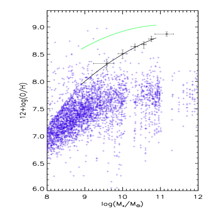
(a) $\alpha=0.01$

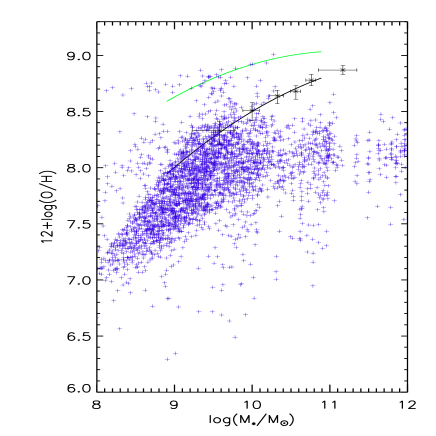
(b) $\alpha=0.05$

Figure 1: Response of the predicted mass-metallicity relation to a change in the star formation efficiency for galaxies at redshift $2.27$. The blue crosses represent an individual galaxy with stellar mass and metallicity predicted by the model and the black asterisks show the data from Erb et al. (2006). The green (upper) line shows the AMAZE best-fitting line for $z=0.07$ and the black (lower) line is the same curve fitted to the data at $z=2.27$.

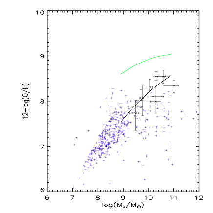
(a) $\alpha=0.01$

(b) $\alpha=0.05$

Figure 2: Response of the predicted mass-metallicity relation to a change in the star formation efficiency for galaxies at redshift $3.54$. The blue crosses represent an individual galaxy with stellar mass and metallicity predicted by the model and the black asterisks show the data from Maiolino et al. (2008). The green (upper) line shows the AMAZE best-fitting line for $z=0.07$ and the black (lower) line is the same curve fitted to the data at $z=3.54$.

4.1.2 Redshift Dependence of the SFR

With $\alpha$, $\epsilon$ and $\zeta$ held constant at their fiducial values $\beta$ was varied over the range $0<\beta<1.25$. The GalICS predictions for galaxies are shown in Fig. 3 ($z\approx 2.27$) and Fig. 4 ($z\approx 3.54$). Inspection of the plots show that $\beta$ has a distinguishable effect on the distribution of the mass and metallicities of the galaxies. At any given redshift increasing $\beta$ preserves (approximately) the number of galaxies predicted but the distribution favours more galaxies with a higher stellar mass and metallicity whilst preserving the trend which is a similar shape to the AMAZE calibration curve (equation 5). This follows from the fact that at constant redshift increasing $\beta$ results in the term $\left(1+z\right)^{\beta}$ in equation 3 being larger and thus it acts in a similar manner to $\alpha$. The same number of mergers are predicted so that the mass distribution is similar but not identical since the SFR does play a role in determining the mass of individual galaxies (Weidner et al., 2007).

As in the previous section a simple $\chi^{2}$ analysis would return lower results for increasing $\beta$, whereas we believe that the values for $\beta$ should not be higher than 1.

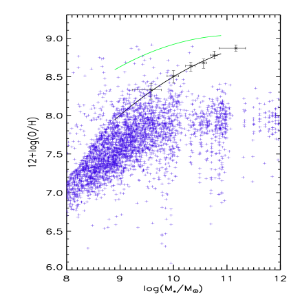
(a) $\beta=0$

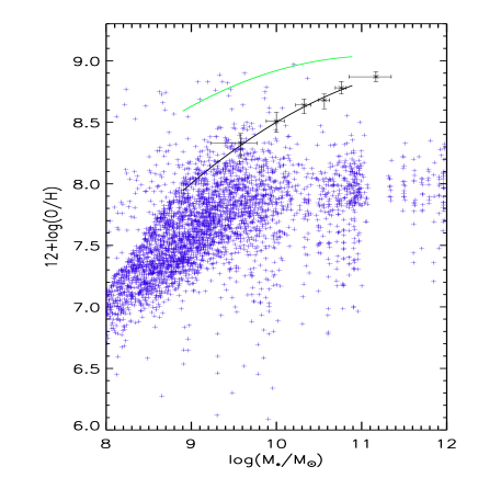
(b) $\beta=1.25$

Figure 3: Response of the predicted mass-metallicity relation to a change in the redshift dependence of the star formation rate for galaxies at redshift $2.27$. The blue crosses represent an individual galaxy with stellar mass and metallicity predicted by the model and the black asterisks show the data from Erb et al. (2006). The green (upper) line shows the AMAZE best-fitting line for $z=0.07$ and the black (lower) line is the same curve fitted to the data at $z=2.27$.

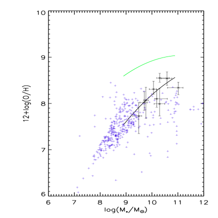
(a) $\beta=0$

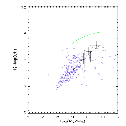
(b) $\beta=1.25$

Figure 4: Response of the predicted mass-metallicity relation to a change in the redshift dependence of the star formation rate for galaxies at redshift $3.54$. The blue crosses represent an individual galaxy with stellar mass and metallicity predicted by the model and the black asterisks show the data from Maiolino et al. (2008). The green (upper) line shows the AMAZE best-fitting line for $z=0.07$ and the black (lower) line is the same curve fitted to the data at $z=3.54$.

4.1.3 Supernova Feedback Efficiency

With $\alpha$ and $\beta$ held constant at their fiducial values $\varepsilon$ was varied over the range $0.1\leq\varepsilon\leq 1.0$. Following the discussion in section 2.3, this range is investigated in order to test the model however we do not use excessively large values in order to artificially fit relations hereafter. The plots in Figs. 5(a) and 5(b) show the mean mass and metallicity predicted in each of the six mass bins used by Erb et al. (2006) at $z=2.27$ and $z=3.54$ respectively. Fig. 5(a) shows that the effect of increasing epsilon at $z=2.27$ is to lower the average metallicity in each bin whilst preserving the overall shape of the relation. At higher values of $\varepsilon$, more gas is ejected from the galaxy thereby reducing the average metallicity in each bin. Thus the effect of changing $\varepsilon$ is to alter the offset of the relation without altering the slope. This effect is comparable to the one predicted by Finlator & Davé (2008) with the difference that we have a self consistent chemical evolution that includes the finite lifetimes of both SNIa and SNII. At $z=3.54$, Fig. 5(b) shows that changing the value of $\varepsilon$ has very little effect on the relation, especially in the low mass regime, and basically preserves the shape of the relation.

Mannucci et al. (2009), whose sample of LBGs at $z\sim 3$ (discussed in the introduction), have found that the effective yield (the amount of metals synthesised and retained within the ISM per unit stellar mass) decreases with increasing stellar mass for galaxies in their sample suggesting that galactic outflows cannot account for the shape of the mass-metallicity relation since their power is diminished in more massive galaxies and thus they cannot be responsible for the decreasing effective yields. Using chemical evolution models for galaxies of varying morphological types Calura et al. (2009) have found that the relation arises naturally, regardless of the morphology, if the SSFR is larger in more massive galaxies and that galactic outflows are not needed to explain the relation. As noted in the introduction, none of the models that focus solely on different outflow processes only have been able to fit the observed relation at $z=3.54$ and, taken together, these plots imply that outflows are only important in determining the low redshift relation whereas at higher redshifts, another mechanism is responsible for generating this relation, which may explain this lack of predictive power at higher redshifts. Considering these recent results, the findings of this section imply that it is the SFR-mass relation that generates the observed mass-metallicity relation and determines the slope at high redshift with outflows being important only for the low redshift properties.

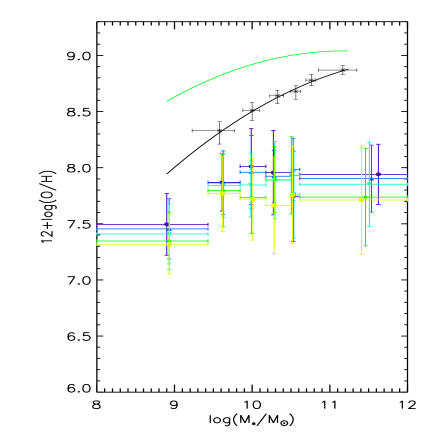
(a) $z=2.27$

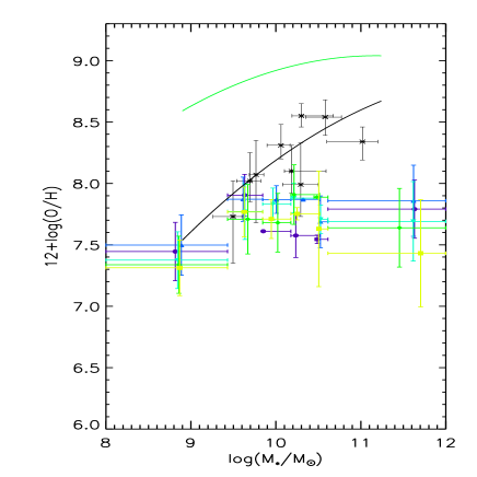
(b) $z=3.54$

Figure 5: The change in the average mass-metallicity relation when $\varepsilon$ is varied at redshift $2.27$ and $3.54$. The purple circles, dark blue upward-facing triangles, light blue downward-facing triangles, green diamonds and yellow squares show the average mass and metallicity in each of the six mass bins used by Erb et al. (2006) when $\varepsilon=0.1\,,0.3\,,0.5\,,0.8$ and $1.0$ respectively. The horizontal bars show the range of the mass bins and the vertical bars show one standard deviation in the metallicity. The black asterisks and line show the data from Erb et al. (2006) (Fig. 5(a)) or Maiolino et al. (2008) (Fig. 5(b)) and the black (lower) line shows the AMAZE best-fitting line for the observed relations at the respective redshifts. The green (upper) line shows the AMAZE best-fitting line for the observed relation at $z=0.07$.

4.2 Variation of the IMF

Using the free parameters held at their fiducial values the IMF was changed to the Kennicutt IMF (equation 2). Fig. 6 shows the predicted relation for galaxies at redshifts $2.27$ and $3.54$. Comparing Fig. 6 to Figs. 1-4 it is clear that both IMFs predict similar shaped relations at both redshifts. As a matter of fact, the Kennicutt IMF predicts lower values than both Salpeter and observation at $z=2.27$. At $z=3.54$ both IMFs predict similar distributions that are both in the same region as observed. Only the Salpeter IMF produces a distribution that has many galaxies with similar masses and metallicities to observations at both redshifts, which indicated that it may have been able to reproduce the observed relation given the right values of the free parameters. For this reason only the Salpeter IMF was investigated quantitatively to see if it could reproduce the observed relation at both redshifts.

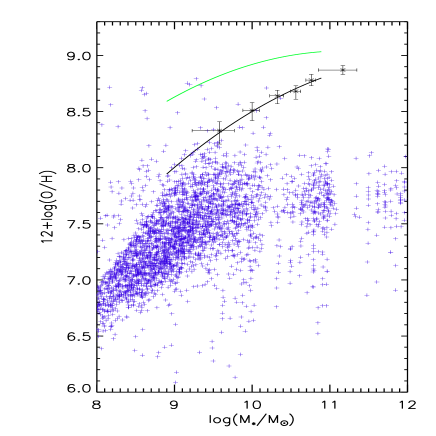
(a) $z=2.27$

(b) $z=3.54$

Figure 6: Predicted mass-metallicity relation using the Kennicutt IMF with the free parameters held at their fiducial values. The blue crosses represent an individual galaxy with stellar mass and metallicity predicted by the model and the green (upper) line shows the AMAZE best-fitting line for $z=0.07$. The black asterisks show the data from Erb et al. (2006) (6(a)) or the data from Maiolino et al. (2008) (6(b)) and the black (lower) line shows the AMAZE best-fitting line for $z=2.27$ (6(a)) or $z=3.54$ (6(b)).

5 Discussion

Examination of the plots in Figs. 1 to 4 reveals that, no matter the value of any parameter, there is a definite trend in the predicted distribution of stellar mass and metallicity. This is the known trend of increasing metallicity with stellar mass that follows a shape similar to the AMAZE calibration curve (equation 5) at both redshifts. The plots also show a scatter that is comparable to the scatter seen in the data from Tremonti et al. (2004) at $z\approx 0$ independent of the value of any of the free parameters. Finally most of the galaxies have metallicities that lie below the data from Tremonti et al. (2004) ($z\approx 0$) and the AMAZE best-fitting curve for $z=0.07$ indicating that most of the galaxies had a lower metallicity in the past than today. This is consistent with stellar and galactic chemical evolution theory (Pagel, 1998) and is an indication that the model simulates the physics correctly.

The results of section 4.1 showed that the model could reproduce the observed mass-metallicity relation and suggested that a good fit to the current observations could be achieved by a suitable choice of parameters and IMF. Section 4.1.3 revealed that the effects of varying $\varepsilon$ were much smaller than varying $\alpha$ and $\beta$ hence only these two parameters were varied. Predictions were generated using parameters in the range $0.01\leq\alpha\leq 0.05$ and $0\leq\beta\leq 1.25$ with $\varepsilon$ and $\zeta$ held constant at their fiducial values.

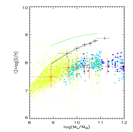
(a) $z=2.27$

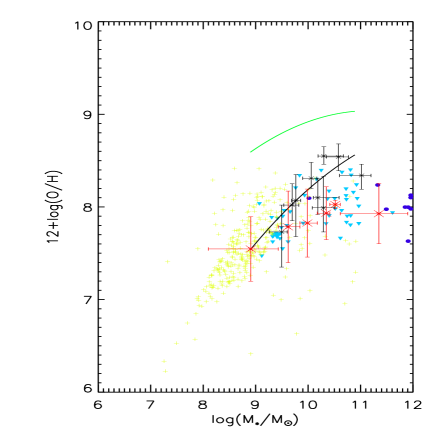
(b) $z=3.54$

Figure 8: Predicted mass-metallicity relation using the best-fitting parameters $\alpha=0.02$, $\beta=1.0$, $\varepsilon=0.15$ and $\zeta=0.3$ and the Salpeter IMF (equation 2). The yellow crosses represent galaxies with $\textrm{SFR}<10M_{\odot}\textrm{yr}^{-1}$, the light blue triangles represent galaxies with $10\leq\textrm{SFR}<30M_{\odot}\textrm{yr}^{-1}$ and the dark blue circles represent galaxies with $\textrm{SFR}\geq 30M_{\odot}\textrm{yr}^{-1}$. The green (upper) line shows the AMAZE best-fitting line for $z=0.07$ and the black asterisks show the data from Erb et al. (2006) (8(a)) or Maiolino et al. (2008) (8(b)). The black (lower) line shows the AMAZE best-fitting line for $z=2.27$ (8(a)) or $z=3.54$ (8(b)). The red crosses show the average mass and metallicity in each of the 6 mass bins used by Erb et al. (2006), the horizontal bars show the mass bins and the vertical bars show one standard deviation in the metallicity.

It was found that the parameters that best match the observed relations were $\alpha=0.02$ and $\beta=1.0$. The plots in Fig. 8 show the predicted relations at both redshifts using the best-fitting parameters found in section 5. Fig. 8(a) shows that the observed relation is not predicted at $z=2.27$, instead the predicted distribution has a large scatter and shows a similar shaped trend to but lies mainly below the observations of Erb et al. (2006). Fig. 8(b) shows that the observed relation (Maiolino et al., 2008) is predicted at $z=3.54$ with a comparable scatter. At both redshifts the majority of predicted galaxies lie below the observations of Tremonti et al. (2004) and the AMAZE $z=0.07$ best-fitting relation (equation 5). At both redshifts we predict a flatter relation than observed. This effect is particularly clear at $z=2.27$ where none of the predicted massive galaxies are consistent with the observed ones even taking into account the errors on the latter. The situation is less extreme in the high redshift case, nevertheless it may be a symptom of some missing physics in the model. We will thoroughly discuss such problems in the rest of this section. To gain better insights on the model galaxies it is worth, however, first having a look at the predicted SFRs, since the predicted flattening in the mass-metallicity relation may come from issues with the manner in which GalICS predicts them. Both plots show the predicted galaxies stratified by SFR into the three bins $\textrm{SFR}<10M_{\odot}\textrm{yr}^{-1}$, $10\leq\textrm{SFR}<30M_{\odot}\textrm{yr}^{-1}$ and $\textrm{SFR}\geq 30M_{\odot}\textrm{yr}^{-1}$. To some extent, the predicted SFRs should only be compared with each other and any direct comparison with experimentally observed values should be treated equivocally. In fact, GalICS predictions are average values over the entire galaxy and over the timestep, whereas observations look at more central regions (see below) and yield an instantaneous SFR value. We can thus gain more insight from the comparison of the relative differences and evolution in the predicted and observed SFRs than their numerical values. Indeed, our predicted SFRs (see Fig. 7 below) are quite lower than those observed by Maiolino et al. (2008) who find an average SFR of $\sim$100$M_{\odot}$yr^-1 but are consistent with those from Erb et al. (2006) who find a median value of $\sim 30M_{\odot}$yr^-1, although we do not reproduce some of their extreme cases (with SFRs $\sim 300M_{\odot}$yr^-1).

While a (small) fraction of the disagreement can be explained by a small difference in the adopted upper mass limit for the IMF between our model and the value adopted by the observational works, we believe that this is a general problem of semi-analytic models (see, for example, Khochfar & Silk, 2009, and references therein). For instance, if the gas accretion and cooling are uneven over a timestep, the SFR may present spikes that are in better agreement with the values reported by both Maiolino et al. (2008) and Erb et al. (2006). The dynamics of these high redshift galaxies are not always consistent with a smooth star forming disc, instead they are highly turbulent (see, for example, Genzel et al., 2008) and a large fraction do not seem to rotate (for example, those observed by Law et al., 2009). A similar discussion of the dynamics of the AMAZE galaxies is given in Gnerucci et al. (2010). This star forming mode is not yet accounted for in GalICS and, perhaps, the high value for $\beta$ that we obtain should be interpreted as a warning: the treatment of the star formation must be improved, possibly taking into account gas supplies that are enhanced by cold streams. Namely the required boosting in the SFR is not only given by an increase in the efficiency, but also by augmenting the gas supply. This has to preferentially happen in more massive galaxies, where the disagreement with observations occur and, as can be inferred from the results presented in the previous sections, a much better fit could be obtained by differentially increasing $\alpha$ and $\beta$ at the high mass end with respect to their fiducial values, namely those that correctly fit the low mass end. On the other hand Mannucci et al. (2009) have observed the SFR as a function of $\log\left(M_{*}/M_{\odot}\right)$ for another sample of galaxies at $z\sim 3$ and have found, on average, a lower SFR than in the AMAZE sample, while at the same time the O abundances are similar to those we are using in this work. In particular, in the mass range $9.5\leq\log\left(M_{*}/M_{\odot}\right)\leq 10.5$ the average SFR that we predict is $\langle\textrm{SFR}\rangle=30.0M_{\odot}$yr^-1 at $z=2.27$. We note that this value has been corrected to account for the difference in IMFs. The range of the deviation from this average is (approximately) $75M_{\odot}$yr^-1 at the three standard deviation level. At $z=3.54$ and for similar masses we find $\langle\textrm{SFR}\rangle=9.4\pm 26.4M_{\odot}$yr^-1 at the three standard deviation level.

We note that there are many more predicted galaxies in our bin than Mannucci et al. (2009) and that the standard deviation in our SFR is due to this large number of predicted galaxies whereas theirs is due to experimental uncertainties involved with their observation. Therefore, another possibility, is that, while AMAZE probes the systems with the highest SFR, the model adopted here gives values that are more “typical” for high redshift galaxies. Nevertheless, a successful model should predict also the extreme galaxies, unless those with extreme SFRs cannot be captured by either the spatial resolution or the lack of physics. Finally, we note that the observed SFRs discussed above have been derived by assuming exponentially declining SF histories. Maraston et al. (2010) have shown that this assumption might lead to an overestimate of the SFR with respect to other, more realistic SF histories, especially when the age is not constrained to be larger then the e-folding time of the assumed exponentially declining SFR. Similarly, Maiolino et al. (2008) have noted that the fits that yield the SFR in the AMAZE sample sometimes return unrealistically small ages (below 50 Myr) if not suitably constrained.

In Fig. 7 we plot the predicted SFR against stellar mass. It is evident from this Fig. (as well as Fig. 8 discussed below) that galaxies with larger stellar mass and metallicities have higher SFRs and thus our predicted relation is one between SFR and mass, consistent with the recent predictions of Calura et al. (2009) as well as the observational findings of Mannucci et al. (2009). It is also clear from the plots that we do find that, at any given mass, more pristine galaxies have a large SFR and viceversa, in agreement with the recent suggestion by Mannucci et al. (2010) that the mass-metallicity relation is, in fact, a mass-SFR-metallicity surface. However, if we use the new “variable” suggested by Mannucci et al. (2010), namely $\log\left(M_{*}\right)-0.32\log\left(\textrm{SFR}\right)$ instead of $\log(M_{*})$, as the abscissa then we do not find a significant decrease in the scatter. Here we do not make any inferences or draw any conclusions about the relationship that Mannucci et al. (2010) have proposed but leave a more comprehensive comparison for future work where we intend to use a forthcoming, updated and refined version of GalICS that is better calibrated on the $z=2.27$ and $z=3.54$ mass-metallicity relation.

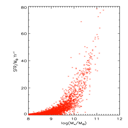
(a) $z=2.27$

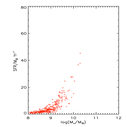
(b) $z=3.54$

Figure 7: The predicted SFR as a function of stellar mass for galaxies at redshift $z=2.27$ and $z=3.54$. The red asterisks show individual predicted galaxies with a given stellar mass and SFR.

Our inability to fit the relation at $z=2.27$ may be due to differences between the regions of the galaxies sampled by observation and by GalICS. For instance, the observations of Erb et al. (2006) are obtained using a long slit spectrometer with an aperture of $0.75^{\prime\prime}$, corresponding to a radius (half-aperture) on the galaxy of only $3.6$ kpc at $z=2.27$ (Maiolino et al., 2008). This implies that Erb et al. (2006) only sample the central region of the most massive - hence larger - galaxies, whereas less massive systems are probed out to larger radii. Local galaxies have metallicity gradients that, combined with the fixed aperture, bias the mass-metallicity relation. As shown by Cresci et al. (2010, in press) high-redshift star forming systems have a complex metallicity structure, however further study is needed to assess its impact on the observed relation. On the theoretical side, GalICS calculates the average metallicity over the entire galaxy (Pipino et al., 2009), including the outer regions which are metal poor. We will come back on this aspect of this problem later when discussing the role of the bulge and the burst components. AMAZE (Maiolino et al., 2008) use integral field spectroscopy to measure their metallicities, extracting the spectral information using a $0.7^{\prime\prime}$ aperture which corresponds to a similar radius to the Erb et al. (2006) sample. Moreover, the observed size evolution (see, for example, Law et al., 2007) of LBGs between $z\sim 3.5$ and $z\sim 2$, is rather mild, therefore we deem it unlikely that Erb et al. (2006) sample a much smaller portion of these galaxies - at a given fixed mass - than AMAZE, in order to justify an even larger departure of the models from the observations at $z=2.27$ than at $z=3.54$. Whilst these effects may be present (indeed we cannot rule them out) and can partly explain the difference between our models’ predictions and observations, we believe that the disagreement at the high mass end has more to do with the treatment of the physics and the assumptions in the model.

To better explain the lack of chemical evolution in the most massive galaxies we have performed several tests using a chemical evolution model (Pipino & Matteucci, 2004) with the same setup (in terms of both IMF and stellar yields) and allowing for different infall and star formation timescales. These models, that follow the evolution of a single galaxy, have the advantage of giving a self-consistent description of the chemical evolution, whilst using a simpler parametrisation for the accretion and the star formation histories than we use in GalICS. In passing, we note that these models are, in essence, the same ones that are used by Calura et al. (2009) to study the AMAZE galaxies in the context of their monolithic collapse. As far as the adopted star formation rate is concerned, it is given by the same formula as GalICS (equation 3), with the absence of any redshift dependence i.e. $\beta=0$. The star formation timescale $t_{\textrm{SF}}=t_{\textrm{dyn}}/\alpha$ and we assume an exponentially decreasing gas infall law (i.e. $\propto e^{-t/\tau}$, where $\tau$ is the infall timescale), that is not linked to any Dark Matter accretion history. By running these chemical evolution models for a large range of different combinations of $\tau$ and $t_{\textrm{SF}}$, we confirm that a relatively high O abundance ($12+\log\left(O/H\right)>7.5$) is attained within a few 100 Myr. At the same the time stellar mass is quickly built up. This is why GalICS, whose predicted galaxies feature a differing SFR and different accretion/merging histories, predicts a steep mass-metallicity relation at low masses/younger (relatively) ages. What differs is the subsequent evolution. For a star formation timescale much shorter than the infall timescale, the chemical evolution model show a metallicity $12+\log\left(O/H\right)>8.5$ already at 200 Myr and a very mild evolution after that. On the other hand, when the star formation timescale is comparable to the infall timescale and both are of the order of 1 Gyr, galaxies attain a metallicity $12+\log\left(O/H\right)\approx 8$ in the same timescale and a further 0.5 dex increase in the O abundance would take more than 1 Gyr (i.e. the time elapsed between z=3 and z=2). In other words, since this latter case is typical in GalICS, it is easy for the model galaxies to quickly attain $12+\log\left(O/H\right)\approx 7.5-8$ at redshift 3, hence reproducing the average observed value, but then the predicted metal enrichment in the redshift range 3-2 is slower than that inferred from the observations because the star formation is not efficient enough. The former case (star formation timescale shorter than infall timescale), instead, characterises the monolithic collapse models used by Calura et al. (2009) to reproduce the AMAZE data. It must also be remembered that the $\beta$-boosting at z=3 is by a factor of 4, whereas the boosting at z=2 is by a factor of 3. Hence, the redshift dependence of the SFR in such a “narrow” range is quite mild and will not necessarily drive major changes in the predicted mass and metallicities (see Section 4) in this time interval.

Moreover, at higher masses, a fair fraction (approximately 20%) of model galaxies have had at least one merger. Therefore some older galaxies could have become quiescent, or at least have a sizable number of stars in the bulge component. In this latter case, even if the O abundances are quite high ($12+\log\left(O/H\right)>8.5$) in the gas associated with the bulge component, the SFR and the gas mass in this component are much lower than in the disc. Were such a strict separation between disc and bulge in the models present also in actual galaxies, the bulge metallicity would not be easily observed. This seems to be at variance with actual observations (see, for example, Law et al., 2007) that do not detect a drop in the rest-frame UV flux in the central regions of the galaxies. This fact may hint that the disc/burst/bulge decomposition of model galaxies that well characterises local galaxies is not a good approximation of the complex structure of high redshift star forming systems. Modifications such that, for instance, the metal rich gas from the bulge component could enrich the discs, may help in reconciling such models with observations.

At the same time, as it can clearly be perceived from the fact that there are many more galaxies in the z=2 figures as opposed to the z=3 ones, we predict a large number of new galaxies that appear during the elapsed time interval. The youngest ones have stellar masses below $10^{10}M_{\odot}$ and low metallicities, thus biasing the predicted mass-metallicity relation to lower values and affecting the predicted evolution. Therefore, in order to improve the agreement with observations, one can apply a SFR/age cut to the predicted sample of galaxies. Given the difficulties in predicting the correct SFRs - see above - this has not been attempted.

A closer inspection of our galaxies show that the metallicity increases with decreasing gas mass fraction almost as expected in a simple closed box model of chemical evolution, namely $Z\propto ln(M_{tot}/M_{gas})$. The gas fraction is almost constant (around 0.8) with total baryonic mass (at a fixed redshift) in the high mass regime, whereas it exhibits a large scatter at the low-mass end. On the other hand it strongly decreases with stellar mass, although with increasing scatter. This is because the SFR is constant for galaxies with stellar mass below $10^{10}M_{\odot}$, becoming proportional to the stellar mass above this limit (c.f. Fig. 9 in Mannucci et al. (2009)). Only for the most massive galaxies (in terms of their stellar mass), does the gas fraction rise again to (approximately) $0.8$. This is basically what we see in the mass-metallicity plots: the metallicity increases with stellar mass up to $\sim 10^{10}M_{\odot}$ where it then flattens out in the most massive galaxies (where the gas fraction is higher again). As explained above, in these systems the star formation is not efficient enough compared to the inflow of primordial gas. Indeed, as shown by Calura et al. (2009), the high mass end of the z=3 mass-metallicity relation cannot be reproduced by the “local” disc, but proto-spheroids with very high SFR, such that their O abundance quickly jumps to solar values in a few Myr, are needed. At variance with such a model, where the galaxy morphology is assumed, GalICS galaxies may have three components (disc, bulge and burst, see Section 2 and Hatton et al. (2003), for more details) that co-exist at the same time and whose presence is linked to the evolutionary path of the galaxies. Here we remind the reader that we show the abundances predicted for the disc component of each galaxy only in order to have a fair comparison with the observations that sample quite a large region compared to the assumed sizes of both the bulge and burst components in the model (whenever they are present). The results do not change if we show the abundances averaged over the three components because the mass in the cold phase of the disc is much larger than that in the bulge (where we predict gas mass fraction well below 0.1) or in the burst. In these latter components we predict $12+\log\left(O/H\right)>8.5$ in the majority of the galaxies, however, such a high O abundance is diluted in the mass averaging. We have already noted that observations sample the inner regions of the galaxies. On the other hand, we present the results pertaining to the entire disc because the nominal spatial resolution of GalICS is $\sim$30 kpc. If we had enough spatial resolution to make predictions about the inner $\sim$4 kpc only, it is likely that: i) the local density would make the local SFR higher, hence the metal enrichment quicker and ii) the dilution of the metals in the bulge and in the burst by means of the inner disc gas would be lower (meaning a higher metallicity in that region of the disc, lower fractional contribution in the mass averaging). Finally, we note that on the abscissa of all the Figs. discussed so far, we plot the total stellar mass, summed over the three component. Since bulges and bursts tend to be more frequent at the high mass end, where galaxies are older and had more time to evolve and merge, this implies that we stretch the mass axis without an increase in the O abundance, hence obtaining an artificially flatter (by a small amount) and more extended to high masses mass-metallicity relation than the one expected for a pure disc.

One possible way out would involve making predictions that take into account the three component, without computing an average O abundance. For instance, one could use the discs to explain the low mass end of the mass metallicity relation, whereas bursts and bulges could explain the high mass end (see also Calura et al., 2009). As noted above, the bulges cannot be directly compared with the observations because it is assumed that the SFR in this component can involve only gas returned from stars, hence the predicted SFR are lower than those in the disc. Using the bulges instead of the discs at the high mass end, where they are more abundant, will lead to an increase in the slope of the predicted mass-metallicity relation, at the expense of an even poorer agreement between the observed and predicted SFR.

At z=2, nearly 15% of the galaxies feature a burst component. In such a component, the galaxies exhibit SFRs comparable to, or even a factor of $\sim$2 higher than, the disc and the predicted O abundances are $8<12+\log\left(O/H\right)<9$, so one may be tempted to use only the predicted properties of the burst only to compare with observations. The problems with this last scenario are numerous. In the first place, the burst component is assumed to have a radius that is typically below 1 kpc, hence smaller than both that of the disc and the aperture used by observers. We find it difficult to explain the properties of observed galaxies only by means of such a centrally concentrated component. Moreover, one has to devise a reason to bias the observations in favour of a “burst” only above a given mass ($\sim 10^{10}M_{\odot}$) in order to steepen the mass-metallicity relation at the high mass end. In part, such a bias can be granted by the fact that observed samples are selected according to their SFR. However, since the model switches the burst component on as a consequence of mergers, the hypothetical solution of having a greater frequency of burst components in the more massive galaxies is at variance with the fact that a fraction of the observed galaxies do not show such signatures. Moreover, recent observations (for example those of Förster Schreiber et al., 2009) indicate that galaxies that are observed with a regularly rotating disc are preferentially higher mass systems. However, these discs still have large amounts of random motions and turbulence can be fairly thick. Future developments of the models should implement the possibility that “bursts” are not only centrally located. Instead SF clumps would be distributed in the disc, as also discussed above when comparing predicted and observed SFRs.

The net effect of the changes suggested above should create a typical galaxy formation path in which, broadly speaking, $\alpha$ increases with galactic mass. Indeed a direct increase of $\alpha$ with mass may be achieved by directly incorporating the suggestion by (Pipino et al., 2009) on the positive feedback by the central black hole. Such a change can be easily implemented in monolithic formation models, however it is more difficult to devise a mechanism in a scenario where larger galaxies are formed through mergers of smaller companion. This is where the study of the mass-metallicity relation at $z\approx 3$ provides leverage: many (predicted) galaxies have not undergone any mergers yet and sot he effect of these mergers is kept at a minimum level. These mergers tend to produce high mass galaxies with lower metallicities than those that have evolved in the standard manner and thus (in general) flatten the relation. Hence the observed mass-metallicity relation is, in fact, giving us insight into the SFR-mass and inflow-mass relations. To be more quantitative, from the investigation done in Section 4 we can infer that if the value of $\alpha$ is kept at the fiducial GalICS value at the low mass end, whereas its value is increased by a factor of at least 3 at the high mass end, the predicted mass-metallicity relation would be considerably steeper and in better agreement with observations. The reader should note that this is an illustrative example to provide insight into the manner in which current models should be modified in order to improve them in this respect and that unnaturally fixing $\alpha$ as a function of stellar mass is only an artificial solution and is not the correct method by which this can be achieved. In passing, we note that these solutions may also alleviate the problems that semi-analytic models have in reproducing the abundance ratio-mass relations in present-day elliptical galaxies (Pipino et al., 2009).

We also note that, although variation of the parameters significantly changes the prediction of the mass-metallicity relation at high redshift, the effect at low redshift is much less evident.

On the other hand, examination of the predicted distribution at $z=0$ shows that the evolution in metallicity between $z=3.54$ and $z=0.07$ agrees with the observed evolution (Tremonti et al., 2004; Maiolino et al., 2008). This is shown in Fig. 9. Previous models (for example De Lucia et al. (2004), Kobayashi et al. (2007) and others discussed in the introduction) often fit the relation at one redshift only and the redshift evolution is not tested to $z=0$ (see Maiolino et al. (2008) section 7.5 for a discussion). We have fitted the observed relations at both $z=3.54$ and $z\approx 0$ and hence the model is more tightly constrained. We have not been entirely successful in fitting the observed relation at all redshifts however we have attempted to constrain it in different regimes and predict the observed evolution of the relation from $z=3.54$ to $z=0$. Furthermore, we have found that outflows are not the origin of the relation and only effect its low redshift evolution and hence we have not needed to impose different outflow models to fit at specific redshifts. Nor have we needed to fine-tune the efficiency of supernova feedback.

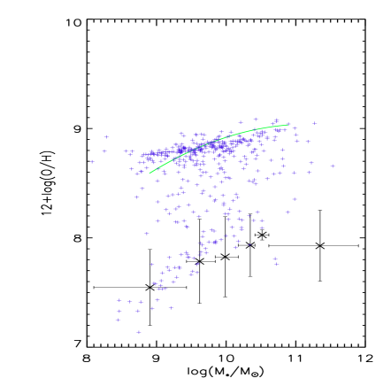
Figure 9: The predicted evolution from $z=3.54$ to $z\approx 0$. The black crosses show the average mass and metallicity in each of the six mass bins used by Maiolino et al. (2008) at $z=3.54$ using the best-fitting parameters. The horizontal bars show the range of each mass bin and the vertical bars show one standard deviation in the metallicity. The AMAZE best-fitting curve (equation 5) at $z=0.07$ is shown by the green line and the blue crosses show the predicted mass-metallicity relation at $z\approx 0$.

6 Conclusions

The relation between stellar mass and gas-phase metallicity has been well documented over the range $0\leq z\leq 3.54$ (Tremonti et al., 2004; Erb et al., 2006; Maiolino et al., 2008). Despite this many hydrodynamical and semi-analytic $N$-body simulations of galaxy formation have been unable to predict the correct relation over a suitable redshift range (De Lucia et al., 2004; De Rossi et al., 2007; Mouchine et al., 2008). In this paper we have fitted the observed relation at $z\approx 3.54$ using an updated version of GalICS given in Pipino et al. (2009) and have reproduced the observed relation at $z\approx 0$. The model uses a $\Lambda$CDM cosmology taken from WMAP3 (Spergel et al., 2007) and includes outflows due to type-II supernovae since previous work (De Rossi et al., 2007) has shown that these are needed to reproduce the observed relation. Many free parameters are included that control the star formation efficiency, redshift dependence of the SFR, type-II supernova feedback efficiency and the halo recycling efficiency which were varied separately in order to achieve the best possible fit to observation (Maiolino et al., 2008). Here we summarise the results of the simulations.

Firstly, we have found that the effect of varying the supernova feedback efficiency has little impact on the relation at high redshift but does have a small effect at lower values. We have also predicted that more massive galaxies have higher SFRs than less massive ones. These two results taken together support recent findings (Mannucci et al., 2009; Calura et al., 2009) that it is the SFR-mass relation in galaxies and not galactic outflows that is responsible for the origin and evolution of the relation although the cumulative effects of outflows do affect the low redshift evolution. Secondly, a better agreement between the predicted and the observed average metallicity at a given redshift can be obtained by assuming that the SFR that has a strong redshift dependence, proportional to $1+z$, which is slightly stronger than other models have used in the past (Cattaneo et al. (2006) uses $\left(1+z\right)^{0.6}$). At the same time, the predicted SFRs are lower than the observed values at $z\sim 3$, but are consistent at lower redshifts. These facts may point to the need for a revision of the SFR recipes in a future generation of semi-analytical models. Thirdly, the observed relation at $z=3.54$ is reproduced well with a scatter in the distribution of stellar mass and metallicity comparable to observations (Maiolino et al., 2008). However, the predicted relation is flatter at the high mass end. Also, we fail to reproduce the relation at $z=2.27$ (Erb et al., 2006), where the flattening in the high mass regime becomes more evident. We discuss several reasons for this disagreement, stemming from both theoretical and observational biases. We argue that if observations are preferentially selecting galaxies with high SFRs and the measured abundances mirror those in these “bursts” rather than averages over the three components, we might solve the problem of the flattening by using the abundances predicted in the “burst” rather than in the disc component of the model galaxies. This is a rather ad hoc solution and presumably means that future models should take into account that, at high redshifts, either the SF occurs in clumps rather than in a smooth disc or the star formation efficiency is boosted preferentially in the most massive galaxies by, for example, positive AGN feedback Pipino et al. (2009). We note, that the model does reproduce the observed evolution to $z=0$. The efficiency of outflows was found to have only a minimal effect on the predicted distribution. Finally, we have seen that low-mass galaxies are best fitted to the relation using a low star formation efficiency whereas the converse is true regarding high-mass galaxies. This observation supports the findings of Maiolino et al. (2008) and thus galaxy downsizing may be the origin of the ubiquitously observed relation.

References

- Bower et al. (2010) Bower R. G., Vernon I., Goldstein M., Benson A. J., Lacey C. G., Baugh C. M., Cole S., Frenk C. S., . 2010, ArXiv e-prints
- Brodie & Huchra (1991) Brodie J. P., Huchra J. P., 1991, ApJ, 379, 157
- Calura et al. (2009) Calura F., Pipino A., Chiappini C., Matteucci F., Maiolino R., 2009, A&A, 504, 373
- Cattaneo et al. (2006) Cattaneo A., Dekel A., Devriendt J., Guiderdoni B., Blaizot J., 2006, MNRAS, 370, 1651
- Cescutti & Chiappini (2010) Cescutti G., Chiappini C., 2010, A&A, 515, A102+
- Conroy et al. (2008) Conroy C., Shapley A. E., Tinker J. L., Santos M. R., Lemson G., 2008, ApJ, 679, 1192
- De Lucia et al. (2004) De Lucia G., Kauffmann G., White S. D. M., 2004, MNRAS, 349, 1101
- De Rossi et al. (2007) De Rossi M. E., Tissera P. B., Scannapieco C., 2007, MNRAS, 374, 323
- Erb et al. (2006) Erb D. K., Shapley A. E., Pettini M., Steidel C. C., Reddy N. A., Adelberger K. L., 2006, ApJ, 644, 813
- Erb et al. (2006) Erb D. K., Steidel C. C., Shapley A. E., Pettini M., Reddy N. A., Adelberger K. L., 2006, ApJ, 647, 128
- Faber (1973) Faber S. M., 1973, ApJ, 179, 731
- Ferreras & Silk (2003) Ferreras I., Silk J., 2003, MNRAS, 344, 455
- Feulner et al. (2005) Feulner G., Gabasch A., Salvato M., Drory N., Hopp U., Bender R., 2005, ApJ, 633, L9
- Finlator & Davé (2008) Finlator K., Davé R., 2008, MNRAS, 385, 2181
- Förster Schreiber et al. (2009) Förster Schreiber N. M., Genzel R., Bouché N., Cresci G., Davies R., Buschkamp P., Shapiro K., Tacconi L. J., Hicks E. K. S., Genel S., Shapley A. E., Erb D. K., Steidel C. C., Lutz D., Eisenhauer F., Gillessen S., 2009, ApJ, 706, 1364
- Garnett & Shields (1987) Garnett D. R., Shields G. A., 1987, ApJ, 317
- Genzel et al. (2008) Genzel R., Burkert A., Bouché N., Cresci G., Förster Schreiber N. M., Shapley A., Shapiro K., Tacconi L. J., Buschkamp P., Cimatti A., Daddi E., Davies R., Eisenhauer F., Erb D. K., Genel S., Gerhard O., Hicks E., 2008, ApJ, 687, 59
- Gnerucci et al. (2010) Gnerucci A., Marconi A., Cresci G., Maiolino R., Mannucci F., Calura F., Cimatti A., Cocchia F., Grazian A., Matteucci F., Nagao T., Pozzetti L., Troncoso P., 2010, ArXiv e-prints
- Greggio (2005) Greggio L., 2005, A&A, 441, 1055
- Guiderdoni et al. (1998) Guiderdoni B., Hivon E., Bouchet F. R., Maffei B., 1998, MNRAS, 295, 877
- Hatton et al. (2003) Hatton S., Devriendt J. E. G., Ninin S., Bouchet F. R., Guiderdoni B., Vibert D., 2003, MNRAS, 343, 75
- Helmboldt et al. (2004) Helmboldt J. F., Walterbos R. A. M., Bothun G. D., O’Neil K., de Blok W. J. G., 2004, ApJ, 613, 914
- Iwamoto et al. (1999) Iwamoto K., Brachwitz F., Nomoto K., Kishimoto N., Umeda H., Hix W. R., Thielemann F., 1999, ApJ, 125, 439
- Juneau et al. (2005) Juneau S., Glazebrook K., Crampton D., et al., 2005, ApJ, 619, L135
- Kennicutt et al. (1994) Kennicutt Jr. R. C., Tamblyn P., Congdon C. E., 1994, ApJ, 435, 22
- Kewley & Ellison (2008) Kewley L. J., Ellison S. L., 2008, ApJ, 681, 1183
- Khochfar & Silk (2009) Khochfar S., Silk J., 2009, ApJ, 700, L21
- Kobayashi et al. (2007) Kobayashi C., Springel V., White S. D. M., 2007, MNRAS, 376, 1465
- Köppen et al. (2007) Köppen J., Weidner C., Kroupa P., 2007, MNRAS, 375, 673
- Law et al. (2009) Law D. R., Steidel C. C., Erb D. K., Larkin J. E., Pettini M., Shapley A. E., Wright S. A., 2009, ApJ, 697, 2057
- Law et al. (2007) Law D. R., Steidel C. C., Erb D. K., Pettini M., Reddy N. A., Shapley A. E., Adelberger K. L., Simenc D. J., 2007, ApJ, 656, 1
- Lequeux et al. (1979) Lequeux J., Peimbert M., Rayo J. F., Serrano A., Torres-Peimbert S., 1979, A&A, 80
- Lilly et al. (1996) Lilly S. J., Le Fevre O., Hammer F., Crampton D., 1996, ApJ, 460, L1+
- Lu et al. (2010) Lu Y., Mo H. J., Weinberg M. D., Katz N. S., 2010, ArXiv e-prints
- Maiolino et al. (2008) Maiolino R., Nagao T., Grazian A., et al., 2008, A&A, 488, 463
- Mannucci et al. (2010) Mannucci F., Cresci G., Maiolino R., Marconi A., Gnerucci A., 2010, ArXiv e-prints
- Mannucci et al. (2009) Mannucci F., Cresci G., Maiolino R., Marconi A., Pastorini G., Pozzetti L., Gnerucci A., Risaliti G., Schneider R., Lehnert M., Salvati M., 2009, MNRAS, 398, 1915
- Maraston et al. (2010) Maraston C., Pforr J., Renzini A., Daddi E., Dickinson M., Cimatti A., Tonini C., 2010, ArXiv e-prints
- Matteucci & Recchi (2001) Matteucci F., Recchi S., 2001, ApJ, 558, 351
- Mouchine et al. (2008) Mouchine M., Gibson B. K., Renda A., Kawata D., 2008, ArXiv e-prints
- Nagao et al. (2006) Nagao T., Maiolino R., Marconi A., 2006, A&A, 459, 85
- Oppenheimer et al. (2009) Oppenheimer B. D., Davé R., Kereš D., Fardal M., Katz N., Kollmeier J. A., Weinberg D. H., 2009, ArXiv e-prints
- Pagel (1998) Pagel Bernard E. J., 1998, Nucleosynthesis and Chemical Evolution of Galaxies. CUP, Cambridge, UK
- Pérez-González et al. (2008) Pérez-González P. G., Rieke G. H., Villar V. o., 2008, ApJ, 675, 234
- Pipino et al. (2009) Pipino A., Devriendt J. E. G., Thomas D., Silk J., Kaviraj S., 2009, A&A, 505, 1075
- Pipino & Matteucci (2004) Pipino A., Matteucci F., 2004, MNRAS, 347, 968
- Pipino et al. (2009) Pipino A., Silk J., Matteucci F., 2009, MNRAS, 392, 475
- Recchi et al. (2004) Recchi S., Matteucci F., D’Ercole A., Tosi M., 2004, A&A, 426, 37
- Salpeter (1955) Salpeter E. E., 1955, ApJ, 121, 161
- Silk (2003) Silk J., 2003, MNRAS, 343, 249
- Skillman et al. (1989) Skillman E. D., Terlevich R., Melnick J., 1989, MNRAS, 240, 563
- Somerville & Primack (1999) Somerville R. S., Primack J. R., 1999, MNRAS, 310, 1087
- Spergel et al. (2007) Spergel D. N., Bean R., Doré O., et al., 2007, ApJ, 170, 377
- Spergel et al. (1997) Spergel D. N., Lilly S. J., Steidel C., 1997, Proceedings of the National Academy of Science, 94, 2783
- Springel (2005) Springel V., 2005, MNRAS, 364, 1105
- Strickland & Heckman (2009) Strickland D. K., Heckman T. M., 2009, ApJ, 697, 2030
- Thomas et al. (2007) Thomas D., Maraston C., Schawinski K., Sarzi M., Joo S., Kaviraj S., Yi S. K., 2007, in A. Vazdekis & R. F. Peletier ed., IAU Symposium Vol. 241 of IAU Symposium, Environment and the epochs of galaxy formation in the SDSS era. pp 546–550
- Tremonti et al. (2004) Tremonti C. A., Heckman T. M., Kauffmann G., et al., 2004, ApJ, 613, 898
- Weidner et al. (2007) Weidner C., Köppen J., Kroupa P., 2007 Vol. 241 of IAU Symposium. pp 120–121