Preparing thermal states of quantum systems by dimension reduction

Abstract

We present an algorithm that prepares thermal Gibbs states of one dimensional quantum systems on a quantum computer without any memory overhead, and in a time significantly shorter than other known alternatives. Specifically, the time complexity is dominated by the quantity $N^{\|h\|/T}$, where $N$ is the size of the system, $\|h\|$ is a bound on the operator norm of the local terms of the Hamiltonian (coupling energy), and $T$ is the temperature. Given other results on the complexity of thermalization, this overall scaling is likely optimal. For higher dimensions, our algorithm lowers the known scaling of the time complexity with the dimension of the system by one.

Many open problems in condensed matter physics concern strongly correlated quantum many-body systems. These are typically not solvable analytically, and we have to resort to numerical simulations. Unfortunately, numerical methods tend to fail for general hamiltonians on these systems, due to the exponential scaling of the dimension of the corresponding Hilbert space. This problem is one of the main motivations for the quest of quantum computers. Indeed, quantum computers can efficiently simulate unitary evolutions of quantum many-body systems with local interactions feynman_simulating_1982 ; lloyd_universal_1996 , because they can inherently deal with exponentially large Hilbert spaces.

Nevertheless, the preparation of the desired initial state is still a difficult problem in general kitaev_classical_2002 ; kempe_complexity_2006 ; oliveira_complexity_2005 ; aharonov_power_2009 ; schuch_computational_2008 . There have been several proposals to tackle this problem  terhal_divincenzo2000 ; temme_metropolis_2009 ; cramer2010a ; poulin_samplingthermal_2009 ; Yung2010a . Some significant alternatives have worse complexity scaling than ours terhal_divincenzo2000 ; poulin_samplingthermal_2009 , while others apply to a restricted set of systems cramer2010a ; Yung2010a . The quantum metropolis algorithm temme_metropolis_2009 , in particular, might often be faster, but lacks complexity bounds. The classical algorithm proposed in hastings_solving_2006 can be used to prepare 1D quantum thermal states with only a polynomial time complexity overhead with respect to our method, but its (classical) memory requirements scale exponentially with inverse temperature, and it does not extend to higher dimensional systems.

The time complexity of our method for one dimensional systems is dominated by the quantity $N^{\|h\|/T}$, where $N$ is the number of subsystems, $T$ is the temperature, and $\|h\|$ is a bound on the operator norm of the local terms of the Hamiltonian, the interaction strength. Note that this scaling is polynomial in $N$. The memory of the quantum computer scales simply with $N$, an exponential improvement over general classical algorithms. Our algorithm can also be massively parallelized, and when run in a cellular automaton architecture the memory scales as $N^{\|h\|/T}$, but the total time would be linear in $N$ (the total number of steps would still be the same). In two and higher dimensions, our method lowers the number of effective dimensions by one. This results in an exponential speedup, but the exponential scaling with $N$ remains.

The overall scaling appears to be optimal: the known complexity of thermalizing 1D quantum systems makes a guaranteed polynomial scaling with temperature highly unlikely aharonov_power_2009 ; schuch_computational_2008 . We also expect the grouping of $\|h\|/T$ in the exponent by dimensional analysis. In other words, the relevant temperature scale is set by the Hamiltonian.

It is easier to introduce this method by explaining the proposal in poulin_samplingthermal_2009 first. In order to prepare a thermal state of a given Hamiltonian, the probability of each eigenstate needs to be set to the correct Gibbs probability. We can encode the correct probabilities as amplitudes of a marked state of an ancillary system. If a projective measurement of the ancilla returns the marked state, we succeeded in preparing the target Gibbs state. The success probability goes like the probability of projecting a random state into the target Gibbs state. If we use the totally mixed state as the initial state of these projections, the success probability is $\mathcal{Z}/d^{N}$, where $d$ is the dimension of each local subsystem. As a result, the number of trials scales exponentially with the system size. It is possible to obtain a quadratic speedup over this scaling using Grover’s amplitude amplification poulin_samplingthermal_2009 , but the algorithm still scales exponentially with system size.

We overcome the problem of exponential time cost by dividing the overall procedure into a sequence of projections and arranging them so that we only need to rebuild a small section after most failures (see Fig. 1). We first thermalize small regions, which we merge recursively until we have thermalized the whole system. Only when the failures are close to the end of this recursive procedure do we need to rebuild big sections. A careful error analysis shows that each of these merging operations can be implemented with a cost independent of the system size and the quantum correlation length, resulting in a running time that is only polynomial in the system size and independent of the correlation length. This method trivially generalizes to higher dimensions and reduces the scaling of the cost with the system dimension by one compared to a direct projection.

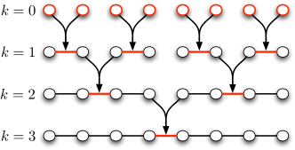
Figure 1: The procedure to thermalize an 8-qubit chain. After thermalizing individual qubits at level $k=0$, we pair them up and merge them by adding the Hamiltonian that connects the two qubits. This procedure is then repeated recursively as we merge two already thermalized regions of size $2^{k}$ at level $k$ to obtain a thermalized chain of size $2^{k+1}$ at level $k+1$.

We implement the merging perturbatively. Assume that we are given access to copies of $\rho\propto e^{-\beta H}$ (from previous steps). The Hamiltonian $H$ corresponds to the halves to be merged, but the procedure is more general. We want to generate the state $\rho^{(1)}\propto e^{-\beta(H+h)}$, where $h$ corresponds to the link between the two halves. We will see how to generate (with high probability) the state $\rho^{(\epsilon)}\propto e^{-\beta(H+\epsilon h)}$. We then repeat the same process to produce the sequence

$$\rho=\rho^{(0)}\to\rho^{(\epsilon)}\to\rho^{(2\epsilon)}\to\cdots\to\rho^{(1)}\;.$$ (1)

Every transformation in the sequence has some probability of failure, in which case we restart. If all of the steps succeed, we approximate the state $\rho^{(1)}$ with an error of $\mathcal{O}(\epsilon)$. It is important to remark that all the errors in this paper are in the trace norm. That is, in this case, for input $\rho$, we build a state $\sigma$ such that $\|\sigma-\rho^{(1)}\|_{\mathrm{Tr\,}}\in\mathcal{O}(\epsilon)$.

               

Figure 2: The conjugation circuit. First the quantum phase estimation circuit (QPE) writes the energy onto an ancilla register. Then the unitary U rotates the second ancilla conditioned on the energy. We measure the second ancilla and restart if we do not obtain $|0\rangle$.

We update the state $\rho\propto e^{-\beta H}$ to $\rho^{(\epsilon)}\propto e^{-\beta(H+\epsilon h)}$, to first order in $\epsilon$, in two steps. The first step is probabilistic and updates the probabilities of the Gibbs state through post-selection. If it fails, we will be forced to restart, and this will be the dominant part for the cost of the algorithm. In the second step we update the eigenbasis to the eigenbasis of $\rho^{(\epsilon)}$. We now assume perfect phase estimation and perfect dephasing, and later account for the cost and errors of these operations.

The probabilistic transformation of the first step is a conjugation with $e^{-\epsilon\beta h/2}$, to first order in $\epsilon$. We assume that $h\geq 0$. We use phase estimation and post-selection as in Fig. 2. This is similar to the procedure in poulin_samplingthermal_2009 . The phase estimation is of the unitary $e^{2\pi iht}$, with $1/t>h\geq 0$. It implements the map $\sum_{a}P_{a}|tE_{a}\rangle\langle 0|$, where $P_{a}$ is a projection of the system onto the eigenspace of $h$ with energy $E_{a}$. This energy gets written in an ancilla register initialized to $|0\rangle$. We rotate a second ancilla to $(1-\epsilon\beta{E}_{a}/2)|0\rangle+\cdots|1\rangle$, conditioned on the value of the previous ancilla register (unitary $U$ in Fig. 2), to get the map $\sum_{a}(1-\epsilon\beta{E}_{a}/2)P_{a}|tE_{a}0\rangle\langle 00|+\cdots$. We then undo the phase estimation, obtaining the map

$$\sum_{a}(1-\epsilon\beta{E}_{a}/2)P_{a} |00\rangle\langle 00|+\cdots$$

$$=(1-\epsilon\beta h/2)|00\rangle\langle 00|+\cdots$$ (2)

Finally we measure the ancilla, and fail unless we obtain $|0\rangle$. We denote the result obtained by applying the above map to $\rho$ as

$$\rho_{\rm prob}\propto(1-\epsilon\beta h/2)\rho(1-\epsilon\beta h/2)\;.$$ (3)

The success probability is

$$p\geq 1-\epsilon\beta\|h\|\;.$$ (4)

It can be seen that the conjugation with $1-\epsilon\beta h/2$ of the previous paragraph updates all the probabilities of the eigenstates correctly to first order in $\epsilon$. It also implements the appropriate transformation for the degenerate subspaces of $\rho$. Next, we update the eigenbasis from $H$ to $H+\epsilon h$, using the adiabatic approximation. This approximation can be seen as a consequence of the Zeno effect, which can be achieved through measurements or dephasing childs_quantum_2002 ; boixo_quantum_2009 . Here we implement the Zeno effect directly. More specifically, we use pure dephasing in the eigenbasis of $H+\epsilon h$ (see boixo_quantum_2009 ).

Denote by $\{P_{k^{\epsilon}}\}$ the projectors on the eigenbasis of $H+\epsilon h$. For input $\rho$, the operation $\sum_{k^{\epsilon}}P_{k^{\epsilon}}\rho P_{k^{\epsilon}}$ is pure dephasing on this eigenbasis. To qualify the effect of dephasing on $\rho_{\rm prob}$, we start by writing the result of this ideal operation as boixo_quantum_2009

$$\sum_{k^{\epsilon}}P_{k^{\epsilon}}\rho_{\rm prob}P_{k^{\epsilon}}=\lim_{\sigma\to\infty}\int dt\,g_{\sigma}(t)U_{\epsilon}(t)\rho_{\rm prob}U_{\epsilon}^{\dagger}(t)\;,$$ (5)

where $g_{\sigma}$ is the density function of a Gaussian distribution with $0$ mean and standard deviation $\sigma$, and $U_{\epsilon}(t)=e^{-i(H+\epsilon h)t}$. This equality is easy to check directly. We now use a Dyson series to second order for the time evolution:

$$U_{\epsilon}(t) =U_{0}(t)-i\epsilon A(t)-\epsilon^{2}B(t)$$ (6)

$$U_{0}(t) =e^{-iHt}$$ (7)

$$A(t) =\int_{0}^{t}dt_{1}\,U_{0}(t-t_{1})hU_{0}(t_{1})$$ (8)

$$B(t) =\int_{0}^{t}dt_{1}\,\int_{0}^{t_{1}}dt_{2}\,U_{0}(t-t_{1})hU_{0}(t_{1}-t_{2})hU_{\epsilon}(t_{2})\;.$$

We then insert terms to first order in $\epsilon$ from Eq. (6) into Eq. (5). The second (and higher, after expanding further) order terms can all be bounded by $\mathcal{O}(\epsilon^{2}\|h\|^{2})$ in the trace-norm.

We want to compare the state obtained after the dephasing to $\rho^{(\epsilon)}$, to first order in $\epsilon$. With this goal, we use the Dyson series in imaginary time to expand $\rho^{(\epsilon)}$. In this expansion we need intermediate states $\rho(\tilde{\beta})=e^{-\tilde{\beta}H}/\mathcal{Z}$, where the partition function is always at inverse temperature $\beta$, $\mathcal{Z}=\mathrm{Tr\,}e^{-\beta H}$. We obtain, to second order,

$$\rho^{(\epsilon)} =\rho-\epsilon\int_{0}^{\beta}d\beta_{1}\,\rho(\beta-\beta_{1})h\rho(\beta_{1})$$ (9)

$$+ \epsilon^{2}\int_{0}^{\beta}\!d\beta_{1}\int_{0}^{\beta_{1}}d\beta_{2}\,\rho(\beta-\beta_{1})h\rho(\beta_{1}-\beta_{2})h\rho(\beta_{2}).$$

The second and higher order corrections can be bounded by $\mathcal{O}(\epsilon^{2}\beta^{2}\|h\|^{2})$ in trace-norm. We assume that $\beta\geq 1$, so this error dominates the error $\mathcal{O}(\epsilon^{2}\|h\|^{2})$ above.

We aim to obtain the first order expression in Eq. (9) with our procedure. The spectral decomposition of $\rho$ is $\sum_{k}p_{k}P_{k}$, where $P_{k}$ is the projector to the subspace spanned by eigenstates with eigenvalue $E_{k}$ of $H$, and $p_{k}=e^{-\beta E_{k}}/\mathcal{Z}$. The term proportional to $\epsilon$ in the expansion of $\rho^{(\epsilon)}$ in Eq. (9) can be rewritten in terms of these projectors, up to normalization, as:

$$-\epsilon\sum_{k}p_{k}\left(P_{k}hP_{k}+\sum_{l\neq k}\frac{P_{l}hP_{k}+P_{k}hP_{l}}{E_{l}-E_{k}}\right).$$ (10)

Finally, using $H=\sum_{k}E_{k}P_{k}$ in Eq. (5), with the expansion (6), gives the first order correction Eq. (10).

Until now, we were considering the behavior of our algorithm assuming perfect phase estimation and dephasing, which is not realistic. We now account for the effects of the errors inherent in the two parts of our perturbative Hamiltonian update algorithm when implemented using only dynamical evolution with the Hamiltonian $H+kh$ for $0\leq k\leq 1$ . We quantify the total cost in terms of the evolution time.

For the conjugation circuit, we use high precision phase estimation knill_optimal_2007 ; somma_quantum_2008 ; poulin_samplingthermal_2009 ; chiang_quantum_2010 . The cost (evolution time with $h$), for accuracy $\delta$ and error $\varepsilon$, scales as $\mathcal{O}(\mathrm{log}(1/\varepsilon)/\delta)$. This implements the transformation

$$\sum_{a}P_{a}\otimes\Bigg{(}\Bigg{(}\sum_{\pm}c_{a}^{\pm}|tE_{a}^{\pm}\rangle+q_{a}|\xi_{a}\rangle\Bigg{)}\langle 0|\Bigg{)}\;,$$ (11)

with $t|E_{a}-E_{a}^{\pm}|\leq\delta$ and $q_{a}\leq\varepsilon$. The $t$ is the evolution time of the unitary $e^{2\pi iht}$ used for the phase estimation, with $1/t\geq h\geq 0$ as above. The term $|\xi_{a}\rangle$ groups all the states of the ancilla register with a reading outside the goal accuracy $\delta$.

First consider the effect of the error term $\sum_{a}q_{a}P_{a}|\xi_{a}\rangle$. All the manipulations conserve the projectors $P_{a}$ and do not increase the norm of $|\xi_{a}\rangle$. Therefore, the final error due to these terms, on input $\sigma$, can be bounded with terms like $\|\sum_{a}q_{a}P_{a}\sigma\|_{\rm tr}\leq\varepsilon$. The final error can increase as a result of the normalization when projecting onto the post-selected state, if the preparation is successful. We will see that this effect is negligible. We then rotate a second ancilla and undo the phase estimation to obtain an approximate version of the conjugation unitary in Eq. (Preparing thermal states of quantum systems by dimension reduction). The undo of the phase estimation incurs in an error bounded by $\mathcal{O}(\epsilon\beta\delta)$ in the trace norm, and the rest of the errors are $\mathcal{O}(\varepsilon)$ as before. If we choose $\varepsilon$ and $\epsilon\beta\delta$ to be $\mathcal{O}(\epsilon^{2}\beta^{2}\|h\|^{2})$, we can implement the map in Eq. (3) with the same probability (4) as before, trace norm error $\mathcal{O}(\epsilon^{2}\beta^{2}\|h\|^{2})$, and cost (evolution time)

$$\mathcal{O}\left(\mathrm{log}(1/(\epsilon\beta\|h\|))/(\epsilon\beta\|h\|^{2})\right).$$ (12)

Finally, we deal with the errors related to imperfect dephasing. Irrespective of the implementation of dephasing, imperfect accuracy in the dephasing results in an operation where only phases between eigenstates with relative gap bigger than some bound $\zeta$ are suppressed. This is modeled by the operation

$$\sigma\to\sum_{j^{\epsilon},k^{\epsilon}:|E^{\epsilon}_{k}-E^{\epsilon}_{j}|\leq\zeta}P_{k^{\epsilon}}\sigma P_{j^{\epsilon}}$$ (13)

(cf. Eq. (5)). We obtain imperfect dephasing if we choose the standard deviation of the Gaussian in Eq. (5) to be $\sigma=\mathcal{O}(1/\zeta)$, instead of (approaching) infinity .

We analyze the effect of imperfect dephasing errors by the following purely formal mathematical procedure. For a given Hamiltonian $H+\epsilon h$, we define the Hamiltonian $\tilde{H}$ which is similar to $H+\epsilon h$, but such that all the gaps are at least $\zeta$. We do this by increasing the degeneracy: we group all eigenvalues in bins with relative gap $\zeta$. The imperfect dephasing (or accuracy $\zeta$) would be fundamentally exact if the target Hamiltonian was $\tilde{H}$, because all the gaps would be bigger than the accuracy. Let $\chi=\tilde{H}-(H+\epsilon h)$, with $\|\chi\|\leq\zeta$ in operator norm.

By an expansion similar to that of Eq. (9) we can write $\rho^{(\epsilon)}=\tilde{\rho}^{(\epsilon)}+\mathcal{O}(\beta\zeta)$, where $\tilde{\rho}^{(\epsilon)}=e^{-\beta\tilde{H}}/\mathrm{Tr\,}e^{-\beta\tilde{H}}$ and the bound is, as always, in the trace norm . Similarly, we can write $U_{\epsilon}(t)$ in terms of $\tilde{U}_{\epsilon}(t)=e^{-i\tilde{H}t}$ and $\chi$ using Dyson series. Plugging these expressions into Eq. (5) with $\sigma=c/\zeta$ for a constant $c=\mathcal{O}(\mathrm{log}(1/\varepsilon))$, we get

$$\int dt\,g_{c/\zeta}(t)U_{\epsilon}(t)\rho_{\rm prob}U_{\epsilon}^{\dagger}(t)=\rho^{(\epsilon)}+\mathcal{O}(\beta\zeta)\;,$$ (14)

where $g_{c/\zeta}$ is a Gaussian with standard deviation $c/\zeta$. Now choosing $\zeta=\epsilon^{2}\beta\|h\|^{2}$ we see that we can transform $\rho$ to $\rho^{(\epsilon)}$ with the probability of Eq. (4), trace norm error $\mathcal{O}(\epsilon^{2}\beta^{2}\|h\|^{2})$, and cost (evolution time)

$$\mathcal{O}(\mathrm{log}(1/(\epsilon\beta\|h\|))/(\epsilon^{2}\beta\|h\|^{2}))\;.$$ (15)

We can merge two regions already thermalized into one large thermal region with the two subroutines just described using a sequence of small perturbative steps (see Eq. (1)). Each step is successful with the probability given in Eq. (4). The average number of steps until we generate a complete sequence without failures is $\langle m\rangle\in\mathcal{O}(e^{\beta\|h\|})$ . Each time that we fail we need to produce two new thermal regions to be merged. The average number of failures is $\langle\alpha\rangle\in\mathcal{O}(e^{\beta\|h\|})$.

Now we analyze the average number of steps $\langle\tau(k)\rangle$ required to prepare a thermalized chain of length $2^{k}$ at level $k$ (see Fig. 1). Since $\alpha$ and $\tau(k-1)$ are independent random variables, the expectation value of $\tau(k)$ is

$$\langle\tau(k)\rangle=2\langle\alpha\rangle\langle\tau(k-1)\rangle+\langle m\rangle\;.$$ (16)

This gives $\langle\tau(\mathrm{log}N)\rangle\in\mathcal{O}(\mathrm{exp}((\beta\|h\|+\mathrm{log}2)\mathrm{log}N))$. Similarly, the total error is $\mathcal{O}(N\epsilon\beta^{2}\|h\|^{2})$. If we choose $\epsilon$ = $\bar{\epsilon}/(N\beta^{2}\|h\|^{2})$, we get a total error of $\mathcal{O}(\bar{\epsilon})$ in trace-norm. Finally, using Eq. (15) for the evolution time of each step, we obtain the dominant contribution to the total evolution time $\beta N^{\beta\|h\|}/\bar{\epsilon}^{2}$.

We have presented an algorithm that prepares a thermal state of a 1D quantum system in time polynomial in the system size and exponential in the inverse temperature (as required by the existence of QMA-complete ground state problems in 1D). This algorithm can be generalized into $D$ dimensions. At level $k$ of the recursion, we have built squares (for 2D) or cubes that are now merged. We do not get polynomial scaling with system size for $D>1$ because the intersection of two neighboring regions goes like $N^{D-1}$. Note that this is to be expected because there exist 2D ground states with constant gap that encode the solution to NP-complete problems. A careful analysis confirms that the time complexity is dominated by the operations at the top level, and the dominating factor is $\beta e^{2\beta\|h\|DN^{D-1}}/\bar{\epsilon}^{2}$. This is an exponential speedup from the known $\mathrm{exp}(O(N^{D}))$. The memory requeriments still scale with the number of sites of the model, $N^{D}$.

There are also several possible improvements to the scaling of this algorithm. If one is interested in thermalizing a classical system with a small quantum perturbation one can first solve for the classical part of the Hamiltonian. Then, one would only need to use projections for the quantum perturbation. Also, if one is interested in thermalizing a quantum system with short-ranged quantum correlations, one can also use belief propagation hastings_quantum_2007 ; leifer_quantum_2008 ; poulin_belief_2008 ; bilgin_coarse-grained_2010 to reduce the storage requirements from $\mathcal{O}(N)$ qubits to $\mathcal{O}(l\,\mathrm{log}(N))$, where $l$ is a constant related to the quantum correlation length. This can be done by tracing out parts of the blocks that do not share any entanglement with the boundary to be merged. The time complexity of the algorithm remains the same as before. Note that the cost (both in memory and time) of the classical algorithm of quantum belief propagation for 1D quantum systems is exponential in $l\sim 1/T$. This bound is only heuristic, and similar to hastings_solving_2006 .

- (1) R. P. Feynman, Int. J. Theor. Phys. 21, 467 (1982)
- (2) S. Lloyd, Science 273, 1073 (1996)
- (3) A. Y. Kitaev, A. H. Shen, and M. N. Vyalyi, Classical and Quantum Computation (Amer. Math. Soc., 2002) p. 272
- (4) J. Kempe, A. Kitaev, and O. Regev, SIAM J. Comput. 35, 1070 (2006)
- (5) R. Oliveira and B. M. Terhal, Quant. Inf, Comp. Vol. 8, No. 10, pp. 0900-0924 (2008)(2005)
- (6) D. Aharonov, D. Gottesman, S. Irani, and J. Kempe, Commun. Math. Phys. 287, 41 (2009)
- (7) N. Schuch, I. Cirac, and F. Verstraete, Phys. Rev. Lett. 100, 250501 (2008)
- (8) B. M. Terhal and D. P. DiVincenzo, Phys. Rev. A 61, 022301 (2000)
- (9) K. Temme and et al.(2009), arXiv:0911.3635
- (10) M. Cramer and J. Eisert, New Journal of Physics 12, 055020 (2010), arXiv:0911.2475 [quant-ph]
- (11) D. Poulin and P. Wocjan, Phys. Rev. Lett. 103, 220502 (2009)
- (12) M. Yung and et al.(2010), arXiv:1005.0020 [quant-ph]
- (13) M. B. Hastings, Phys. Rev. B 73, 085115 (2006)
- (14) A. M. Childs and et al., Phys. Rev. A 66, 032314 (2002)
- (15) S. Boixo, E. Knill, and R. D. Somma, QIC 9, 833 (2009)
- (16) E. Knill, G. Ortiz, and R. D. Somma, Phys. Rev. A 75, 012328 (2007)
- (17) R. D. Somma and et al., Phys. Rev. Lett. 101, 130504 (2008)
- (18) C. Chiang and P. Wocjan(2010), arXiv:1001.1130
- (19) We can truncate the tails of the Gaussian distribution to ensure a worst time cost of the order of the average cost, and the resulting error is already dominated by the imperfect dephasing.
- (20) An analogous bound holds between and the Gibbs state of . We also need a bound on the difference between the partition functions of and , which can be found in poulin_samplingthermal_2009
- (21) This is also known from the theory of success runs. We give the average cost, but the tail has an exponential decay rate, so the worst case cost is similar (see, for instance balakrishnan_runs_2001 ).
- (22) M. B. Hastings, Phys. Rev. B 76, 201102 (2007)
- (23) M. Leifer and D. Poulin, Ann. Phys. 323, 1899 (2008)
- (24) D. Poulin and E. Bilgin, Phys. Rev. A 77, 052318 (2008)
- (25) E. Bilgin and D. Poulin, Phys. Rev. B 81, 054106 (2010)
- (26) N. Balakrishnan and M. V. Koutras, Runs and Scans with Applications, 1st ed. (Wiley-Interscience, 2001)