Superheating field of superconductors within Ginzburg-Landau theory

Abstract

We study the superheating field of a bulk superconductor within Ginzburg-Landau theory, which is valid near the critical temperature. We calculate, as functions of the Ginzburg-Landau parameter $\kappa$, the superheating field $H_{\mathrm{sh}}$ and the critical momentum $k_{c}$ characterizing the wavelength of the instability of the Meissner state to flux penetration. By mapping the two-dimensional linear stability theory into a one-dimensional eigenfunction problem for an ordinary differential equation, we solve the problem numerically. We demonstrate agreement between the numerics and analytics, and show convergence to the known results at both small and large $\kappa$. We discuss the implications of the results for superconducting RF cavities used in particle accelerators.

I Introduction

One of the primary features of superconductivity is the Meissner effect — the expulsion of a weak magnetic field from a bulk superconducting material Tinkham2004 . For sufficiently large magnetic fields, the Meissner state becomes unstable, and the system undergoes a phase transition. The exact nature of the transition depends on the so-called Ginzburg-Landau parameter, $\kappa=\lambda/\xi$, where $\lambda$ is the London penetration depth and $\xi$ the superconducting coherence length. Type I superconductors, characterized by small $\kappa$, transition from the Meissner state into a normal metal state for magnetic fields above the thermodynamic critical field, $H_{c}$. Type II superconductors, with larger $\kappa$, instead transition into a superconducting state with vortices above the first critical field $H_{c1}$. This state is stable up to a second critical field $H_{c2}$, above which the metal becomes normal. For any superconductor, however, the Meissner superconducting state is metastable, persisting up to the superheating field $H_{\mathrm{sh}}$, well above $H_{c}$ or $H_{c1}$ (for type I and II superconductors, respectively). The main goal of the present work is the calculation of $H_{\mathrm{sh}}$ as function of $\kappa$ for superconductors near the critical temperature $T_{c}$ where Ginzburg-Landau theory is applicable (we remind that within Ginzburg-Landau theory, the transition from type I to type II superconductors is at $\kappa=1/\sqrt{2}$).

The metastability of the Meissner state is of interest in the design of resonance RF cavities in particle accelerators, where $H_{\mathrm{sh}}$ places a fundamental limit on the maximum accelerating field Padamsee . As type II superconducting materials are being considered in cavity designs, a precise calculation of $H_{\mathrm{sh}}$ in this regime is of value. One must note, however, that operating temperatures of superconducting RF cavities are well below the critical temperature $T_{c}$ and that at these low temperatures Ginzburg-Landau theory is not quantitatively valid. The numerical techniques developed here are also being used within the Eilenberger formalism to address these lower temperatures inprep . Using this formalism, the limit $\kappa\to\infty$ was studied in Ref. Catelani2008 for arbitrary temperature.

Much work has already been done in calculating the superheating field within Ginzburg-Landau theory Gennes1965 ; Galaiko1966 ; Kramer1968 ; Kramer1973 ; Fink ; Christiansen ; Chapman1995 ; Dolgert1996 . The problem is formulated as follows: the superconductor occupies a half space with a magnetic field applied parallel to the surface. The order parameter and vector potential are functions of the distance from the surface and can be found by solving a boundary value problem of ordinary differential equations. The superheating field is then the largest magnetic field for which the corresponding solution is a local minimum of the free energy. For small values of $\kappa$, the superheating field corresponds to the largest magnetic field for which a nontrivial solution to the Ginzburg-Landau equations exist Dolgert1996 , as the instability does not break translational invariance. However, as $\kappa$ increases the one-dimensional solution is unstable to two-dimensional perturbations, resulting in a lower estimate of $H_{\mathrm{sh}}$ as first shown in Ref. Galaiko1966 . The task at hand is to find which perturbations destroy the Meissner state and at which value of the applied magnetic field they first become unstable.

The calculation of $H_{\mathrm{sh}}$ is therefore a linear stability analysis of the coupled system of superconducting order parameter and vector potential. For a given configuration, we study its stability to arbitrary two-dimensional perturbations by considering the second variation of the free energy: if the second variation is positive definite for all possible perturbations then the solution is (meta)stable. The second variation can be expressed as a Hermitian operator acting on the perturbations, so it is sufficient to show that the eigenvalues of this operator are all positive. By expanding the perturbations in Fourier modes parallel to the surface, the eigenvalue problem can once again be translated into a boundary value problem of an ordinary differential equation. The eigenvalues now depend upon the wave-number of the Fourier mode, but can otherwise be solved in the same way as the Ginzburg-Landau equations. The superheating field is then the largest applied magnetic field for which the smallest eigenvalue is positive for all Fourier modes.

The present stability analysis is more challenging than many such calculations, as the instability destabilizes an interface with a pre-existing depth-dependence of field and superconducting order parameter. As described above, we map the partial differential equation for the unstable mode into an eigenvalue analysis for a family of one-dimensional ordinary differential equations (as originally suggested, but not implemented, in Ref. Kramer1968 ). This technique could be useful in a variety of other linear stability calculations Brower ; Boden ; Ben-Jacob , replacing thin interface approximations with a microscopic depth-dependent treatment of the destabilizing interface.

The paper is organized as follows: in the next section we present the Ginzburg-Landau free energy and the differential equations to be studied for the stability analysis. In Sec. III we give some details about the numerical calculations and our main results. In Sec. IV we discuss the implications of the results for accelerator cavity design and outline future research directions. In Appendices we derive analytic formulas, valid at large $\kappa$, which we compare against the numerics.

II Ginzburg-Landau theory and stability analysis

The Ginzburg-Landau free energy for a superconductor occupying the half space $x>0$ in terms of the magnitude of the superconducting order parameter $f$ and the gauge-invariant vector potential $\mathbf{q}$ is given by

$$\mathcal{F}[f,\mathbf{q}] = \int_{x>0}d^{3}r\Big{\{}\xi^{2}(\nabla f)^{2}+\frac{1}{2}(1-f^{2})^{2}$$ (1)

$$+f^{2}\mathbf{q}^{2}+(\mathbf{H}_{a}-\lambda\nabla\times\mathbf{q})^{2}\Big{\}},$$

where $\mathbf{H}_{a}$ is the applied magnetic field (in units of $\sqrt{2}H_{c}$), $\xi$ is the Ginzburg-Landau coherence length, and $\lambda$ is the penetration depth. Note that after choosing the unit of length, the only remaining free parameter in the theory is the ratio of these two characteristic length scales, the Ginzburg-Landau parameter $\kappa=\lambda/\xi$. The magnetic field inside of the superconductor is given by $\mathbf{H}=\lambda\nabla\times\mathbf{q}$.

We take the applied field to be oriented along the $z$-axis $\mathbf{H}_{a}=(0,0,H_{a})$, and the order parameter $f=f(x)$ to depend only on the distance from the superconductor’s surface. We have assumed that the order parameter is real and further parametrize the vector potential as $\mathbf{q}=(0,q(x),0)$, which fixes the gauge. The Ginzburg-Landau equations that extremize $\mathcal{F}$ with respect to $f$ and $\mathbf{q}$ are

$$\begin{split}&\xi^{2}f^{\prime\prime}-q^{2}f+f-f^{3}=0,\\ &\lambda^{2}q^{\prime\prime}-f^{2}q=0,\end{split}$$ (2)

and with our choices $H=\lambda q^{\prime}$. Hereafter we use primes to denote derivatives with respect to $x$.

The boundary conditions at the surface derive from the requirement that the magnetic field be continuous, $q^{\prime}(0)=H_{a}/\lambda$, and that no current passes through the boundary, $f^{\prime}(0)=0$. We also require that infinitely far from the surface the sample is completely superconducting with no magnetic field, giving us $f(x)\rightarrow 1$ and $q(x)\rightarrow 0$ as $x\rightarrow\infty$. In the limits $\kappa\to 0$ and $\kappa\to\infty$, Eqs. (2) can be explicitly solved perturbatively, see Ref. Dolgert1996 and Appendix A, respectively. For arbitrary $\kappa$ they can be solved numerically via a relaxation method, as we discuss in Sec. III.

For a given solution $(f,\mathbf{q})$ we consider the second variation of $\mathcal{F}$ associated with small perturbations $f\rightarrow f+\delta f$ and $\mathbf{q}\rightarrow\mathbf{q}+\delta\mathbf{q}$ given by

$$\delta^{2}\mathcal{F} = \int_{x>0}d^{3}r\Big{\{}\xi^{2}(\nabla\delta f)^{2}+4f\delta f\mathbf{q}\cdot\delta\mathbf{q}+f^{2}\delta\mathbf{q}^{2}$$ (3)

$$(3f^{2}+\mathbf{q}^{2}-1)\delta f^{2}+\lambda^{2}(\nabla\times\delta\mathbf{q})^{2}\Big{\}}.$$

If the expression in Eq. (3) is positive for all possible perturbations, then the solution is stable. Since our solution $(f,\delta\mathbf{q})$ depends only on the distance from the boundary (and is therefore translationally invariant along the $y$ and $z$ directions), we can expand the perturbation in Fourier modes parallel to the surface. As shown in Ref. Kramer1968 , we can restrict our attention to perturbations independent of $z$ and write

$$\begin{split}\delta f(x,y)&=\delta\tilde{f}(x)\cos ky,\\ \delta\mathbf{q}(x,y)&=(\delta\tilde{q}_{x}\sin ky,\delta\tilde{q}_{y}\cos ky,0),\end{split}$$ (4)

where $k$ is the wave-number of the Fourier mode. The remaining Fourier components (corresponding to replacing $\cos\to\sin$ and vice-versa in Eq. 4) are redundent as they decouple from those given in Eq. 4 and satisfy the same differential equations derived below.

After substituting into the expression (3) for the second variation and integrating by parts, we arrive at

$$\delta^{2}\mathcal{F}=\int_{0}^{\infty}dx\left(\begin{array}[]{ccc}\delta\tilde{f}&\delta\tilde{q}_{y}&\delta\tilde{q}_{x}\end{array}\right)\left(\begin{array}[]{ccc}-\xi^{2}\frac{d^{2}}{dx^{2}}+q^{2}+3f^{2}+\xi^{2}k^{2}-1&2fq&0\\ 2fq&-\lambda^{2}\frac{d^{2}}{dx^{2}}+f^{2}&-\lambda^{2}k\frac{d}{dx}\\ 0&\lambda^{2}k\frac{d}{dx}&f^{2}+\lambda^{2}k^{2}\end{array}\right)\left(\begin{array}[]{c}\delta\tilde{f}\\ \delta\tilde{q}_{y}\\ \delta\tilde{q}_{x}\end{array}\right).$$ (5)

The matrix operator in Eq. (5) is self-adjoint, and the second variation will be positive definite if its eigenvalues are all positive. In the eigenvalue equations for this operator, the function $\delta\tilde{q}_{x}$ can be solved for algebraically. The resulting differential equations for $\delta\tilde{f}$ and $\delta\tilde{q}_{y}$ are

$$-\xi^{2}\delta\tilde{f}^{\prime\prime}+(3f^{2}+q^{2}-1+\xi^{2}k^{2})\delta\tilde{f}+2fq\delta\tilde{q}_{y} = E\delta\tilde{f},$$

and

$$-\lambda^{2}\frac{d}{dx}\left[\frac{f^{2}-E}{f^{2}+\lambda^{2}k^{2}-E}\delta\tilde{q}_{y}^{\prime}\right]+f^{2}\delta\tilde{q}_{y}+2fq\delta\tilde{f}=E\delta\tilde{q}_{y},$$ (7)

where $E$ is the stability eigenvalue. Note that by decomposing in Fourier modes, we have transformed the two-dimensional problem into a one-dimensional eigenvalue problem. Numerically, it can be solved by the same relaxation method as the Ginzburg-Landau equations – see Sec. III. The boundary conditions associated with the eigenvalue equations derive from the same physical requirements previously discussed: we require $\delta\tilde{f}^{\prime}(0)=0$, since no current may flow through the boundary, and $\delta\tilde{q}_{y}^{\prime}(0)=0$, since the magnetic field must remain continuous. Additionally, we require $\delta\tilde{f}(x)\rightarrow 0$ and $\delta\tilde{q}_{y}(x)\rightarrow 0$ as $x\rightarrow\infty$. There is also an arbitrary overall normalization, which we fix by requiring $\delta\tilde{f}(0)=1$.

The stability eigenvalue will depend on the solution of the Ginzburg-Landau equations, i.e., the applied magnetic field $H_{a}$, and the Fourier mode $k$ under consideration. The problem at hand is to find the applied magnetic field and Fourier mode for which the smallest eigenvalue first becomes negative, which is the case if the following two conditions hold:

$$E=0\,,\qquad\quad\frac{dE}{dk}=0.$$ (8)

The value of the magnetic field at which these conditions are met is the superheating field $H_{\mathrm{sh}}$, and the corresponding wave-number is known as the critical momentum $k_{c}$. In the next section we discuss in more detail the numerical approach used to calculate these two quantities.

III Numerical Results

As explained in the previous section, the calculation of the superheating field comprises two main steps: (1) solving the Ginzburg-Landau equations (2) and (2) solving the eigenvalue problem (LABEL:eq:eigen1)-(7) with conditions (8). To solve these equations we employ a relaxation method. The basic scheme is to replace the ordinary differential equations with a set of finite difference equations on a grid. From an initial guess to the solution, the method iterates using Newton’s method to relax to the true solution Press2007 . The grid is chosen with a high density of points near the boundary, with the density diminishing approximately as the inverse distance from the boundary. This is similar to the scheme used by Dolgert et al. Dolgert1996 to solve the Ginzburg-Landau equations for type I superconductors.

For $\kappa$ near the type I/II transition, the relaxation method typically converges without much difficulty. In the limiting cases that $\kappa$ becomes either very large or small, however, the grid spacing must be chosen with care to achieve convergence. The eigenfunction equations are particularly sensitive to the grid choice. This is not surprising, since in either limit there are two well-separated length scales. For example, using units $\lambda=1$ and $\xi=1/\kappa$, we find that a grid with density

$$\rho(x)=\frac{150\kappa}{1+25\kappa\\ x}$$ (9)

leads to convergence for $\kappa$ as high as 250. The grid points are then be generated recursively $x_{i+1}=x_{i}+1/\rho(x_{i})$ with $x_{0}=0$. We find that if the grid is not sufficiently sparse at large $x$, the relaxation method fails, presumably due to rouding errors. On the other hand if it is too sparse, the finite difference equations poorly approximate the true differential equation. Fortunately, the method converges quickly, allowing us to explore the density by trial and error, as we have done to get Eq. 9.

In solving Eq. 2, if a sufficiently large value for the applied magnetic field is used, there may not be a nonzero solution to the Ginzburg-Landau equations and the relaxation method will often fail to converge, indicating that the proposed $H_{a}$ is above the actual superheating field. In practice, therefore, it is more convenient to replace the boundary condition $q^{\prime}(0)=\lambda H_{a}$ with a condition on the value of the order parameter $f(0)=A$, which then implicitly defines the applied magnetic field as a function of $A$, $H_{a}(A)$. This has the advantage that $H_{a}(A)$ is a differentiable function of $A$, as is the stability eigenvalue, improving the speed and accuracy of the search for the superheating field. The drawback to this approach is that $H_{a}(A)$ is not single-valued, with an unstable branch of solutions as illustrated in Fig. 1. For the problem at hand, this turns out to be straightforward to address since we determine the stability of each solution in the second step. To achieve the conditions in Eq. (8), we vary both the Fourier mode, $k$, and the value of the order parameter at the surface $A$.

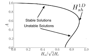
Figure 1: Solving for the 1-D Ginzburg-Landau superheating field. By fixing value of the order parameter at the surface, we implicitly define the applied magnetic field $H_{a}(A)$ at the surface. This definition produces a branch of unstable solutions, but guarantees that our equations will have a solution for all guesses of $A$. The “nose” of the curve occurs at the $H_{\mathrm{sh}}^{1D}$, the superheating field ignoring two-dimensional fluctuations, and is the largest $H_{a}$ for which a nontrivial solution to Eq. (2) can be found. This example was calculated for $\kappa=1$, and $H_{\mathrm{sh}}^{1D}\approx 0.9$.

The results of the procedure described above are summarized in Figs. 2-5, where we also compare them with analytical estimates which, for large values of $\kappa$, are derived in Appendices. In Fig. 2 we plot the numerically calculated superheating field as a function of $\kappa$ (solid line). The vertical line at $\kappa_{c}\simeq 1.1495$ separates the regimes of one-dimensional (1D, $k=0$) and two-dimensional (2D, $k\neq 0$) critical perturbations. We have checked the value of $\kappa_{c}$ both by assuming 2D perturbations and finding when their critical momentum goes to zero and by assuming 1D perturbation and finding when the coefficient of the term quadratic in momentum in the second variation of the free energy vanishes; these methods lead to the same value within our numerical accuracy of $10^{-4}$. Our value of $\kappa_{c}$ is higher than previous estimates, which ranged from 0.5 Kramer1968 to 1.10 Fink and 1.13($\pm$0.05) Christiansen . $\kappa_{c}$ is larger than the boundary $\kappa=1/\sqrt{2}$ separating type I from type II superconductors. Type II superconductors for which $\kappa<\kappa_{c}$ become unstable via a spatially uniform invasion of magnetic flux. Additionally, we find that superheated type II superconductors with $\kappa<0.9192$ can transition directly into the normal state since the corresponding $H_{\mathrm{sh}}$ is larger than the second critical field $H_{c2}$.

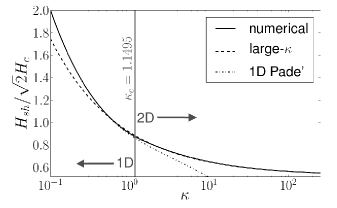
Figure 2: Numerically calculated $H_{\mathrm{sh}}$ and corresponding analytical approximations [Eqs. (10) and (11)] versus the Ginzburg-Landau parameter $\kappa$.

For $\kappa<\kappa_{c}$ the instability is due to 1D perturbations. In this regime, the Padé approximant

$$\frac{H_{\mathrm{sh}}(\kappa)}{\sqrt{2}H_{c}}\approx 2^{-3/4}\kappa^{-1/2}\frac{1+4.6825120\kappa+3.3478315\kappa^{2}}{1+4.0195994\kappa+1.0005712\kappa^{2}}$$ (10)

derived in Ref. Dolgert1996 (dot-dashed line) gives a good approximation to the actual $H_{\mathrm{sh}}$, with deviation of less than about 1.5 %. In the opposite case $\kappa>\kappa_{c}$, 2D perturbations are the cause of instability and the superheating field is approximately given by Christiansen (dashed line)

$$\frac{H_{\mathrm{sh}}(\kappa)}{\sqrt{2}H_{c}}\approx\frac{\sqrt{10}}{6}+\frac{0.3852}{\sqrt{\kappa}}.$$ (11)

Equation (11), derived in Appendix B, is also a good approximation, deviating at most about 1 % from the numerics. Therefore, our numerics show that the simple analytical formulas for $H_{\mathrm{sh}}$ in Eqs. (10) and (11) can be used to accurately estimate the superheating field for arbitrary value of the Ginzburg-Landau parameter, when used in their respective validity regions.

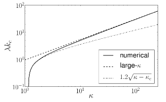
Figure 3: Comparison between the numerical and asymptotic critical momentum $k_{c}$, Eq. (13). The approximate behavior of $k_{c}$ near $\kappa_{c}$ (dot-dashed) is given in Eq. (12).

In Fig. 3 we show the numerical result for the critical momentum $k_{c}$ versus $\kappa$. We see that $k_{c}\to 0$ as $\kappa\to\kappa_{c}$ from above. Near $\kappa_{c}$, the behavior of $k_{c}$ is reminiscent of that of an order parameter near a second-order phase transition:

$$k_{c}\simeq 1.2\sqrt{\kappa-\kappa_{c}},$$ (12)

where the prefactor has been estimated by fitting the numerics. The dashed line is the asymptotic formula Christiansen (see also Appendix B)

$$\lambda k_{c}\approx 0.9558\kappa^{3/4}$$ (13)

which captures correctly the large-$\kappa$ behavior.

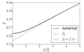
Figure 4: Profile of the order parameter at $H_{\mathrm{sh}}$ for $\kappa=50$ together with analytic approximations given in Eqs. (15) and (28).

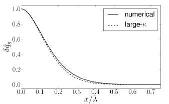
Figure 5: Numerical profile (solid line) of the critical perturbation $\delta\tilde{q}_{y}$ determining $H_{\mathrm{sh}}$ for $\kappa=50$ compared to the large-$\kappa$ perturbative result (dashed), Eq. (50).

In Fig. 4 we present a typical solution for the order parameter near the surface at $H=H_{\mathrm{sh}}$ for a large value of $\kappa$, along with the analytic approximations presented in Appendix A. The zeroth order approximation $f_{0}$, Eq. (15), fails near the surface, as it does not satisfy the boundary condition $f^{\prime}(0)=0$. On the other hand, including the first order correction in $1/\kappa$, Eq. (28), leads to excellent agreement with the numerics. Finally, in Fig. 5 we show a typical example of the depth dependence of the perturbation $\delta\tilde{q}_{y}$ at the critical point where the solution first becomes unstable. We find again good agreement between numerical and perturbative calculations.

It is interesting to compare the wavelength of the critical perturbation, $2\pi/k_{c}$, with the Abrikosov spacing $a$ for the arrangement of vortices at the superheating field: the naive expectation is that the initial flux penetrations represent nuclei for the final vortices. Kramer argues that this picture is incorrect since the initial flux penetrations do not have supercurrent singularities and do not carry a fluxoid quantum Kramer1968 .

We find the numerical discrepancies between the two lengths further support Kramer’s argument. In the weakly type-II regime ($\kappa\sim 1$), the initial flux penetration is from infinitely long wavelengths ($k_{c}=0$); in contrast, the final vortex state has a very high density, since $H_{\mathrm{sh}}\sim H_{c2}$ note1 . In the strongly type-II limit ($\kappa\rightarrow\infty$) both the inverse momentum and the Abrikosov spacing (evaluated at the superheating field) vanish, but at different rates, with $1/k_{c}\sim\kappa^{-3/4}$ while the Abrikosov spacing $a\sim\kappa^{-1/2}$ at $H_{\mathrm{sh}}$ note2 , see Fig. 6. These results suggest that there is no immediate connection between the initial penetration and the final vortex array. A dynamical simulation could explore the transition between the initial penetration and the final vortex state, similar to that done by Frahm et. al for the transition from the normal state to the vortex state Frahm1991 .

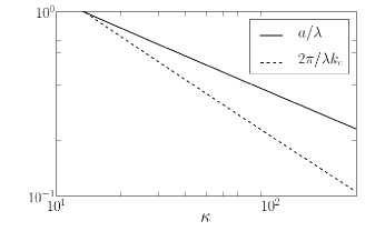
Figure 6: The wavelength of the critical perturbation ($2\pi/k_{c}$) and the Abrikosov vortex spacing ($a$) calculated at the superheating field both vanish at large $\kappa$, although the former diminishes much more quickly.

IV Summary and outlook

In this paper, we have numerically calculated within Ginzburg-Landau theory the superheating field $H_{\mathrm{sh}}$ of superconductors by mapping the linear stability threshold onto an eigenfunction problem, and we have shown that analytic approximations are in good agreement with the numerical results. The technique of mapping the linear stability problem onto a one-dimensional eigenfunction problem is potentially a useful technique, and we hope others find useful applications of the methods described here.

One of the primary motivations for this work is the application to RF cavities in particle accelerators, where the maximum accelerating field is limited by $H_{\mathrm{sh}}$. While the results presented here provide good estimates of $H_{\mathrm{sh}}$ for many materials of interest near the critical temperature $T_{c}$, we emphasize that the operating temperature of these cavities are typically well below $T_{c}$, where Ginzburg-Landau theory is not quantitatively accurate. The techniques presented here can be applied to Eilenberger theory to more accurately determine $H_{\mathrm{sh}}$ at low temperatures. The Eilenberger approach has already been used Catelani2008 to evaluate $H_{\mathrm{sh}}(T)$ at any temperature in the infinite $\kappa$ limit for clean superconductors, and work is in progress to address low temperatures for finite $\kappa$ inprep .

Appendix A Order parameter and vector potential in the large $\kappa$ limit

In this Appendix, we derive solutions to the Ginzburg-Landau equations Eq. (2) valid in the large-$\kappa$ limit. For convenience, we work in units $\lambda=1$, $\xi=1/\kappa$. As a first step, we consider the limit $\kappa\to\infty$. Then Eqs. 2 reduce to

$$\begin{split}q_{0}^{\prime\prime}&=f_{0}^{2}q_{0},\\ 0&=f_{0}\left(f_{0}^{2}-1+q_{0}^{2}\right),\end{split}$$ (14)

with solution Gennes1965

$$\begin{split}q_{0}(x)=-\frac{\sqrt{2}}{\cosh(x+\ell)},\\ f_{0}(x)=\sqrt{1-q_{0}^{2}(x)},\end{split}$$ (15)

where the parameter $\ell$ is determined by the field at the surface via

$$H_{a}=q_{0}^{\prime}(0)=\frac{\sqrt{2}\sinh\ell}{\cosh^{2}\ell}.$$ (16)

The above solution satisfies the boundary conditions at infinity, but it cannot satisfy the boundary condition for $f$ at the surface. An approximate solution, valid at finite but large $\kappa$, which satisfies all boundary conditions can be obtained by boundary layer theory. We follow the approach of Ref. Chapman1995 , so we only sketch the steps of the calculation. Note that away from the thermodynamic critical field, the scaling is different than that used in Ref. Chapman1995 : there the expansion is in powers of $\kappa^{-\alpha}$ and the inner variable is $X=\kappa^{\alpha}x$ with $\alpha=2/3$, here we use $\alpha=1$:

$$\begin{split}q&=q_{0}+\frac{1}{\kappa}q_{1}+\ldots\\ f&=f_{0}+\frac{1}{\kappa}f_{1}+\ldots\end{split}$$ (17)

Substituting into Eqs. (2), we find the following “outer layer” equations for $q_{1}$ and $f_{1}$:

$$\begin{split}q_{1}^{\prime\prime}&=2f_{0}f_{1}q_{0}+f_{0}^{2}q_{1},\\ 0&=f_{1}(3f_{0}^{2}-1+q_{0}^{2})+2f_{0}q_{0}q_{1}\end{split}$$ (18)

which have the simple solutions $f_{1}=q_{1}=0$. For the inner layer, we introduce the variable $X=\kappa x$ and find the equations

$$\begin{split}\tilde{f}_{0}^{\prime\prime}&=\tilde{f}_{0}\left(\tilde{f}_{0}^{2}-1+\tilde{q}_{0}^{2}\right),\\ \tilde{q}_{0}^{\prime\prime}&=0,\end{split}$$ (19)

and

$$\begin{split}\tilde{f}_{1}^{\prime\prime}&=\tilde{f}_{1}\left(3\tilde{f}_{0}^{2}-1+\tilde{q}_{0}^{2}\right)+2\tilde{f}_{0}\tilde{q}_{0}\tilde{q}_{1},\\ \tilde{q}_{1}^{\prime\prime}&=0,\end{split}$$ (20)

where we use tildes to denote functions of the inner variable $X$. Equations 19 have constant solutions

$$\tilde{q}_{0}=-b\,,\quad\tilde{f}_{0}=\sqrt{1-b^{2}},$$ (21)

while from the second of Eqs. (20) and the boundary conditions we get

$$\tilde{q}_{1}=H_{a}X\,.$$ (22)

Then the first of Eqs. (20) becomes

$$\tilde{f}_{1}^{\prime\prime}=2(1-b^{2})\tilde{f}_{1}-2b\sqrt{1-b^{2}}H_{a}X,$$ (23)

with solution

$$\tilde{f}_{1}=\frac{bH_{a}}{\sqrt{1-b^{2}}}X+Ae^{-\sqrt{2}\sqrt{1-b^{2}}X}+Be^{\sqrt{2}\sqrt{1-b^{2}}X}$$ (24)

with $A,B$ integration constants. Since $f$ tends to a constant far from the surface, we set $B=0$. Vanishing of the derivative at the surface then fixes

$$A=\frac{bH_{a}}{\sqrt{2}(1-b^{2})}$$ (25)

Next, we match the inner and outer solutions. Comparing Eqs. (15) and (21) we get

$$b=\frac{\sqrt{2}}{\cosh\ell}.$$ (26)

We can express $b$ in terms of the applied field using Eq. (16) to find

$$b=\sqrt{1-\sqrt{1-2H_{a}^{2}}}.$$ (27)

Then, since $f_{1}=q_{1}=0$, we need to compare the linear order expansion of Eqs. (15) at small $x$ with $\tilde{q}_{1}/\kappa$ and $\tilde{f}_{1}/\kappa$ at large $X=\kappa x$. Using Eqs. (16) and (26), we find that the inner and outer solutions match. Finally, the uniform approximate solution is

$$\begin{split}q(x)&=q_{0}(x),\\ f(x)&=\sqrt{1-q_{0}^{2}(x)}+\frac{1}{\kappa}\frac{bH_{a}}{\sqrt{2}(1-b^{2})}e^{-\sqrt{2}\sqrt{1-b^{2}}\kappa x}\end{split}$$ (28)

with corrections of order $1/\kappa^{2}$. In Fig. 4 we compare the second of Eq. (28) to numerics.

Appendix B Superheating field in the large-$\kappa$ limit

The calculation of the superheating field $H_{\mathrm{sh}}$ as a function of $\kappa$ for stability with respect to one-dimensional perturbations (i.e., $k=0$) can be found in Ref. Dolgert1996 for $\kappa\to 0$ and Ref. Chapman1995 for $\kappa\to\infty$. The latter calculation, however, is of little physical relevance, as the actual instability at sufficiently large $\kappa$ is due to two-dimensional perturbations. Here we present for completeness (albeit in a different form) Christiansen’s perturbative calculation Christiansen of the true superheating field $H_{\mathrm{sh}}(\kappa)$ for $\kappa\gg 1$.

Our starting point is the following expression for the “critical” second variation of the thermodynamic potential as functional of perturbations $\delta\tilde{f}$, $\delta\tilde{q}_{y}$, and momentum $k$ [see also Eq. (10) in Ref. Kramer1968 ]:

$$\begin{split}\delta^{2}\mathcal{F}=&\int_{0}^{\infty}\!\!dx\Big{\{}\left[3f^{2}+q^{2}-1+(k/\kappa)^{2}\right]\delta\tilde{f}^{2}+\kappa^{-2}\delta\tilde{f}^{\prime 2}\\ &\qquad+4fq\delta\tilde{f}\delta\tilde{q}_{y}+f^{2}\delta\tilde{q}_{y}^{2}+(f^{2}+k^{2})^{-1}f^{2}\delta\tilde{q^{\prime}}_{y}^{2}\Big{\}}\end{split}$$ (29)

It is straightforward to check that variation of this functional with respect to $f$ and $q_{y}$ leads to Eqs. (LABEL:eq:eigen1)-(7) with $E=0$ and rescaled units $\lambda=1$. Kramer estimated that the critical momentum $k\propto\sqrt{\kappa}$. While we will show that this is not the correct scaling, this form suggests to rescale lengths by $1/\sqrt{\kappa}$ by defining $x=w/\sqrt{\kappa}$:

$$\begin{split}\delta^{2}\mathcal{F}=&\int_{0}^{\infty}\!\frac{dw}{\sqrt{\kappa}}\Big{\{}\left[3f^{2}+q^{2}-1+(k/\kappa)^{2}\right]\delta\tilde{f}^{2}+\kappa^{-1}\delta\tilde{f}^{\prime 2}\\ &\qquad+4fq\delta\tilde{f}\delta\tilde{q_{y}}+f^{2}\delta\tilde{q}_{y}^{2}+(f^{2}+k^{2})^{-1}f^{2}\kappa\delta\tilde{q^{\prime}_{y}}^{2}\Big{\}}\end{split}$$ (30)

where now prime is derivative with respect to $w$. (Note that although $k$ has units of inverse length, it is momentum parallel to the surface, and therefore does not scale with $x$.)

Minimization with respect to $k$ leads to the equation

$$k\int\!dw\left[\frac{\delta\tilde{f}^{2}}{\kappa^{2}}-\frac{\kappa f^{2}}{(f^{2}+k^{2})^{2}}\delta\tilde{q}_{y}^{\prime 2}\right]=0$$ (31)

Assuming $k\gg 1$, we can neglect $f^{2}\leq 1$ in the denominator and find

$$k^{4}\int\!dw\,\delta\tilde{f}^{2}=\kappa^{3}\int\!dw\,f^{2}\delta\tilde{q}_{y}^{\prime 2}$$ (32)

which shows that (if our length rescaling is correct) the proper scaling for the critical momentum is $k\propto\kappa^{3/4}$. If this is true, then $(k/\kappa)^{2}\propto 1/\sqrt{\kappa}$ and $\kappa/k^{2}\propto 1/\sqrt{\kappa}$, which shows that the next to leading order terms in curly brackets in Eq. (30) are proportional to $1/\sqrt{\kappa}$. Therefore, terms of order $1/\kappa$ can be neglected and, in particular, we can neglect $\kappa^{-1}\delta\tilde{f}^{\prime 2}$ and use everywhere the lowest order solution for $f$ and $q$, Eq. (15). Hence the approximate functional in the large-$\kappa$ limit is

$$\begin{split}\delta^{2}\mathcal{F}\simeq&\frac{1}{\sqrt{\kappa}}\int_{0}^{\infty}\!\!dw\Big{\{}\left[2f_{0}^{2}+(k/\kappa)^{2}\right]\delta\tilde{f}^{2}\\ &\quad+4f_{0}q_{0}\delta\tilde{f}\delta\tilde{q}_{y}+f_{0}^{2}\delta\tilde{q}_{y}^{2}+k^{-2}f_{0}^{2}\kappa\delta\tilde{q}_{y}^{\prime 2}\Big{\}}.\end{split}$$ (33)

By minimizing Eq. (33) with respect to $\delta\tilde{f}$, we find

$$\left[2f_{0}^{2}+(k/\kappa)^{2}\right]\delta\tilde{f}=-2f_{0}q_{0}\delta\tilde{q}_{y},$$ (34)

and solving for $\delta\tilde{f}$

$$\delta\tilde{f}=-\frac{2f_{0}q_{0}\delta\tilde{q}_{y}}{2f_{0}^{2}+(k/\kappa)^{2}}\simeq-\frac{q_{0}\delta\tilde{q}_{y}}{f_{0}}+\left(\frac{k}{\kappa}\right)^{2}\frac{q_{0}\delta\tilde{q}_{y}}{2f_{0}^{3}}$$ (35)

where in the last step we kept only the leading and the next to leading order terms. Substituting back into Eq. (33) gives

$$\begin{split}\delta^{2}\mathcal{F}=&\int_{0}^{\infty}\!\frac{dw}{\sqrt{\kappa}}\bigg{[}\left(1-3q_{0}^{2}\right)\delta\tilde{q}_{y}^{2}\\ &+\left(\frac{k}{\kappa}\right)^{2}\frac{q_{0}^{2}}{f_{0}^{2}}\delta\tilde{q}_{y}^{2}+\frac{\kappa}{k^{2}}f_{0}^{2}\delta\tilde{q}_{y}^{\prime 2}\bigg{]}\end{split}$$ (36)

The first term in square brackets is the leading term. Neglecting the other terms, since $q_{0}^{2}$ is monotonically decreasing function of $w$ the variation $q_{y}$ that minimizes the functional is a $\delta$-function at the surface. Then the condition for the metastability is

$$1-3q_{0}^{2}(0)=0.$$ (37)

Using Eq. (15) we obtain

$$\cosh\ell=\sqrt{6}\,,\quad\sinh\ell=\sqrt{5}$$ (38)

and substituting into Eq. (16)

$$H_{\mathrm{sh}}^{\infty}=\frac{\sqrt{10}}{6}$$ (39)

To calculate the large-$\kappa$ correction, we expand the function $q_{0}(w)$ in the first term in square brackets in Eq. (36) to linear order, while $q_{0}$ and $f_{0}$ in the subleading terms can be simply evaluated at the surface. Setting

$$\ell\simeq\mathrm{arccosh}\sqrt{6}-\frac{c}{\sqrt{\kappa}},$$ (40)

$$k=\left(\frac{5}{6}\right)^{1/4}\tilde{k}\kappa^{3/4},$$ (41)

and using Eq. (16) we find

$$\begin{split}\delta^{2}\mathcal{F}=2\sqrt{\frac{5}{6}}\int_{0}^{\infty}\!\frac{dw}{\kappa}\bigg{[}\left(-c+w+\frac{1}{4}\tilde{k}^{2}\right)\delta\tilde{q}_{y}^{2}+\frac{2}{5\tilde{k}^{2}}\delta\tilde{q}_{y}^{\prime 2}\bigg{]}\end{split}$$ (42)

The variational equation for $\delta\tilde{q}_{y}$ derived from this functional has as solution the Airy function

$$\delta\tilde{q}_{y}(w)=\mathrm{Ai}\left[\left(\frac{5\tilde{k}^{2}}{2}\right)^{1/3}\left(w-c+\frac{1}{4}\tilde{k}^{2}\right)\right]$$ (43)

Imposing the boundary condition $\delta\tilde{q}_{y}^{\prime}(0)=0$, we find that for a given $\tilde{k}$ the lowest possible $c$ is

$$c=z_{0}\left(\frac{5\tilde{k}^{2}}{2}\right)^{-1/3}+\frac{1}{4}\tilde{k}^{2},$$ (44)

where

$$z_{0}\approx 1.018793$$ (45)

is the smallest number satisfying $\mathrm{Ai}^{\prime}(-z_{0})=0$. Finally minimizing $c$ with respect to $\tilde{k}$ we find

$$\tilde{k}=\left(\frac{4}{3}z_{0}\right)^{3/8}\left(\frac{2}{5}\right)^{1/8}$$ (46)

and

$$c=\left(\frac{2}{5}\right)^{1/4}\left(\frac{4}{3}z_{0}\right)^{3/4}.$$ (47)

Substituting Eq. (40) into Eq. (16) we obtain

$$H_{\mathrm{sh}}=\frac{\sqrt{10}}{6}+\frac{2c}{3\sqrt{3\kappa}}\approx\frac{\sqrt{10}}{6}+\frac{0.3852}{\sqrt{\kappa}}$$ (48)

and from Eqs. (41), (45), and (46)

$$k = \left(\frac{160}{243}\right)^{1/8}z_{0}^{3/8}\kappa^{3/4}$$ (49)

$$\approx 0.9558\kappa^{3/4}.$$

These results agree with those of Ref. Christiansen . We compare these two formulas with numerics in Figs. 2 and 3, respectively.

Finally, fixing the arbitrary normalization of the perturbation by requiring $\delta\tilde{q}_{y}(0)=0$, using Eqs. (43)-(47), and restoring dimensions we find

$$\delta\tilde{q}_{y}(x)=\mathrm{Ai}\left[\left(\frac{10}{3}z_{0}\right)^{1/4}\frac{\sqrt{\kappa}x}{\lambda}-z_{0}\right]\bigg{/}\mathrm{Ai}[-z_{0}],$$ (50)

which shows that the “penetration depth” of the perturbation is of the order of the geometric average of coherence length and magnetic field penetration depth. This functional form is plotted in Fig. 5 for $\kappa=50$ along with the numerically calculated $\delta\tilde{q}_{y}$.

References

- (1) M. Tinkham, Introduction to Superconductivity, 2nd ed. (McGraw-Hill, New York, 1996).
- (2) H. Padamsee, K. W. Shepard, and R. Sundelin, Annu. Rev. Nucl. Part. Sci. 43, 635 (1993); H. Padamsee, Supercond. Sci. Technol. 14, R28 (2001).
- (3) M. K. Transtrum. G. Catelani, and J. P. Sethna, in preparation
- (4) G. Catelani and J. P. Sethna, Phys. Rev. B 78, 224509 (2008).
- (5) L. Kramer, Phys. Rev. 170, 475 (1968).
- (6) P. G. de Gennes, Solid State Commun. 3, 127 (1965).
- (7) V. P. Galaiko, Zh. Eksp. Teor. Fiz. 50, 717 (1966) [Sov. Phys. JETP 23, 475(1966)].
- (8) L. Kramer, Z. Phys. 259, 333 (1973).
- (9) H. J. Fink and A. G. Presson, Phys. Rev. 182, 498 (1969).
- (10) P. V. Christiansen, Solid State Commun. 7, 727 (1969).
- (11) S. J. Chapman, SIAM J. Appl. Math. 55, 1233 (1995).
- (12) A. J. Dolgert, S. J. Di Bartolo, and A. T. Dorsey, Phys. Rev. B 53, 5650 (1996); Phys. Rev. B 56, 2883 (1997).
- (13) R. C. Brower, D. A. Kessler, J. Koplik, and H. Levine, Phys. Rev. Lett. 51, 1111 (1983).
- (14) E. Bodenschatz, W. Pesch, and G. Ahlers, Annu. Rev. Fluid Mech. 32, 709 (2000).
- (15) E. Ben-Jacob, N. Goldenfeld, J. Langer, and G. Schön, Phys. Rev. Lett. 51, 1930 (1983); Phys. Rev. A 29, 330 (1984).
- (16) W. Press, S. A. Teukolsky, W. T. Vetterling, and B. P. Flannery, Numerical Recipes: the art of scientific computing, (Cambridge University Press, 2007).
- (17) We remind that in our units ; see, e.g., A. L. Fetter and P. C. Hohenber, in Superconductivity, edited by R. D. Parks (Dekker, New York, 1969), Chap. 14.
- (18) The vortex spacing is related to the induction as , and at intermediate fields such that , – see the reference in the previous footnote. Since at large the superheating field tends to a constant, we find .
- (19) H. Frahm, S. Ullah, and A. T. Dorsey, Phys. Rev. Lett. 66, 3067 (1991).