Only the Lonely: H I Imaging of Void Galaxies

Abstract

Void galaxies, residing within the deepest underdensities of the Cosmic Web, present an ideal population for the study of galaxy formation and evolution in an environment undisturbed by the complex processes modifying galaxies in clusters and groups, as well as provide an observational test for theories of cosmological structure formation. We have completed a pilot survey for the H i imaging aspects of a new Void Galaxy Survey (VGS), imaging 15 void galaxies in H i in local ($d<100$ Mpc) voids. H i masses range from $3.5\times 10^{8}$ to $3.8\times 10^{9}M_{\odot}$, with one nondetection with an upper limit of $2.1\times 10^{8}M_{\odot}$. Our galaxies were selected using a structural and geometric technique to produce a sample that is purely environmentally selected and uniformly represents the void galaxy population. In addition, we use a powerful new backend of the Westerbork Synthesis Radio Telescope that allows us to probe a large volume around each targeted galaxy, simultaneously providing an environmentally constrained sample of fore- and background control sample of galaxies while still resolving individual galaxy kinematics and detecting faint companions in H i. This small sample makes up a surprisingly interesting collection of perturbed and interacting galaxies, all with small stellar disks. Four galaxies have significantly perturbed H i disks, five have previously unidentified companions at distances ranging from 50 to 200 kpc, two are in interacting systems, and one was found to have a polar H i disk. Our initial findings suggest void galaxies are a gas-rich, dynamic population which present evidence of ongoing gas accretion, major and minor interactions, and filamentary alignment despite the surrounding underdense environment.

1 Introduction

With the prevalence of ever wider and deeper redshift surveys, from the second Center for Astrophysics Redshift Survey (Huchra et al., 1983) to the Sloan Digital Sky Survey (SDSS, York et al. 2000), we have refined our ability to identify the elongated filaments, sheetlike walls and dense compact clusters that compose the Cosmic Web (Zel’dovich, 1970; Klypin & Shandarin, 1983; de Lapparent et al., 1986; Bond et al., 1996; van de Weygaert & Bond, 2008). These structures surround voids, enormous regions $10-30h^{-1}$ Mpc in diameter that are largely devoid of galaxies and occupy most of the volume of the Universe (Gregory & Thompson 1978; Einasto et al. 1980; Kirshner et al. 1981; de Lapparent et al. 1986; Hoyle & Vogeley 2004; for a recent review see van de Weygaert & Platen 2009). Within these underdense – but not empty – regions, large galaxy redshift surveys have allowed us to distinguish an environmentally defined population of void galaxies residing in regions up to 10 times less dense than the cosmic mean. Largely unaffected by the complexities and processes modifying galaxies in high-density environments, these isolated void regions are expected to hold important clues to understanding the environmental influences on galaxy formation and evolution (Szomoru et al., 1996; Grogin & Geller, 2000; Corbin et al., 2005; Patiri et al., 2006b; Pustilnik et al., 2006; Wegner & Grogin, 2008; Stanonik et al., 2009). Additionally, the apparent underabundance of galaxies in the void regions may present a challenge for currently favored galaxy formation theories (Peebles, 2001; Mathis & White, 2002; Gottlöber et al., 2003; Furlanetto & Piran, 2006; Tinker & Conroy, 2009), while their distribution is expected to trace substructure within voids, tenuous features which are fossil remnants of the hierarchical buildup of the Cosmic Web (Dubinski et al., 1993; van de Weygaert & van Kampen, 1993; Popescu et al., 1997; Sheth & van de Weygaert, 2004; Patiri et al., 2006a; Tikhonov & Karachentsev, 2006).

Void galaxies appear to have a more youthful state of star formation. As a population, void galaxies are statistically bluer, have a later morphological type, and have higher specific star formation rates than galaxies in average density environments (Grogin & Geller, 1999, 2000; Rojas et al., 2004, 2005). Whether void galaxies are intrinsically different or whether their characteristics are simply due to the low mass bias of the galaxy luminosity function in low density regions is still an issue of discussion. Overall, the mean colors of the red and blue void galaxy populations, taken separately, are comparable to galaxies in average density environments at the same luminosity, though an excess of blue galaxies is apparent (Balogh et al., 2004; Patiri et al., 2006b). This suggests that in some respects the general underdensity of the environment has had little to no impact on their development, raising the question of to what extent the global ($\sim$20 Mpc) as opposed to local ($\sim$1 Mpc) environment shapes the formation and evolution of galaxies. Park et al. (2007) suggest that it is only the morphology and luminosity of void galaxies which is dependent on their environment, with all other statistical correlations stemming from these two key parameters. Interestingly, they and others find contradictory indications of a slight blueward shift of the blue cloud in voids at fixed luminosity (Blanton et al., 2005; von Benda-Beckmann & Müller, 2008). No such shift has been found for the red sequence of early type galaxies.

Less is known about the gas content of void galaxies. Szomoru et al. (1996) surveyed galaxies within the Boötes void with pointed observations of 24 IRAS selected galaxies, of which 16 were detected. Most of these galaxies are found to be gas-rich and disk-like, with many gas-rich companions, however more complete redshift surveys show that many of the targeted galaxies reside in the outer realms of the void and with some reason might be identified with the moderate density environment of walls (Platen, 2009, also see Section 5). Huchtmeier et al. (1997) find that dwarf galaxies in voids have a higher $M_{\rm H~{}\textsc{i}}/L_{B}$ ratio the deeper within the underdensity they reside. Because of the active star-forming nature of void galaxies, detailed H i observations are key to understanding the environmental differences observed.

The unique nature of void galaxies provides an ideal chance to distinguish the role of environment in gas accretion and galaxy evolution on an individual basis. Fresh gas accretion is necessary for galaxies to maintain star formation rates seen today without depleting their observed gas mass in less than a Hubble time (Larson, 1972). Historically, this gas was assumed to condense out of reservoirs of hot gas existing in halos around galaxies (Rees & Ostriker, 1977; Silk, 1977; White & Rees, 1978; White & Frenk, 1991), with some amount of gas recycling via galactic fountains (Fraternali & Binney, 2008). However, recent simulations have renewed interest in the slow accretion of cold gas along filaments (Binney, 1977; Kereš et al., 2005; Gao et al., 2005; Dekel & Birnboim, 2006; Dekel et al., 2009). Void galaxies provide a unique sample of younger, star forming galaxies where their inherent isolation may allow us to distinguish the effects of close encounters and galaxy mergers from other mechanisms of gas accretion, and their constrained environment allows a search for systematic trends in neutral gas content and distribution with cosmological density.

Despite the remarkable success of $\Lambda$CDM cosmology in explaining the general cosmic matter distribution there are a few telling discrepancies, the most prominent of which concerns the over-prediction of low-mass halos within voids (Mathis & White, 2002; Gottlöber et al., 2003; Furlanetto & Piran, 2006; Peebles & Nusser, 2010). The observed density of faint ($-18<M_{B}<-12$) galaxies in voids is only $1/100$th that of the mean (Kuhn et al., 1997; Karachentsev et al., 2004), in contrast to the predictions of high-resolution $\Lambda$CDM simulations that the density of low mass halos ($10^{9}\hbox{\rm M}_{\odot}<\hbox{\rm M}<10^{11}\hbox{\rm M}_{\odot}$) should be $1/10$th that of the cosmic mean (Warren et al., 2006; Hoeft et al., 2006). In addition, simulations predict that these low mass halos will trail into the voids, while in deep optical surveys we see that dwarf galaxies avoid the empty regions defined by the more luminous galaxies (Kuhn et al., 1997). This phenomenon has also been noted in blind H i surveys (Saintonge et al., 2008) and deep surveys of the local volume (Tikhonov & Klypin, 2009), where in general most void galaxies are found at the edges of voids. Peebles (2001) has strongly emphasized that this dearth of dwarf and/or low surface brightness galaxies in voids cannot be straightforwardly understood in our standard view of galaxy formation.

There have been many solutions proposed which aim to limit galaxy formation within the least massive halos (Furlanetto & Piran, 2006; Hoeft et al., 2006). Tinker & Conroy (2009) suggest that the void phenomenon might be understood if the properties of galaxies are solely dependent on the mass of the dark halos in which they live, independent of their environment, assuming a sufficiently tailored halo occupation distribution. However, it remains difficult to explain how the implied severe degrees of bias between high- and low-luminosity galaxies at the void boundaries can be reconciled with the observations of nearby voids: there are no indications for the predicted segregation of fainter galaxies being found further into the void interior (Vogeley, private communication). It is also revealing that predictions for the galaxy distribution in void regions by different semi-analytical galaxy formation schemes, in the context of the Millennium simulation or other simulations (Mathis & White, 2002; De Lucia et al., 2006; Bower et al., 2006), disagree with each other at a remarkably fundamental level (see e.g. Platen, 2009). Ultimately, we will need a better understanding of the various gas, radiation and feedback processes, such as investigated by Hoeft et al. (2006). The issue remains far from solved, and progress will largely depend on new observations.

Within the context of hierarchical cosmological structure formation scenarios, voids are expected to exhibit a rich dark matter substructure which is a remnant of the hierarchical buildup of voids and provides additional constraints on theories of cosmological evolution (Regős & Geller, 1991; van de Weygaert & van Kampen, 1993; Sheth & van de Weygaert, 2004; Colberg et al., 2005; Ceccarelli et al., 2006; Aragon-Calvo et al., 2010). The merging of expanding voids dilutes the intervening substructure to cause a cosmic flow away from the void centers and along walls and filaments (Dubinski et al., 1993; Sheth & van de Weygaert, 2004). The extent to which the tenuous void substructure may also be recognized in the galaxy distribution is not yet fully settled, however there may be a link between the star formation activity of void galaxies and the influx of (coldly) accreting matter transported along dark matter filaments (Zitrin et al., 2009; Park & Lee, 2009b, a). Some observational studies claim to recognize patterns in the void galaxy distribution (Popescu et al., 1997; Szomoru et al., 1996; Platen, 2009). Moreover, there are indications that the clustering of galaxies in voids appears to be of comparable strength to that of galaxies in average density environments (Szomoru et al., 1996), possibly related to the strong clustering of voids and their primordial precursors (Abbas & Sheth, 2007).

We have undertaken a new multi-wavelength Void Galaxy Survey (VGS) of $\sim$60 geometrically selected void galaxies. In this project we intend to study in detail the gas content, star formation history and stellar content, as well as the kinematics and dynamics of void galaxies and their companions in a broad sample of void environments. Each of the galaxies has been selected from the deepest interior regions of identified voids in the SDSS redshift survey on the basis of a unique geometric technique, described in Section 2, with no a priori selection on intrinsic properties of the void galaxies (ie. luminosity or color).

We present here the results of a pilot study, observing 15 void galaxies in H i at the Westerbork Synthesis Radio Telescope (WSRT). Our selection procedure for this pilot sample and for the full VGS are explained in Section 2. Our observations, detailed in Section 3, have sufficient sensitivity and resolution to allow us to map the gas distribution and kinematics for each of our target galaxies. In addition, the large field of view and wide redshift range allows a simultaneous detection of faint nearby companions, as well as background galaxies residing in higher density regions. This allows a very accurate determination of the local environment and direct evidence of gas interactions. A detailed presentation of the results is given in Section 4. An extensive analysis of the void galaxy properties is the subject of Section 5. A discussion of our preliminary findings and speculations as to their implications are to be found in Section 6, with conclusions presented in Section 7. Throughout the paper we have assumed H${}_{\textrm{o}}=70\,{\rm km}\,{\rm s}^{-1}\,{\rm Mpc}^{-1}$, except where noted.

2 Sample Selection

Voids are the (mostly) empty regions between the filaments, walls and clusters in the Cosmic Web. While these large underdense regions represent one of the most prominent aspects of the cosmic matter distribution, there is no unanimity with respect to their definition. Unlike e.g. clusters of galaxies, voids are not well-defined physical objects. Instead, they are the regions surrounding the minima in the cosmic matter and galaxy distribution. Different opinions exist on their extent and boundary, the medium with respect to which they should be identified, and the practical implementation of such definitions to the galaxy distribution. As a result, there is a large variety of void finding formalisms. Some refer to the galaxy distribution, while others use the dark matter density field. Some identify isolated spherical voids, while others attempt to reconstruct the nontrivial void shapes and geometries by means of overlapping spheres or cubes. While all methods can generally identify an underdense volume, they differ significantly in identifying the location of the edge of the void. A telling illustration of this can be found in the overview and quantitative comparison of various void finding algorithms by Colberg et al. (2008).

The challenge for studies of voids is therefore to identify them in an unbiased and cleanly defined manner. For our purpose it is of key importance that we make no a priori assumptions about the scale and shape of voids, and that we find voids entirely independent of the intrinsic properties of galaxies. To this end, we invoke a unique geometric void finding algorithm. It is purely based on the local spatial structure of the galaxy distribution and guarantees the definition of an unbiased sample of void galaxies.

2.1 Geometric Void Identification

Our galaxy sample is defined on the basis of the optical SDSS redshift survey, which covers over 10,000 square degrees and catalogs redshifts for over 900,000 galaxies brighter than 17.77 Petrosian magnitudes in the $r$-band and more than 55^′′ away from any other cataloged galaxy. The pilot program void galaxies were selected from the SDSS Data Release 3 (DR3), while the full Void Galaxy Survey uses the complete DR7.

The first step in detecting void galaxies is outlining the voids in the survey volume. It is important for our purpose that we follow a strictly geometric procedure. This involves the reconstruction of the density field from the spatial galaxy distribution, followed by the identification of void regions within the spatial density field. Finally, we search for the SDSS galaxies which lie within the interior of the identified voids.

2.1.1 The DTFE density field

For the density field reconstruction we use the DTFE procedure, the Delaunay Tessellation Field Estimator (Schaap & van de Weygaert, 2000; Schaap, 2007; van de Weygaert & Schaap, 2009). This technique translates the spatial distribution of the galaxies in the SDSS, in a volume from $z=0.003$ to $z=0.03$, into a continuous density field. In addition to the computational efficiency of the procedure, the density maps produced by DTFE have the virtue of retaining the anisotropic and hierarchical structures which are so characteristic of the Cosmic Web (Schaap, 2007; van de Weygaert & Schaap, 2009). The recent in-depth analysis by Platen et al. (2010) has shown that for very large point samples, the DTFE even outperforms more elaborate high-order methods with respect to quantitative and statistical evaluations of the density field. As a result, the DTFE density field is highly suited for objectively tracing structural features such as walls, filaments and voids.

The DTFE procedure involves four steps. The first step is the definition of the galaxy sample and corresponding survey volume. The subsequent step consists of the computation of the Delaunay tessellation defined by the spatial galaxy distribution. DTFE exploits the adaptivity of this tessellation to the local density and geometry of the generating spatial point process. The third step involves the local density estimate at each of the sample galaxies’ positions. This is based on the volume of the contiguous Voronoi cell, the volume defined by all Delaunay tetrahedra to which a given sample galaxy belongs. In the final step, these local density values form the basis for a piecewise linear interpolation within the volume of each Delaunay tetrahedron. In this, the Delaunay Tessellation Field Estimator is the multidimensional equivalent of simple piecewise one-dimensional linear interpolation from an irregularly distributed set of points which uses the Delaunay triangulation as an adaptive and irregular interpolation grid.

The resulting product of the DTFE procedure is a volume-covering continuous density field. For a an extensive description of the full DTFE procedure we refer to van de Weygaert & Schaap (2009). Below we shortly describe the key steps of the DTFE machinery.

SDSS DR3 sample
The SDSS DR3 galaxy sample is a magnitude limited sample, consisting of galaxies brighter than $m_{r}=17.77$. For our density field determination we take all sampled information, which makes it necessary to correct for the inhomogeneous selection process. By default, we assume that all galaxies - independent of their luminosity - are a fair tracer of the underlying galaxy density field.

Following this assumption, we correct for the dilution as a function of survey depth by weighing each sample galaxy by the reciprocal $w(z)$ of the radial selection function $\psi(z)$ at the distance of the galaxy. For the SDSS, the selection function $\psi(z)$ as a function of redshift $z$ is well fitted by the expression forwarded by Efstathiou & Moody (2001)

$$\psi(z)\,=\,\exp\left\{-\left(\frac{z}{z_{r}}\right)^{\beta}\right\}\,,$$ (1)

where $z_{r}$ is the characteristic redshift of the distribution and $\beta$ specifies the steepness of the curve.

Delaunay Tessellation
The Delaunay Tessellation of the galaxy distribution divides up the sample volume in a unique volume-covering tiling of tetrahedra. Each of these Delaunay tetrahedra is defined by a set of four galaxies in such a way that their circumscribing spheres does not contain any of the other galaxies of the generating galaxy sample (Delaunay, 1934). For practical purposes, we assume vacuum boundary conditions: outside the SDSS galaxy sample volume we take the minimal assumption of having no galaxies. For its efficient computation we use the CGAL library .

DTFE Density Estimate
The DTFE density value estimate at the location of each galaxy is taken to be inversely proportional to the volume of the contiguous Voronoi cell, i.e. the region defined by all Delaunay tetrahedra of which a given galaxy is a vertex. For a sample galaxy $i$, we identify all $N_{i}$ neighbouring Delaunay tetrahedra $\mathcal{T}_{j}$, which together constitute the contiguous Voronoi cell ${\cal W}_{i}\cup_{j}\mathcal{T}_{j}$. Summation of the individual tetrahedral volumes $V({\cal T}_{j})$ yields the volume of the contiguous Voronoi cell,

$$V({\cal W}_{i})\,=\,\sum_{j=1}^{N_{i}}\,V({\cal T}_{j})\,.$$ (2)

The resulting DTFE estimate $\widehat{f_{i}}$ of the density field at sample point $i$ is

$$\widehat{f_{i}}\,=\,\frac{4\,w(z_{i})}{V({\cal W}_{i})}\,.$$ (3)

where the weight $w(z_{i})$ is the sample selection weight at the galaxies’ redshift $z_{i}$. Note that the factor of four takes account of the fact that in three dimensions each sample point belongs to four tetrahedra. In practice, the density of all galaxies is calculated by looping in sequence over all Delaunay tetrahedra.

DTFE Density Field Interpolation
DTFE uses the adaptive and minimum triangulation properties of Delaunay tessellations to use the tessellations as adaptive spatial interpolation intervals for irregular point distributions (Bernardeau & van de Weygaert, 1996). By doing so, the DTFE generalizes the concept of a natural interpolation interval to any dimension $D$.

Once the Delaunay tessellation has been constructed, and the densities at each sample point determined, the DTFE determines the density gradient within each Delaunay tetrahedron $\mathcal{T}_{j}$. The gradient can be directly inferred from the density values at its four vertices, i.e. at the location of the four sample galaxies defining the tetrahedron.

Following the determination of the density gradients in all Delaunay tetrahedra, the DTFE density value at any point ${\bf\widehat{r}}$ within the sample volume can be calculated by determining in which tetrahedron it is located and subsequently computing its density estimate from the simple linear interpolation equation. To obtain an image of the density field, the density is calculated at each of the voxel locations of the image grid.

2.1.2 The Watershed Void Finder

The Watershed Void Finder (WVF, Platen et al. 2007) is applied to the DTFE density field for identifying its underdense void basins. The WVF is an implementation of the Watershed Transform for segmentation of images of the galaxy and matter distribution into distinct regions and objects and the subsequent identification of voids.

The basic idea behind the watershed transform finds its origin in geophysics. It delineates the boundaries of the separate domains, the basins, into which yields of e.g. rainfall will collect. The analogy with the cosmological context is straightforward. By equating the cosmic density field to a landscape, the WVF identifies the valleys with cosmic voids. They are separated from each other by boundaries consisting of the walls and filaments in the Cosmic Web. These are identified with the related Spine formalism (Aragón-Calvo et al., 2008).

The WVF consists of eight steps, which are extensively outlined in Platen et al. (2007). For the success of the WVF it is of the utmost importance that the density field retains its topology. To this end, the two essential first steps relate directly to DTFE, which guarantees the correct representation of the hierarchical nature, the weblike morphology dominated by filaments and walls, and the presence of voids (van de Weygaert & Schaap, 2009). Because in and around low-density void regions the raw density field is characterized by a relatively high level of noise, a second essential step suppresses the noise using a R_f= 1 $h^{-1}$ Mpc Gaussian filter. The subsequent central step of the WVF formalism consists of the application of the discrete watershed transform on this filtered density field. Thus providing us with a set of voids. Analysis of mock catalogs show that a choice of R_f = 1 $h^{-1}$ Mpc recovers the majority of small scale voids, and within distances of 100 $h^{-1}$ Mpc errors are dominated by the inherent limitations of the observational redshift survey (Platen, 2009).

Unlike most void finders, the WVF has the advantage of having no a priori assumptions about scale and shape of voids (see Colberg et al., 2008, for a comparison of different algorithms). Instead, these are completely determined by the topological structure of the cosmic density field. Because it identifies a void segment on the basis of the crests in a density field surrounding a density minimum, it is able to trace the void boundary even though it has a distorted and twisted shape. Also, because the contours around well chosen minima are by definition closed, the transform is not sensitive to local protrusions between two adjacent voids.

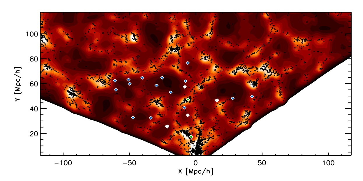
Figure 1: SDSS density map and galaxies in the SDSS galaxy redshift survey region from which we selected the galaxies in the Void Galaxy Survey, in a slice of thickness 4$h^{-1}$Mpc. The DTFE computed galaxy density map, Gaussian smoothed on a scale of $R_{f}=1h^{-1}$Mpc, is represented by the colorscale map. The map runs from dark red, at lowest void densities, to beige, the average cosmic galaxy density. The SDSS galaxies are superimposed as dark dots. The pilot sample void galaxies are represented by white diamonds, while the blue diamonds indicate the position of void galaxies from the full Void Galaxy Survey. The green diamonds are control sample galaxies (see Section 4.5).

A representative DTFE density map in a slice through the SDSS galaxy distribution is shown in Figure 1, with superimposed symbols indicating the original spatial distribution of galaxies and subsequently determined void galaxies.

2.2 Void Galaxy Selection

Upon having obtained the complete list of voids in the SDSS survey volume, and the spectroscopically targeted void galaxies within their realm, we evaluate for each of the galaxies whether it conforms to a set of additional criteria. The galaxy should be

• located in the interior central region of clearly defined voids, if possible near the center, and be as far removed from the boundary of the voids as possible.

• removed from the edge of the SDSS survey volume, as we do not wish to have galaxies in voids which extend past the edge of the SDSS coverage.

• not within $\approx 750$km s^-1 from a foreground or background cluster. This assures that the presence in a void of a galaxy can not be attributed to the Finger of God effect.

• preferably within a redshift $0.01<z<0.02$, allowing sufficient sensitivity and resolution in our observations of the gas structure and kinematics in the galaxies.

Other than the SDSS redshift survey limit of

$$M_{r}=17.77-5\log_{10}\frac{cz}{H_{o}~{}10pc}$$ (4)

there is no selection on luminosity or color of the void galaxies in our sample, the selection is purely dictated by the local geometric structure of the Cosmic Web.

The spectroscopic selection criteria of the SDSS do exclude bright, nearby galaxies and omit some galaxies in particularly crowded fields, however these effects are not relevant to our sample. There is also a poorly constrained surface brightness selection in the SDSS main galaxy sample.

Apart from avoiding the Finger of God effect, note that redshift distortions due to cosmic large scale flows, and as a result of cluster infall, are not affecting our selection. These tend to amplify the density and contrast of filaments, sheets and cluster outskirts in redshift space, while leading to emptier voids: void galaxies detected in redshift space are therefore highly likely to also live in physical voids (cf. Kaiser, 1987; Praton et al., 1997; Shandarin, 2009).

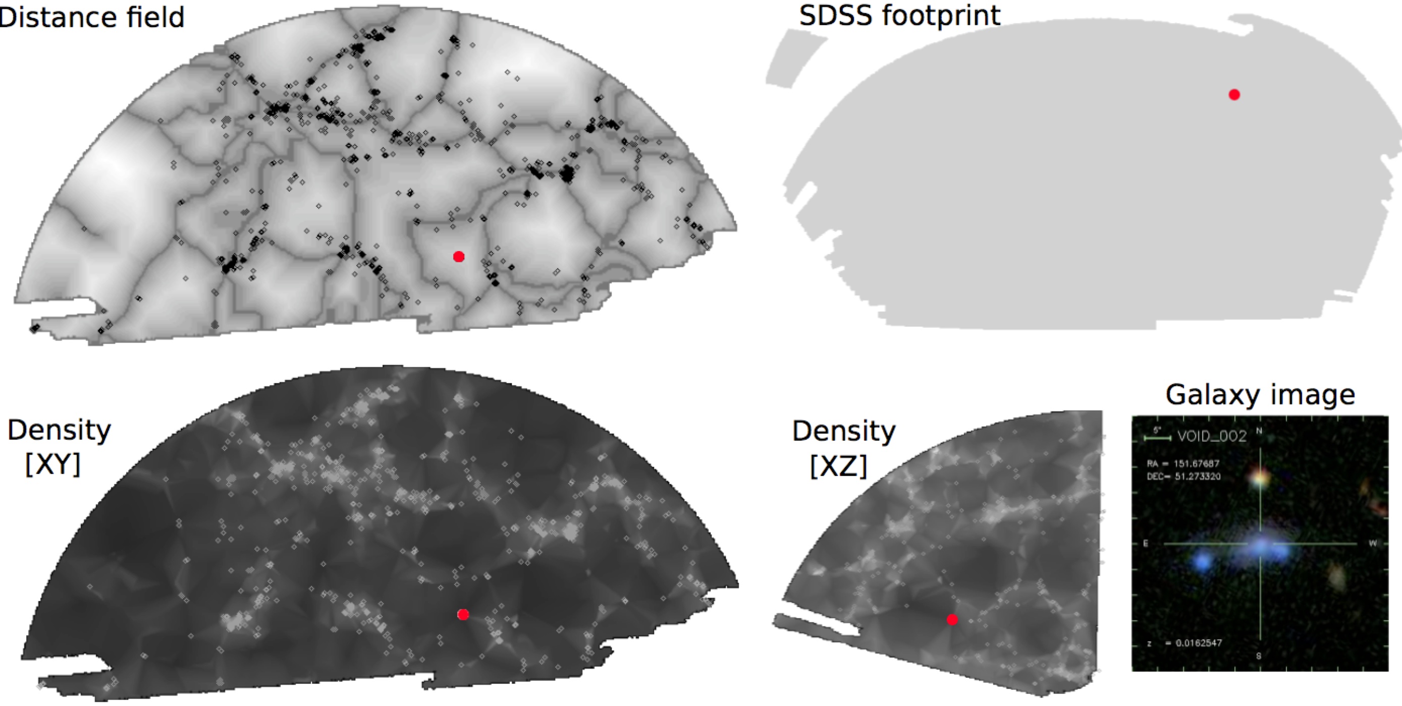
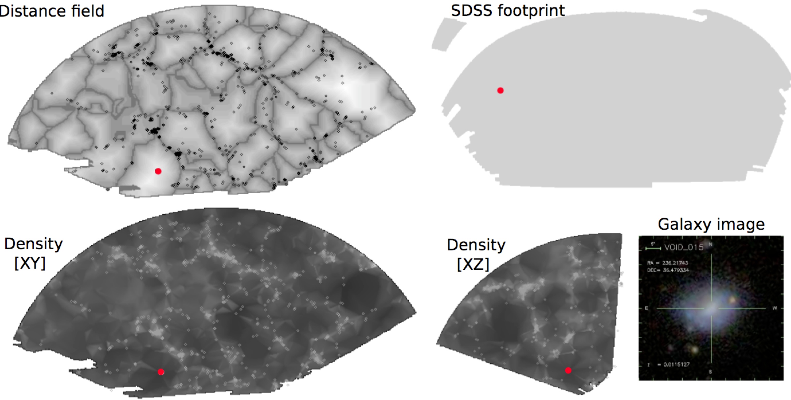
Figure 2: Two examples of selecting our galaxies by geometry from the SDSS using different visualizations of the density field. Top right panel: SDSS DR7 sky map footprint, with the void galaxy indicated by a heavy red dot, to show it is positioned away from the survey edge. Bottom right: galaxy image from SDSS database. Bottom left and center: DTFE density greyscale maps in two mutually perpendicular slices intersecting at the galaxy location. Top left: The SpineWeb/watershed contours of the density field are shown in dark gray on top of the distance field (described in Section 2.2) in gray scale. The locations of the SDSS DR3 galaxies within the thin density field and distance field slices are indicated by the diamond shaped points, while the heavy red dot represents the target galaxy located away from any walls or filaments and deep within the underdensity.

Figure 2 illustrates our selection procedure for two cases. The locations of the void galaxy in the SDSS footprint (heavy dot, top right) are removed from the survey edge and each other. The DTFE density map in two mutually perpendicular slices intersecting at the galaxy location, along the line pointing radially towards the observer (bottom left and center), show their position centrally located in the deepest underdensities. To accentuate this, the images also contain a map of the spinal/watershed contours of the density field overlaid on top of the distance field in order to give an idea of the spatial structure of the surrounding large scale structure (top left). The distance field shows the minimum distance from the void edge, and is maximized at the void center. The locations of the SDSS DR3 galaxies within these thin slices are indicated by the diamond shaped points, while the heavy dot represents the target galaxy. A small galaxy image from the SDSS database (bottom right) shows the optical appearance of our geometrically selected void galaxy.

2.3 Resulting Sample

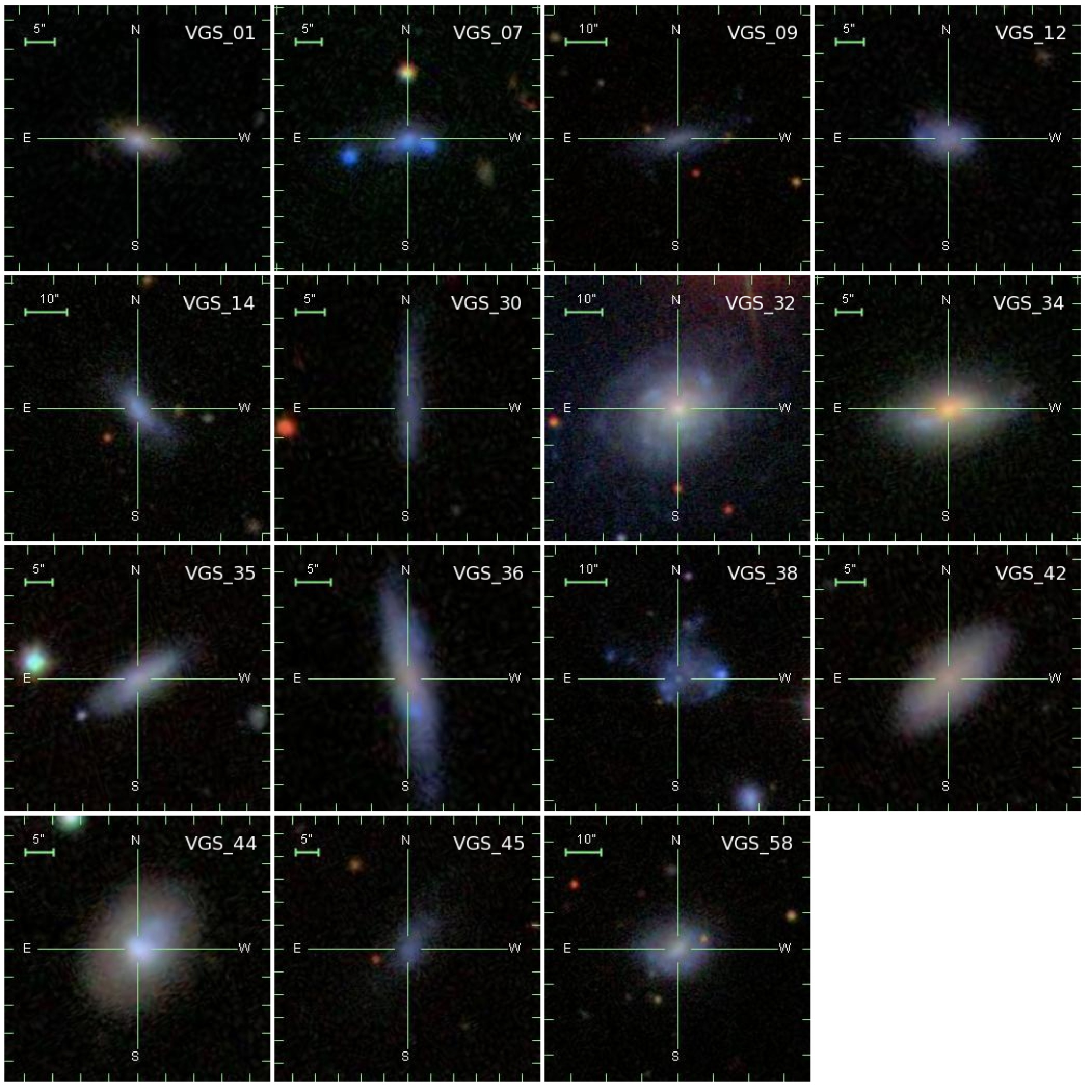
Figure 3: Our sample of void galaxies, scaled to the same physical size. Composite color images are taken from the online SDSS Finding Chart tool.

In Figure 3 we present the SDSS color images of our 15 selected void galaxies, taken from the SDSS online Finding Chart tool (DR7, Abazajian et al. 2009). The images have been scaled to the same physical scale. The parameters for the target galaxies, extracted from the SDSS catalog, are given in Table 1 along with the program and SDSS names. In the remainder, we will mainly use the program name “VGS_$\alpha$”, unless otherwise stated. Likewise, the companion galaxies found in our program will receive a program name “VGS_$\alpha$a”, “VGS_$\alpha$b”, etc., where $\alpha$ is the number for the parent void galaxy.

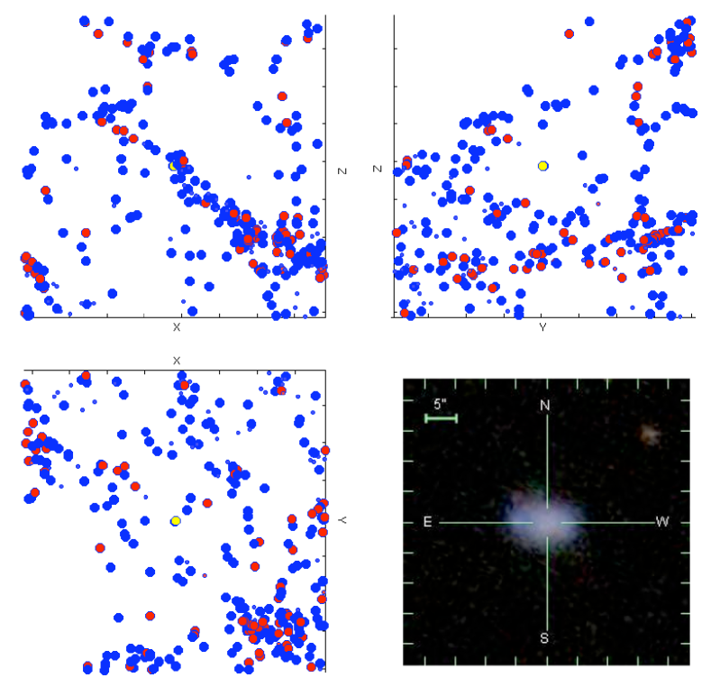
Figure 4: The SDSS galaxy distribution in and around the void in which galaxy VGS_12 of our void galaxy sample is located, seen from three different perspectives. The galaxies are located within a box of size 24 $h^{-1}$ Mpc centered on VGS_12 (in yellow). Bright galaxies have large dots (B $<-16$), fainter ones are depicted by smaller dots. Redder galaxies, with $g-r>0.6$ are indicated by red dots. Bluer galaxies, with $g-r\leq 0.6$, are indicated by blue dots. The SDSS image of the galaxy is shown in the bottom right panel.

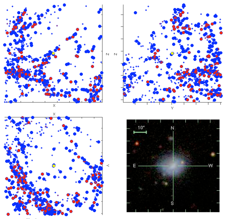
Figure 5: The SDSS galaxy distribution in and around the void in which galaxy VGS_58 of our void galaxy sample is located, seen from three different perspectives. The galaxies are located within a box of size 24 $h^{-1}$ Mpc centered on VGS_58 (in yellow). Bright galaxies have large dots (B $<-16$), fainter ones are depicted by smaller dots. Redder galaxies, with $g-r>0.6$ are indicated by red dots. Bluer galaxies, with $g-r\leq 0.6$, are indicated by blue dots. The SDSS image of the galaxy is shown in the bottom right panel.

To obtain an impression of the true thee-dimensional environment of the selected void galaxies, we have included a set of 3-D galaxy distribution visualizations around void galaxies VGS_12 (Figure 4) and VGS_58 (Figure 5). In a box of size 24 $h^{-1}$ Mpc centered around each of these void galaxies, the structure of the surrounding galaxy distribution is depicted from the three different perspectives. In these panels, bright galaxies have large dots (B $<-16$), while fainter ones are depicted by smaller dots. Redder galaxies, with $g-r>0.6$ are indicated by red dots, and bluer galaxies, with $g-r\leq 0.6$, are indicated by blue dots.

Void 14 lies well within the interior of a huge void, surrounded by filamentary structures. On one side these are embedded within a massive wall-like complex. The geometry of the spatial galaxy distribution around the polar ring galaxy VGS_12 has been discussed at length in Stanonik et al. (2009): the galaxy lies within a tenuous wall in between two voids. This is perhaps most evident in the top left panel, where we see a planar concentration forming the division between a large void (to the top of the box) and a smaller void (to the bottom of the box). A comparison between the spatial distribution of red and blue dots reveals a strong segregation in the low-density regions. In particular the VGS_58 maps illustrate the avoidance by red galaxies of underdense areas. A similar distinction in spatial distribution between faint and bright galaxies is far harder to notice, if at all.

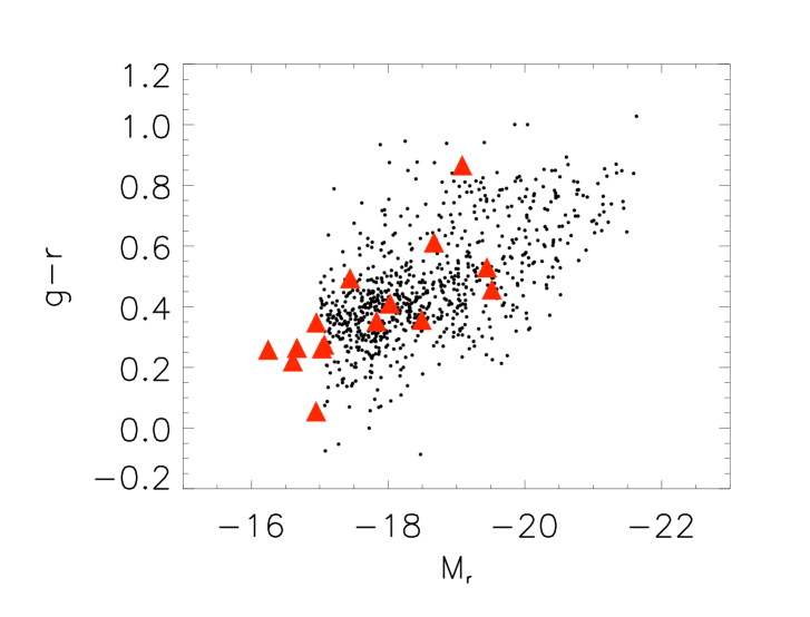
Figure 6: Color-magnitude diagram for our void galaxy sample (triangles), compared with a volume limited ($z<0.02$, M${}_{r}<-16.9$) sample of void galaxies from the SDSS.

The nature of our galaxies can be immediately appreciated from the color-magnitude diagram in Figure 6. For comparison we include a volume-limited sample of galaxies in underdense regions defined by our void-finding algorithm from the SDSS DR7, including all galaxies brighter than $M_{r}=-16.9$ within a redshift range $z<0.02$. Most of our galaxies are in the blue cloud and at the faint end of the galaxy luminosity function, where the bulk of SDSS void galaxies reside. See Section 5 for a detailed discussion of how our void galaxy sample compares with other void galaxies samples.

Table 2 contains parameters for the voids surrounding each target galaxy, taken from our void finding algorithm applied to the SDSS reconstructed density field. For the galaxies that seem to reside in between two voids we have quoted two values, for the two nearest voids.
 
Column (1) lists the program name.
Column (2) lists the (equivalent) void radius $R_{void}$,

$$R_{void}\,\equiv\,\left({\displaystyle 3\,V_{void}\over\displaystyle 4\pi}\right)^{1/3}\,,$$ (5)

where $V_{void}$ is the volume of the void. It corresponds to the radius the void would have if it were spherical.
Column (3) gives $D_{gal,void}$, the distance of the galaxy from the void center.
     Column (4) gives the the ratio of void center distance to void radius,

$$DR\,\equiv\,{\displaystyle D_{gal,void}\over\displaystyle R_{void}}.$$ (6)

Note that nearly all detected voids are elongated, so that galaxies located within the voids’ interior may still have $DR>1$.
Column (5) provides the filtered density contrast of the void,

$$\delta\,\equiv\,{\displaystyle\rho_{void}\over\displaystyle\rho_{u}}\,-1\,\,,$$ (7)

at a filtering scale R${}_{f}=1$h^-1Mpc. Here, $\rho_{u}$ is the mean density, estimated by the average point intensity from the SDSS volume (see Platen 2009).
Column (6) lists the distance to the nearest neighbor.
Column (7) lists the average distance of the six nearest neighbors.
Column (8) gives the void name, taken from Fairall (1998) and Hoyle & Vogeley (2002).

While all targets were ideally chosen for their isolation and central location within the void, our pilot sample selection was limited to the galaxy redshift survey data available with the incomplete DR3. As the catalog has been completed since then some of these targets have proven to be in slightly less centrally located, though still underdense, environments. This, and the fact that most voids have rather elongated shapes, explains why several of the sample galaxies have a distance $R_{void}$ to the void center which is in the order of the (equivalent) void scale $R_{void}$. Galaxies VGS_07, VGS_34, VGS_44, and VGS_58 are the best in terms of location near the center of the void and not near a wall-like configuration.

3 Observations

Our targets were observed 2006-2007 with the Westerbork Synthesis Radio Telescope (WSRT) in Maxi-short configuration. The shortest baselines of 36, 54, 72 and 90 meters optimize surface brightness sensitivity in a single 12 hour observation. Its longest spacing of 2754 meters results in an angular resolution of approximately 20^′′. Observing parameters are detailed in Table 3. We observed using 512 channels per 10 MHz bandwidth, at four simultaneously observed frequencies, each with two polarizations. Along with the observation centered at the target galaxy, three other simultaneous observations were made centered at frequencies 8.3 MHz, -8.3 MHz and -16.6 MHz removed from the target galaxy, resulting in a velocity coverage of nearly 10,000 km s^-1 with each telescope pointing. Target redshifts ranged from 0.012 to 0.022, so channel increments of 19.5312 kHz give a typical velocity resolution of 4.25 km s^-1 using the heliocentric optical velocity definition. After applying Hanning smoothing this is reduced to 8.6 km s^-1. The full width at half maximum of the primary beam is about 36^′, which at a typical redshift of 0.015 is a 700 kpc $\times$ 700 kpc area on the sky.

Each observation consisted of a 12 hour target exposure, calibrated by two 15 min snapshots, one observed before and one observed after, using two of 3C48, 3C286, 3C147 and CTD93. Due to the location’s impressive phase stability, our calibration observations once every 12 hours are sufficient for phase calibration. The absolute flux scale is determined using the flux scale of Baars et al. (1977) in the AIPS task SETJY. At a first channel frequency of 1406.9212 MHz, a corresponding flux of 14.79 Jy, 16.00 Jy, and 22.10 Jy are used for 3C286, 3C48, and 3C147, respectively. For the non-standard calibrator CTD93 we use the 20 cm flux of 4.83 Jy, as listed in the VLA calibrator manual. All calibration is done using standard AIPS procedures.

Continuum emission is subtracted from the UV data by interpolation from the line free channels. Image cubes are created with a CLEAN box around the H i emission that cleans down to 0.5 mJy beam^-1 (1 $\sigma$). Images are created with a robust parameter of 1 (Briggs, 1995) and corrected for the primary beam. Data cubes are then Hanning smoothed to achieve a sensitivity of 0.4 mJy beam^-1. Zeroth and first moment maps are made over a narrow velocity range encompassing the detection, with Hanning and Gaussian smoothing over 25 km s^-1 and 30^′′ and 1.5$\sigma$ clipping. For galaxies removed from the beam center the cutoff value is scaled to correct for the primary beam.

The continuum baseline fit from the line free channels, which is used to determine the continuum subtraction in the UV data, is also used to create a 1.4 GHz continuum image. Images are created with a robust parameter of 1 and CLEANed down to 0.2 mJy beam^-1 (1.5 $\sigma$).

The separation between a void galaxy and the edge of the neighboring velocity range is about 5 MHz once edge channels are excluded, which at the average distance of 70 Mpc corresponds to a cosmological distance of $\sim$15 Mpc. This is large enough to distinguish these neighboring velocity ranges as removed from the target void, which maximally extend to about 15 Mpc in radius (Table 2). For blind H i detections throughout the neighboring velocity range, excluding the target galaxy, data cubes are smoothed to 20 km s^-1 with a 6 kilowavelength taper, producing a 40^′′ beam and 1$\sigma$ sensitivity of 0.25 mJy beam^-1. Zeroth moment maps are made with Hanning and Gaussian smoothing and 5$\sigma$ clipping before correcting for the primary beam to provide a simple blind detection algorithm. We then selected by eye the regions with HI emission that are extended both spatially and in velocity and call this our control sample.

4 Results

In our sample of 15 void galaxies (Table 1 and Figure 7) we have one non-detection, and discovered one previously known and five previously unknown companions (Table 4 and Figure 8). Of the five void galaxies with companions, two are interacting in H i. All H i-detected companions have optical counterparts within the SDSS. Of the nine isolated void galaxies, two exhibit clear irregularities in the kinematics of their gas disks. Target galaxies have a range of H i masses from $3.5\times 10^{8}M_{\odot}$ to $3.8\times 10^{9}M_{\odot}$ and one non-detection with a 3$\sigma$ upper limit of $2.1\times 10^{8}M_{\odot}$, assuming a 150 km s^-1 velocity width. Companion galaxies have masses ranging from $5.0\times 10^{7}M_{\odot}$ to $4.5\times 10^{8}M_{\odot}$. H i properties of the target and companion galaxies are given in Table 5.

4.1 HI Data

H i mass is calculated using the standard formula, $M_{\textrm{H {I}}}=2.356\times 10^{5}\>$d${}^{2}\int$S$\>dv\;M_{\odot}$, where d is the distance in Mpc, S is in Jy and dv is in km s^-1. The integrated flux is taken from the total intensity maps described in Section 3. A rough global profile is constructed by summing the flux in a tight box surrounding the target. The 50% H i line width ($W_{50}$) and 20% H i line width ($W_{20}$) are corrected for instrumental broadening following Verheijen & Sancisi (2001), and broadening due to random motions is neglected. Errors of 15 km s^-1 reflect uncertainties of one channel on either side. Systemic velocities are estimated from tilted ring fits of the velocity field, with typical errors of 5 km s^-1.

Because the majority of the void galaxies are not well enough resolved to reliably fit tilted rings to the kinematics of the gas disk, we measure the radial surface density profile following the iterative deconvolution method described by Lucy (1974) as implemented by Warmels (1988). This technique projects the two dimensional surface brightness map along the disk minor axis to create a one dimensional strip distribution which shows projected surface brightness as a function of position along the disk major axis. Assuming an azimuthally symmetric and circular disk, this strip distribution is then iteratively modeled to reconstruct the radial surface density profile (Figure 9). As discussed by Swaters et al. (2002), this iterative deconvolution method is known to restore too much flux to the disk center, so while the iterative fit was stopped at 10 iterations to prevent this, we may systematically be slightly underestimating our radii and significantly overestimating our central surface densities. Position angles are determined by considering both the $g$-band optical as well as the H i kinematic major axes. The H i radius, R${}_{\textrm{H {I}}}$, is taken as that point where the surface density drops below 1 $M_{\odot}$ pc^-2. Upper limits are listed for those galaxies with an H i extent smaller than the synthesized beam size. Typical uncertainty in the radius is 5^′′, about 1.5 - 2 kpc for our void sample. This is much larger than the typical 0.5^′′ (150 - 200 pc) errors in the optical r₉₀ radius, containing 90% of the Petrosian flux.

As all detected target galaxies exhibit disklike rotation, the inclination corrected circular velocity is used to estimate a dynamical mass, $M_{dyn}$, for the volume interior to R${}_{\textrm{H {I}}}$ as

$$M_{dyn}(r<R)=\frac{W_{50}^{2}R_{\textrm{H {I}}}}{\sin^{2}i~{}G}\;M_{\odot}.$$ (8)

Inclinations, $i$ are calculated from SDSS $r$-band isophotal major and minor axes. Following the assumption that disks be intrinsically oblate and axisymmetric, with a three dimensional axis ratio of q_o = 0.19 (Geha et al., 2006), we use

$$\sin i=\sqrt{\frac{1-(b/a)^{2}}{1-q^{2}_{o}}}.$$ (9)

A choice of q_o = 0.3 changes the resulting inclinations by less than 10%. For targets which have no cataloged $r$-band major and minor axes, we use $u$-band values. The $r$-band and $u$-band inclinations are generally in agreement to within 10%. Due to these uncertainties in the inclination and in the H i radius we expect our dynamical masses to be accurate within roughly a factor of two.

4.2 Radio Continuum Data

Continuum images, with a typical sensitivity of 0.12 mJy beam^-1, are used to calculate at 1.4 GHz star formation rate following Yun et al. (2001), as

$$SFR_{1.4GHz}=\frac{L_{1.4}(ergs~{}s^{-1}~{}Hz^{-1})}{1.7\times 10^{28}}M_{\odot}~{}year^{-1}.$$ (10)

Continuum emission is detected in only four void galaxies, and only two are extended enough (VGS_07 and VGS_32) to rule out confusion with possible active galactic nucleus (AGN) emission, however all radio luminosities are low enough that the net AGN contribution should be small. For those galaxies without emission we calculate a 3$\sigma$ upper limit (Table 6), which we find to be in general agreement with the H$\alpha$ star formation rate (described below).

4.3 Optical Data

To determine the stellar mass of the galaxies from the SDSS optical spectra, each spectrum is pre-corrected for dust extinction due to the Milky Way using the map by Schlegel et al. (1998). Adopting the approach used by various authors (e.g., Gwyn & Hartwick, 2005; Salim et al., 2007), the stellar mass is determined by fitting to the full galaxy spectra (3800–9200 Å  in the observed frame) from the SDSS DR6 (Adelman-McCarthy et al., 2008) the dust-attenuated Bruzual & Charlot (2003) stellar population model spectra, where the dust model of Calzetti et al. (2000) is used to correct for intrinsic dust extinction. The overall model is composed of simple stellar populations with stellar age ranges from 5 Myr to 11 Gyr and stellar metallicity ranges from 0.004 to 0.05. The dust extinction is a free parameter which is determined simultaneously through the best-fit stellar continuum. Using a galaxy sample that is all galaxies included in both the SDSS DR4 and the SDSS DR6 data, the agreement between our dust-free stellar mass estimates and those from the line-indices approach performed upon the SDSS DR4 galaxies (Kauffmann et al., 2003) is on average $\sim$0.25 dex (Yip et al. 2010 in prep.).

As the SDSS spectroscopy samples the light of each galaxy in the central 3^′′-diameter area, an aperture correction is applied in deriving the stellar mass of the whole galaxy. The correction is taken to be the ratio between the flux within the Petrosian radius (which encompasses more than $\sim$90% of a galaxy regardless of the light profile, Strauss et al., 2002) to that within the central 3^′′  diameter of each galaxy, as such $\mbox{m}_{*}^{\mathit{petro}}=\mbox{m}_{*}^{\mathit{fiber}}\,10^{-0.4\,(m^{\mathit{petro}}-m^{\mathit{fiber}})}$, where $\mbox{m}_{*}$ and $m$ denote the stellar mass and the observed frame magnitude of the galaxy, respectively. Stellar masses and H$\alpha$ star formation rates, as determined by the H$\alpha$ luminosity of the optical spectra with an aperture correction applied, are given in Table 6.

Even though we are considering a galaxy population which may be systematically different, our stellar mass estimates are accurate within the tolerances of the method, and are relatively insensitive to the assumed parameters for stellar age and metallicity. Our void galaxy sample shows an agreement of $\sim$0.25 dex between our stellar mass estimates and those in the MPA-JHU DR7 catalog which is based on fits to the photometry through an approach similar to Kauffmann et al. (2003) and Salim et al. (2007). Our choice of the modeled stellar age lower bound, 5 Myr, ensures that the massive stars ($\sim{100}$ $M_{\odot}$) are included in the model. On the choice of the modeled stellar metallicities: the stellar masses are expected to be fairly insensitive to the modeled stellar metallicities, because they are derived from the stellar continuum luminosity, whereas the stellar metallicity of the galaxies affects primarily the absorption line strengths. On the other hand, the stellar mix does determine the amplitude of the underlying stellar absorption in the H$\alpha$ line. The average H$\alpha$ stellar absorption in the SDSS galaxies is ${1.3}$ Å (Hopkins et al., 2003; Miller et al., 2003) determined through an approach which is independent of stellar population model, and is small compared with the average restframe H$\alpha$ emission equivalent width of our galaxies, calculated to be about ${50}$ Å.

4.4 Notes on Individual Void Galaxies

Many of our void galaxies appear morphologically and dynamically quite unexceptional. VGS_09, VGS_14, VGS_36, VGS_42, VGS_45, and VGS_58 all appear to exhibit regular disk-like rotation in their H i contours, and a fairly smooth, disk-like stellar component. At 3$\sigma$ contour levels their H i appears uniform and axisymmetric within resolution limits. However, our small sample does include a number of notable individual galaxies.

VGS_07 has a faint companion which does not appear to be interacting. It exhibits a clumpy, knotty, blue morphology similar to that seen in chain-galaxies forming at high redshift, or like edge-on, low surface-brightness galaxies. It has an enormous 200 Å H$\alpha$ equivalent width, suggesting a high star formation rate per unit stellar mass, and possible starburst. We see fairly regular disk-like kinematics within the gas distribution. It sits near the center of the void and not near a wall-like configuration.

VGS_12 is a polar ring galaxy, and is discussed in detail in Stanonik et al. (2009). It is one of the most massive of our sample, in both its H i ($3.0\pm 0.5\times 10^{9}\;M_{\odot}$) and dynamical ($1.5\times 10^{11}M_{\odot}$) mass, and is substantially more massive in H i than stellar mass ($1.05\times 10^{9}M_{\odot}$). In addition, its H i disk is extremely extended compared to the optical, yet free of stars down to the SDSS surface brightness limits, ruling out most merger scenarios. Simulations can reproduce such gas-rich, star-poor rings through tidal encounters, however at equal mass ratios they destroy the rotational support of the central galaxy, resulting in the formation of an elliptical remnant (Bournaud et al., 2005). The low concentration index, $r_{90}/r_{50}$, of 2.25 implies the central stellar disk is late type (Shen et al., 2003) and thus rotationally supported, suggesting an alternative formation mechanism such as slow accretion of cold gas is necessary (Iodice et al., 2006). In addition, VGS_12 is situated in a thin wall between two voids, and aligned such that this gas would have been accreted out of the voids.

VGS_30 is accompanied by a similar sized H i rich companion. The two are seen to be embedded in a common H i envelope, and due to the thinness of the target galaxy disk, presumably they are interacting for the first time. They are cosmologically situated in a void wall between two large voids.

VGS_32 is particularly close by, and thus significantly better resolved in optical and H i imaging. It displays a quite beautiful flocculent spiral pattern, and a textbook flattened rotation curve. It sits nicely isolated in the middle of a void.

VGS_34 has a very faint, kinematically distinct protuberance in H i. The disturbed optical morphology also suggests that the target is undergoing some sort of interaction, as the bulge appears extremely red while the farther reaches of the disk appear relatively blue and distorted. The H i extention does align with a small, distant H i detected companion. VGS_34 also has a very large rotational velocity. Like VGS_07, it sits near the center of the void and not near a wall-like configuration. Because the SDSS fiber only contains light from the central red bulge, stellar mass and star formation rate parameters derived for this galaxy may not accurately represent the galaxy as a whole.

VGS_35 presents a fairly regular appearance in H i, except in its orientation. We see it exhibiting a strong warp, or perhaps a mis-aligned H i disk as we see in VGS_12. This is complicated by the elongated beam, which is suspiciously aligned with the H i in the disk. Possibly the elongation of the beam is exaggerating a slight warp in the H i disk, as the velocity contours in the center appear aligned with the optical disk, and bend away only in the outer parts. It is located near the transition of a small void into a larger one.

VGS_38 has the most optically disturbed appearance, and it was also the only selected void galaxy to have a known companion, VGS_38a, which is only 12 kpc away on the sky and at nearly overlapping velocity. The surprising discovery of a third galaxy, VGS_38b, aligned with the first two, all three of which are connected by a faint 1$\sigma$ H i bridge, results in a system that stretches nearly 50 kpc across the sky. VGS_38, despite its chaotic appearance, exhibits relatively smooth rotation in the direction perpendicular to the line of galaxies. It is difficult to understand how this system could have undergone a major, disruptive interaction while leaving the gas disk unperturbed. It is located at the edge of its void.

4.5 Control Sample

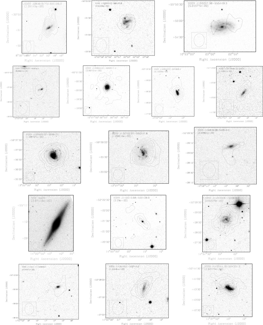
Figure 10: Control sample. Contours in the total intensity maps are at intervals of 2$\sigma$, with the corresponding column density value (in units of $cm^{-2}$) given in the top left corner of each image. Note that low signal to noise results in relatively high 2$\sigma$ column densities of $\sim 2\times 10^{20}cm^{-2}$. Contours for NGC 5422 represent a 1$\sigma$ detection.

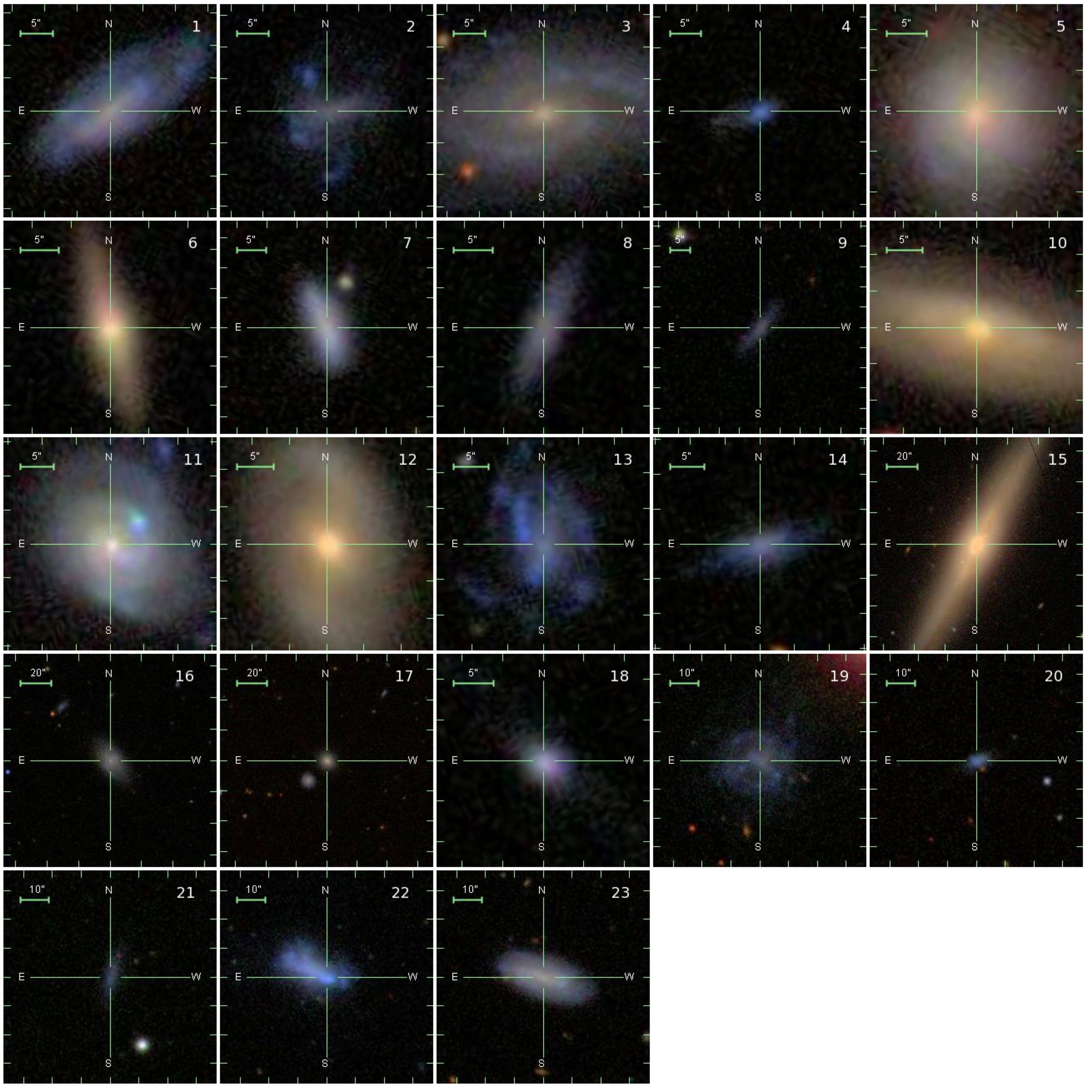
Figure 11: Our control sample galaxies, scaled to the same physical size as the void galaxy sample in Figure 3. Composite color images are taken from the online SDSS Finding Chart tool.

From projection of each observation’s primary beam through the SDSS redshift catalog we find that there are 22 SDSS galaxies in the neighboring velocity ranges of our data set. From our H i blind search for control sample galaxies (described in Section 3), we detect 11 of the known SDSS galaxies and have upper limits for another seven, with mass limit $M_{\textrm{H {I}}}=2.9\times 10^{4}$ d² $M_{\odot}$, d in Mpc and assuming a velocity width of 100 km s^-1. The data on the remaining four galaxies were badly affected by man made interference and could not be used. We also include with this control sample five galaxies detected in H i which are not in the SDSS redshift survey, all with optical counterparts. This brings the control sample to a total of 23 galaxies. We calculate the environmentally filtered density contrast (see Section 2) for each control sample galaxy, and find almost all of them are in average or overdense environments. The $g$-band images with H i contours of all H i detected control galaxies are presented in Figure 10, and color images of all control galaxies are presented in Figure 11.

To ensure confidence in our detections we only consider galaxies within 25^′ of the beam center, which corresponds to a factor of five reduced sensitivity. The combination of larger distances and displacement from the beam center produces fairly low S/N detections, resulting in larger mass uncertainties than for our targeted void galaxies. The lowest H i contour levels for our control sample (Figure 10) correspond to roughly twice the column density as the H i contours for our void galaxies (Figure 7). The H i mass detection of NGC 5422 is actually less than the estimated error, however kinematics and spatial coincidence with the optical galaxy allow us to identify this as a real detection. Parameters for all detected and nondetected control galaxies are listed in Tables 7, 8 and 9.

5 Analysis

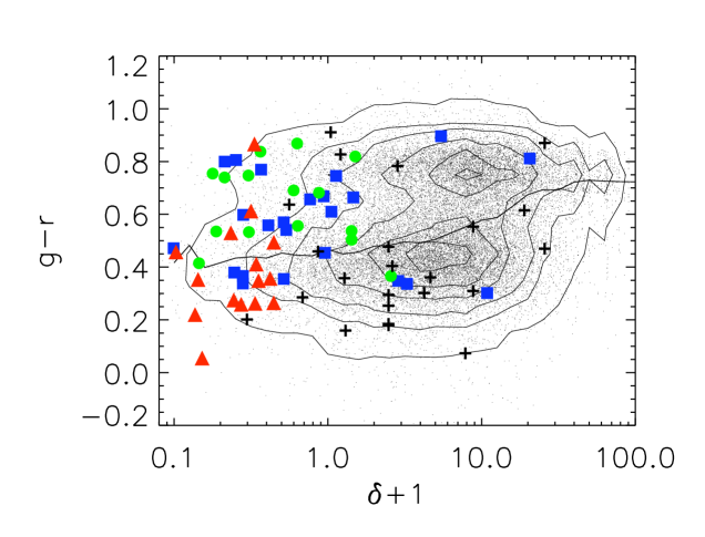
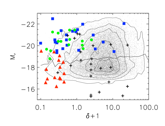
Figure 12: Distribution of $g-r$ colors and $r$-band absolute magnitudes for our void galaxy sample (triangles), our control galaxy sample (crosses), the Boötes void galaxy sample of Szomoru et al. (1996) (squares) and the CfA void galaxy sample of Grogin & Geller (1999) (circles) as a function of density, compared with a volume limited ($z<0.02$, M${}_{r}<-16.9$) sample of SDSS galaxies (points, with contours to guide the eye). The line represents the median of the SDSS sample.

Our void galaxy sample is carefully selected to represent the galaxies populating the deepest underdensities (Figure 4, 5). For comparison we constructed a volume-limited ($z<0.02$, $M_{r}<-16.9$) comparison sample of SDSS galaxies, and use our DTFE procedure to calculate the density field (see Section 2). Eleven of our 15 void galaxies fall within these volume-limited criteria. In Figure 12, we compare the properties of the volume-limited sample as a function of density with our void sample, the IRAS selected Boötes void galaxy sample of Szomoru et al. (1996), and the second Center for Astrophysics redshift survey (CfA2) lowest density void galaxy subsample of Grogin & Geller (1999). Due to the incompleteness of past redshift surveys and brighter magnitude limits, the densities of the Boötes void galaxies and the CfA2 void galaxies have been recalculated based on their inclusion in the SDSS following our method described in Section 2, which results in the identification of many of these galaxies as being in average or even overdense environments. In this respect we emphasize the advantage of using the localized and better defined density values of the DTFE method, defined by the spatial galaxy distribution itself, as opposed to more conventional artificially filtered density values. As a result, our geometric selection criterion manages to probe a galaxy population which is truely representative of the extremely underdense and desolate void interiors, instead of the more conventional techniques probing the galaxies near the void boundaries.

The main photometric and spectroscopic comparison sample of void galaxies against which we measure our pilot sample of geometrically selected void galaxies is that used by Rojas et al. (2004) and Rojas et al. (2005). Their sample of 1010 void galaxies out to z=0.089 was compiled from the first SDSS data release, where they define a void galaxy as having the third nearest neighbor be at a distance greater than 10 Mpc. All other galaxies are placed into a wall galaxy sample. Within these samples they constructed a bright (M${}_{r}\leq-17$) and nearby (d $<$ 103 Mpc) subsample of 76 void galaxies and 1071 wall galaxies. Although our geometric method is very different, ten of our void galaxies satisfy these luminosity and distance criteria.

As has been noted by e.g. Rojas et al. (2004), more luminous galaxies prefer denser environments, and our void galaxy sample is able to probe specifically those low luminosity galaxies which make up the bulk of the void galaxy population that were previously inaccessible. Also apparent in Figure 12 is the dominance of blue galaxies at the deepest underdensities, where we again are more accurately sampling the void galaxy population. For our 10 bright, nearby void galaxies, we find a median $r$-band luminosity of -18.3 $\pm$ 0.3, and median $g-r$ color of 0.46 $\pm$ 0.06, which is in good agreement with the bright, nearby void galaxy sample of Rojas et al. (2004). We also note that our control sample is fairly representative of the range of absolute magnitudes, colors, and densities contained within the SDSS.

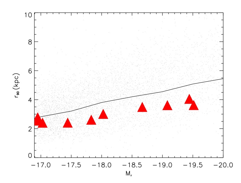
Figure 13: The $r$-band r₉₀ radii of the stellar disk. Our late-type void galaxies (triangles) fall systematically below the median (line) of a volume limited SDSS sample of late-type galaxies (dots).

While we have selected void galaxies with a representative distribution of absolute magnitudes, we find that our void galaxies have stellar disks that are smaller than average. Compared with the volume limited SDSS sample, we find the $r$-band r₉₀ radius of our late type void galaxies is systematically lower than the median for late type galaxies (Figure 13), where galaxies with a concentration index r₉₀/r₅₀ $<$ 2.86 are taken to be late type following Shen et al. (2003).

While our targeted void galaxies are small, they would generally not be classified as dwarf galaxies. All have M${}_{r}<$ -16 and exhibit moderate circular velocities, typically 50-100 km s^-1. All galaxies exhibit signs of rotation in H i, though limiting resolution and lower sensitivity at the disk outskirts means we do not always see a flattening of the rotation curve. $M_{dyn}$ is typically 10⁹ to 10${}^{10}M_{\odot}$. The companion galaxies detected are mostly dwarf galaxies, however our small number statistics for this pilot sample limit us from extending these few detections to draw conclusions on the missing dwarf galaxy population pointed out by Peebles (2001).

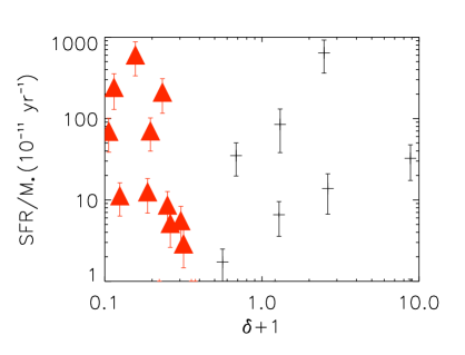
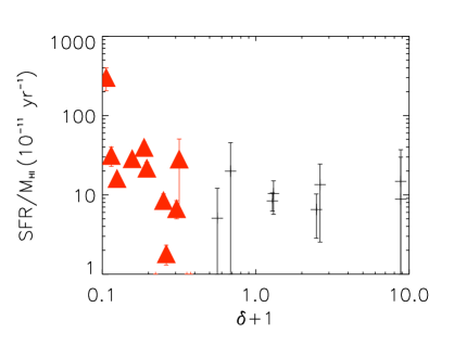
Figure 14: S-SFR (left) and SFR/H i mass (right) as a function of density for our void galaxies (triangles) and our control sample (crosses).

The stellar and star formation properties of our nearby, bright sample measured from the SDSS spectra are in general agreement with the values found for the nearby, bright void galaxy sample of Rojas et al. (2005), and show our pilot sample to be a good representation of the actively star-forming galaxies typically found in voids (Table 10). Even our small sample exhibits the same trend for increased H$\alpha$ equivalent width, star formation rate (SFR) and specific SFR (star formation rate per stellar mass, S-SFR) in low density environments when compared with the wall sample of Rojas et al. (2005). Despite these average increases, we do not see a clear trend of S-SFR with density, but we do see a hint of a trend for increased SFR per H i mass at the lowest densities (Figure 14). The mean S-SFR for our full void sample is $(88\pm 45)\times 10^{-11}$ year^-1 and for our control sample is $(82\pm 63)\times 10^{-11}$ year^-1. The mean SFR per H i mass is $(37\pm 22)\times 10^{-11}$ year^-1 for our void sample and $(11\pm 2)\times 10^{-11}$ year^-1 for our control sample. Our complete sample of 60 void galaxies will be more suitable for the identification of possible trends with density.

Because our control sample for this pilot study is not very large, we have drawn from the literature two additional comparison samples with which to compare H i properties. The first is a sample of 113 late-type dwarf and irregular galaxies from the WHISP project (Westerbork observations of neutral Hydrogen in Irregular and SPiral galaxies, van der Hulst et al. 2001) observed with the WSRT, selected to have Hubble type later than Sd or magnitude fainter than $M_{B}=-17$ (Swaters et al., 2002, S02). These galaxies were not selected in any way for environment, and in general their cosmological environments are unknown. In an attempt to control for environment, we also compare with the H i imaging survey of 43 Ursa Major galaxies brighter than -16.8 and more inclined than 45^∘ with the WSRT (Verheijen & Sancisi, 2001, VS01). Because of their shared membership in the Ursa Minor poor cluster, we assume some uniformity of environment within this comparison sample.

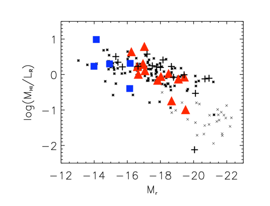
Figure 15: H i mass to light ratio for our targeted void galaxies (triangles), companion galaxies (squares), and our control galaxies (crosses). For additional comparison, late-type disk galaxies from Swaters et al. (2002) (stars) and Ursa Major galaxies from Verheijen & Sancisi (2001) (X’s) are included.

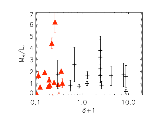
Figure 16: H i mass to light ratio as a function of density for our void galaxies (triangles) and our control sample (crosses).

While optically our sample is blue with higher star formation rates than galaxies in average density environments, the H i content appears to be more typical. As in Geha et al. (2006), we find that the smallest galaxies are the most gas-rich. Figure 15 shows that the ratio of $M_{\textrm{H {I}}}/L_{r}$ increases with decreasing luminosity similar to S02 and VS01. This trend seems to persist over a wide range of luminosities and environments. Huchtmeier et al. (1997) measured that $M_{\textrm{H {I}}}/L_{B}$ increases with decreasing density. We do not see such a trend with density within our small sample of void galaxies (Figure 16), nor do we see a significant difference between our void sample and control sample, or compared to the higher density comparison samples of S02 or VS01 (Figure 15).

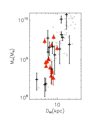
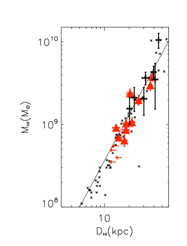
Figure 17: H i mass versus optical diameter on the left, and versus H i diameter on the right. Our target galaxies (triangles) and control sample (crosses) are compared with the sample of late-type galaxies by Swaters et al. (2002) at right (stars) and a cross-match of ALFALFA galaxies (Giovanelli et al., 2007) with the SDSS catalog at left (diamonds). Overplotted on the right is the fit from Verheijen & Sancisi (2001) for their sample of Ursa Major galaxies. Red arrows mark the upper limit on the diameter for those void systems which are poorly resolved in H i.

Our void galaxies follow the tight relation between H i mass and H i diameter demonstrated by S02 and VS01 (Figure 17, right). The agreement of our underdense sample with both comparison samples shows that the mean H i surface density is quite robust, regardless of environment. Galaxy samples also show a correlation between H i mass and optical diameter (e.g. Verheijen & Sancisi (2001)). The range of optical diameters of our void galaxies is too small to look for a trend, but the measured values seem reasonable (Figure 17, left). Our control sample does appear to lie on the correlation. We also note that while the resolution is not optimal, our H i disks typically appear roughly exponential in shape at their outer extent (Figure 9), as was found by S02 for their late type disk galaxies.

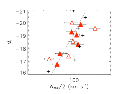
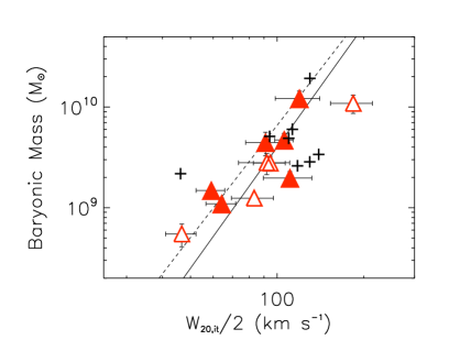
Figure 18: Void galaxies following the I-band (left) and baryonic (right) Tully-Fisher relationship, where the filled symbols are galaxies for which we observe a flattened rotation curve and the open symbols are systems where the rotational velocity continues to rise at the furthest radii. Crosses indicate our control sample galaxies. The dashed lines were taken from Geha et al. (2006) which were fit to over three orders of magnitude mass range. The solid line shows the fit taken from McGaugh et al. (2000).

Hoeft et al. (2006) predict the effects of UV background ionization will suppress star formation and lead to a reduced baryon fraction in small, $M_{tot}\sim 10^{9}M_{\odot}$ halos. Our halos are just on the verge of this boundary, with $M_{dyn}>2\times 10^{9}M_{\odot}$, however we see no deviation from the baryonic Tully-Fisher relationship (Figure 18). W₂₀ values have been corrected for turbulent velocity broadening and inclination angle. Error bars reflect a 10% uncertainty in inclination. Baryonic masses have been calculated from the sum of the stellar mass and 1.4 times the H i mass to estimate the total gas component from our H i measurement. In some of our systems (open triangles) we do not observe a flattening of the rotation curve due to poor resolution or truncated H i disks. As expected, better determined systems (filled triangles) show a tighter correlation and are more consistent in their scatter about the Tully-Fisher relationship, as derived in environmentally insensitive samples (McGaugh et al., 2000; Geha et al., 2006).

6 Speculation

With such a small sample, it is difficult to discuss the statistical properties of our void galaxy sample. It is tempting, instead, to consider the situation of individual galaxies in our sample and the way they might illustrate the larger picture of galaxy evolution in voids which we are interested in investigating.

In some respects we expect to find galaxy evolution progressing within voids somewhat independent of their large scale environment. Simulations show that halos in underdense regions have assembled at later times (Gao et al., 2005), so we would expect that the galaxies we find there to simply be in a slightly earlier stage of their development. This is reflected in the increased number of blue, star forming galaxies found in voids (Rojas et al., 2004, 2005). However the formation of red elliptical galaxies by mergers is not excluded, and in fact the galaxies in the very deepest underdensities cluster more strongly than those in more moderately underdense regions, though less strongly than in average density regions (Abbas & Sheth, 2007). This is similar to the conclusions of Szomoru et al. (1996), who found a similar number of H i companions for void and cluster galaxies. The clustering of dwarf companions appears somewhat consistent, regardless of environment (Weinberg et al., 1991). Our sample probes to lower H i limits than Szomoru et al. (1996), though they covered a much larger volume, and already we find a third of our void galaxies have previously unidentified companions, two of which share a common H i envelope with the targeted void galaxy.

We may expect environment will play some role. Cold mode accretion dominates in low mass halos and at earlier times (Kereš et al., 2009), so we expect to see evidence of this ongoing slow accretion, though it may be difficult to distinguish from the effects of minor mergers. As void galaxies are statistically bluer at fixed luminosity than galaxies at higher densities (Park et al., 2007; von Benda-Beckmann & Müller, 2008), perhaps this is evidence of different mechanisms of gas accretion at play. VGS_12, our void galaxy with a polar disk of H i gas, might provide direct evidence that these processes do occur within voids, as it is difficult to amass such a substantial amount of H i without disrupting the rotational support of the central stellar disk (Bournaud et al., 2005; Stanonik et al., 2009). We also note that the properties which do not seem to be sensitive to the low density environment ($M_{\textrm{H {I}}}/L_{r}$, the ratio of H i mass to H i diameter, the Tully-Fisher relation) are more indicative of the internal effects within the galaxies. The SFR, which we find is tentatively higher in voids, is instead indicative of an external effect, such as higher gas inflow.

Additional evidence of environmental effects should be evident. Hierarchical merging through the expansion of voids and thinning of void walls results in the formation of substructure within voids. Filaments in dark matter which are quite distinct in simulations are tenuously traced by dark matter halos, but depending on the halo occupation distribution may not be apparent in the galaxy distribution, particularly when limited to the distribution of bright galaxies. These alignments may be more apparent in H i as with VGS_38, where the linear alignment of all three galaxies, including the H i bridge between them, may already be sufficient to identify a filament within the void that is not apparent in the SDSS redshift survey.

Filaments which are too low density to be traced by galaxies may still be traced by low column density H i or warm ionized gas (McLin et al., 2002; Manning, 2002; Stocke et al., 2007). The intervening regions between the aligned components we detect near our void galaxies are ideal locations to use background quasars as probes and search for absorption due to underlying filamentary structure.

7 Conclusion

We have completed a pilot study imaging in H i 15 void galaxies selected from the SDSS and located in d $<$ 100 Mpc voids. Galaxies were selected purely by their environment to be located in areas less than half the cosmic density. We detected 14 of our target galaxies with masses from $3.5\times 10^{8}$ to $3.8\times 10^{9}M_{\odot}$, and had one nondetection with a 3$\sigma$ upper limit of $2.1\times 10^{8}M_{\odot}$. In addition we detected six companion galaxies in H i, two of which appear to be interacting with the targeted void galaxy.

We also constructed a control sample from the SDSS redshift survey galaxies and H i detected galaxies in the $\sim$10,000 km s^-1 velocity range simultaneously imaged by the WSRT behind and in front of the target galaxy with each pointing. Of 18 detectable SDSS cataloged galaxies contained within the volume, we detected 11 in H i with masses $6.0\times 10^{7}M_{\odot}$ to $1.4\times 10^{10}M_{\odot}$. In addition, we include five galaxies detected in H i which were not contained in the SDSS redshift catalog. Because of their location within the SDSS footprint we were able to environmentally locate these systems as almost all being in regions at or above the cosmic mean. Due to the small size of this control sample, when comparing specific H i properties of our void galaxies we also looked to comparison samples of well studied galaxies taken from the literature with similar size and luminosity constraints, though their environments are not known.

Provisionally, we find that our void galaxies have small optical stellar disks, typical H i masses for their luminosity, and generally follow the Tully-Fisher relation. Consistent with previous surveys, they have increased rates of star formation, with the suggestion of a trend for increased star formation at lowest density. While this pilot sample is too small for any statistical findings, we did discover many of our targets to be individually interesting dynamically and kinematically in their H i distributions. In particular, one shows possible evidence of ongoing cold mode accretion.

Ultimately, we aim to compile a sample of $\sim$60 void galaxies which will comprise a new Void Galaxy Survey (VGS). This sample size will be comparable to the H i sample of 24 void galaxies and 18 H i detected companion galaxies in Boötes by Szomoru et al. (1996), but more representative of the faint void galaxy population in a more distributed collection of voids. Our sample will also provide a good compliment to the sample of 76 SDSS void galaxies examined photometrically and spectroscopically by Rojas et al. (2004) in similarly nearby voids, and will be ideal for a careful investigation of the questions surrounding how void galaxies get their gas, form substructures and generally populate the most underdense regions of the universe.

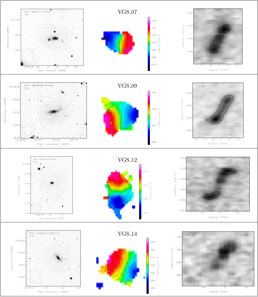
Figure 7:

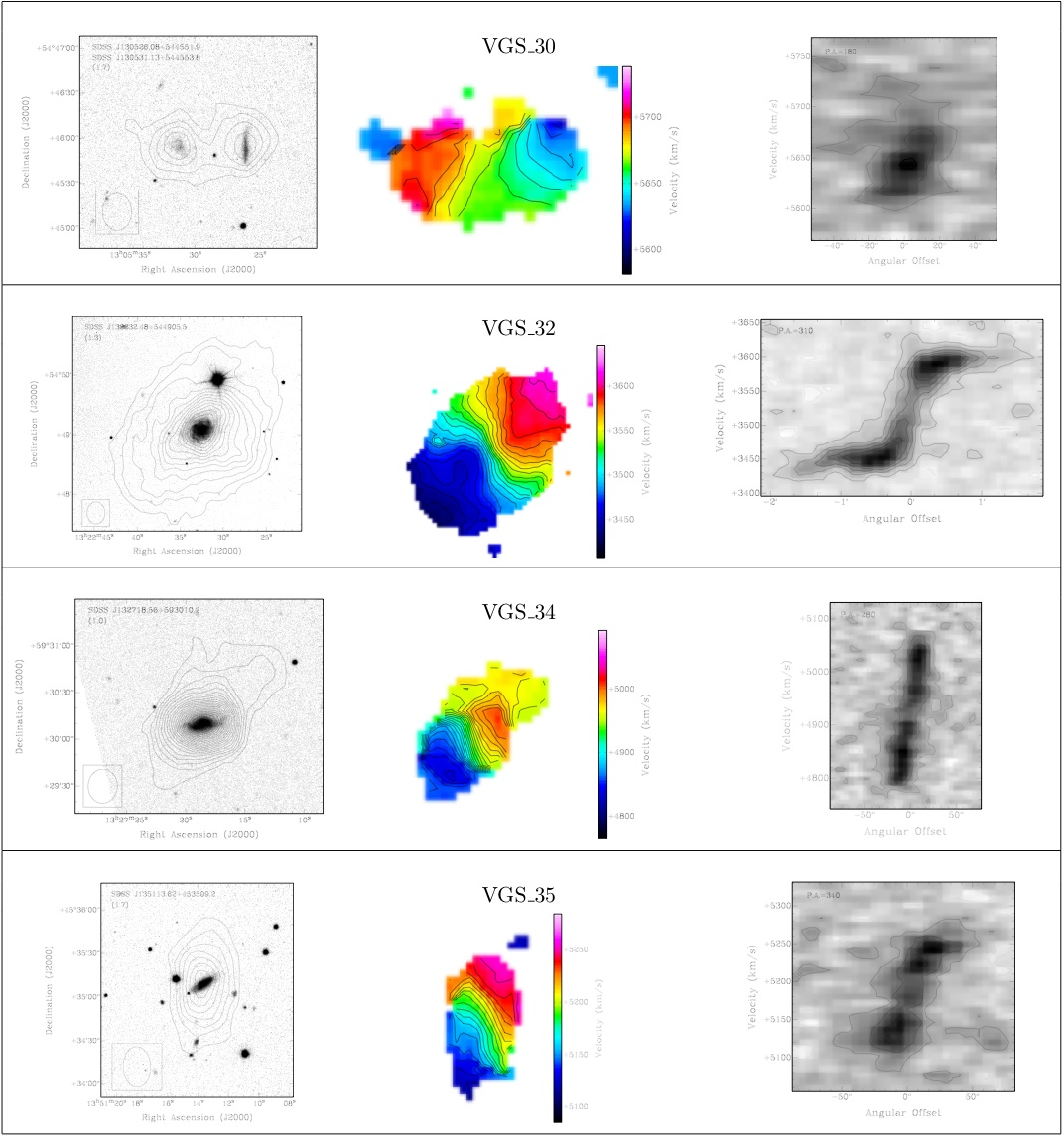
Figure 7:

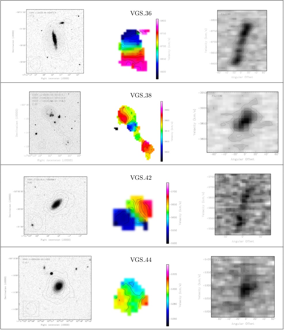
Figure 7:

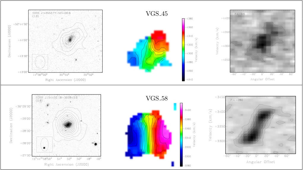
Figure 7: Targeted void galaxies. Contours in the total intensity maps (left) are at $5\times 10^{19}cm^{-2}$ plus increments of $10^{20}cm^{-2}$. Confidence level ($\sigma$) of the lowest contour is given in the top left corner of each image. Lines in the velocity field images (center) indicate increments of 8 km s^-1. Position-Velocity diagrams (right) are along the kinematic major axis, contours are at increments of -1.5 (grey), 1.5 (black) + increments of 3$\sigma$ .

Figure 8: Companions. Note that VGS_30a, VGS_38a and VGS_38b are shown in Figure 7 along with the targeted void galaxy. Contours in the total intensity maps are at $5\times 10^{19}cm^{-2}$ plus increments of $10^{20}cm^{-2}$. Confidence level ($\sigma$) of the lowest contour is given in the top left corner of each image.

Figure 9: Radial surface density profiles for the east (open circles) and west (filled circles) sides of each disk, with the average overdrawn.

Table 1: Parameters of selected void galaxies taken from the SDSS catalog

Name	SDSS ID	ra	dec	$z$	$g$	$r$	$g-r$	Mr
		(J2000.0)	(J2000.0)
VGS_01	SDSS J083707.48+323340.8	08 37 07.5	+32 33 41	0.018531	17.67	17.17	0.49	-17.4
VGS_07	SDSS J100642.44+511623.9	10 06 42.5	+51 16 24	0.016261	17.36	17.30	0.06	-16.9
VGS_09	SDSS J102250.68+561932.1	10 22 50.7	+56 19 32	0.012995	17.78	17.52	0.26	-16.2
VGS_12	SDSS J102819.23+623502.6	10 28 19.2	+62 35 03	0.017804	17.67	17.41	0.26	-17.0
VGS_14	SDSS J103506.46+550847.5	10 35 06.5	+55 08 48	0.013154	16.99	16.72	0.28	-17.1
VGS_30	SDSS J130526.08+544551.9	13 05 26.1	+54 45 52	0.019435	18.27	18.05	0.22	-16.6
VGS_32	SDSS J132232.48+544905.5	13 22 32.5	+54 49 06	0.011835	14.70	14.17	0.53	-19.4
VGS_34	SDSS J132718.56+593010.2	13 27 18.6	+59 30 10	0.016539	16.09	15.22	0.87	-19.1
VGS_35	SDSS J135113.62+453509.2	13 51 13.6	+45 35 09	0.017299	16.77	16.36	0.41	-18.0
VGS_36	SDSS J135535.46+593041.3	13 55 35.5	+59 30 41	0.022398	16.81	16.46	0.36	-18.5
VGS_38	SDSS J140034.49+551515.1	14 00 34.5	+55 15 15	0.013820	17.30	16.95	0.35	-16.9
VGS_42	SDSS J142416.41+523208.3	14 24 16.4	+52 32 08	0.018762	16.49	15.88	0.61	-18.7
VGS_44	SDSS J143052.33+551440.0	14 30 52.3	+55 14 40	0.017656	15.38	14.92	0.46	-19.5
VGS_45	SDSS J143553.77+524400.6	14 35 53.8	+52 44 01	0.014553	17.60	17.33	0.26	-16.7
VGS_58	SDSS J154452.18+362845.6	15 44 52.2	+36 28 46	0.011522	16.05	15.70	0.35	-17.8

Note. — Units of right ascension are hours, minutes, and seconds, and units of declination are degrees, arcminutes, and arcseconds. $z$ is the spectroscopic redshift. $g$ and $r$ list the apparent model magnitudes available in the SDSS DR7 catalog. Absolute magnitudes have been corrected for galactic extinction.

Table 2: Parameters of the voids surrounding the target void galaxies.

Name	Rvoid	Dgal,void	DR	$\delta$	Nearest	Nearest	Void Name
	(Mpc)	(Mpc)			nbr	nbr6
(1)	(2)	(3)	(4)	(5)	(6)	(7)	(8)
VGS_01	16.72	18.48	1.11	-0.68	1.92	2.77	UrsaMajor
VGS_07	16.72	13.39	0.80	-0.82	3.97	4.67	UrsaMajor
VGS_09	16.50	19.77	1.20	-0.67	1.52(4)	4.09	Leo(Top)
VGS_12	18.64/16.72	17.22/17.68	0.92/1.06	-0.78	3.51	4.01	UrsaMinorII/UrsaMajor
VGS_14	16.50	18.37	1.11	-0.68	1.52(2)	4.18	Leo(Top)
VGS_30	16.25	12.69	0.78	-0.85	3.31	5.16	UrsaMinorII
VGS_32	18.64	17.26	0.93	-0.74	3.69	4.65	UrsaMinorI
VGS_34	18.64	9.65	0.52	-0.66	3.39	4.19	UrsaMinorI
VGS_35	16.25	12.71	0.78	-0.57	2.82	4.07	UrsaMinorII
VGS_36	16.25/18.64	15.66/22.03	0.96/1.18	-0.74	2.86	3.67	UrsaMinorII(Top)/UrsaMinorI
VGS_38	18.64	14.98	0.80	-0.58	1.61	3.50	UrsaMinorI
VGS_42	18.64/16.25	19.25/12.79	1.03/0.79	-0.66	1.87	3.80	UrsaMinorI/UrsaMinorII
VGS_44	18.64	15.70	0.52	-0.83	2.99	4.13	UrsaMinorI
VGS_45	18.64	16.50	0.88	-0.38	3.10	3.44	UrsaMinorI
VGS_58	14.57	12.59	0.86	-0.88	0.34	5.26	CoronaBorealisII

Note. —  Listed are: name of the target void galaxy (1), (equivalent) void radius $R_{void}$ (2), the distance $D_{gal,void}$ of the galaxy from the void center (3), ratio of void center distance to void radius (4), the filtered density contrast $\delta$ at R${}_{f}=1$h^-1Mpc (5), the distance to the nearest neighbor (6), the average distance of the six nearest neighbors (7) and the void name taken from Fairall (1998) and Hoyle & Vogeley (2002) (8). See Section 2.3 for further specification.

Table 3: Parameters of the WSRT observations

Configuration	Maxi-short
Date	2006,2007
No. telescopes	13
Exposure time	12 h
Total bandwidth	40 MHz
No. channels	512
Shortest spacing	36 m
Longest spacing	2754 m
FWHM primary beam	36′
Synthesized beam	19${}^{\prime\prime}\times$ 19′′/sin($\delta$)
rms	0.4 mJy Beam-1
velocity resolution	8.6 km s-1

Table 4: Companion galaxies parameters taken from the SDSS catalog

name	SDSS ID	ra	dec	$g$	$r$	$g-r$	Mr	$\Delta\theta$	$\Delta$d	$\Delta$ v
		(J2000.0)	(J2000.0)					(′)	(kpc)	(km s-1)
VGS_07a	SDSS J100519.69+511038.3	10 05 19.7	+51 10 38	20.15	20.12	0.03	-14.1	14.2	288	-21
VGS_09a	SDSS J102241.41+561208.5	10 22 41.4	+56 12 09	22.29	22.26	0.02	-11.4	7.5	121	-85
VGS_30a	SDSS J130531.13+544553.8	13 05 31.1	+54 45 54	18.67	18.39	0.29	-16.2	0.7	17	-74
VGS_34a	SDSS J132640.92+593202.5	13 26 40.9	+59 32 03	20.41	20.31	0.10	-14.0	5.1	104	42
VGS_38a	SDSS J140032.44+551445.9	14 00 32.4	+55 14 46	17.74	17.59	0.15	-16.1	0.6	9	-21
VGS_38b	SDSS J140025.68+551318.5	14 00 25.7	+55 13 19	19.02	18.82	0.20	-14.9	2.3	37	10

Note. — Units of right ascension are hours, minutes, and seconds, and units of declination are degrees, arcminutes, and arcseconds. $g$ and $r$ list the apparent model magnitudes as measured by the SDSS DR7. Absolute magnitudes have been corrected for galactic extinction. $\Delta\theta$, $\Delta$d and $\Delta$v list the displacement from the beam center, projected sky separation, and velocity separation, respectively, between the target and companion galaxy.

Table 5: H i properties of targeted void galaxies and companions

Name	$M_{\textrm{H {I}}}$	$V_{sys}$	D	r90	r${}_{\textrm{H {I}}}$	$W_{50}$	$W_{20}$	i	$M_{dyn}$	$M_{\textrm{H {I}}}/L_{r}$
	($10^{8}M_{\odot}$)	(km s-1)	(Mpc)	(kpc)	(kpc)	(km s-1)	(km s-1)	(∘)	($10^{10}M_{\odot}$)
VGS_01	$<$ 2.1	-	-	2.4	-	-	-	60	-	-
VGS_07	8.6 $\pm$ 0.8	4901	70	2.6	9.2	119	144	50	1.28	1.9
VGS_07a	3.23 $\pm$ 0.65	4880	69	3.5	-	41	49	-	-	9.7
VGS_09	10.3 $\pm$ 1.0	3881	55	3.1	9.1	110	126	68	0.74	4.4
VGS_09a	0.57 $\pm$ 0.14	3796	54	1.5	-	41	49	-	-	20.2
VGS_12	29.9 $\pm$ 4.2	5316	76	2.4	18.0	154	179	29	10.55	6.2
VGS_14	6.4 $\pm$ 1.0	3933	56	3.3	8.7	110	134	67	0.72	1.3
VGS_30	5.5 $\pm$ 1.0	5666	81	3.7	$<$ 7.5	50	93	77	$<$ 0.12	1.7
VGS_30a	4.52 $\pm$ 0.79	5592	79	2.1	-	24	41	-	-	2.1
VGS_32	38.0 $\pm$ 4.5	3522	50	4.1	19.0	171	187	46	6.29	0.9
VGS_34	23.9 $\pm$ 2.9	4917	70	3.6	10.2	231	299	50	5.34	0.7
VGS_34a	0.50 $\pm$ 0.16	4959	70	1.1	-	33	58	-	-	1.7
VGS_35	10.7 $\pm$ 1.3	5191	74	3.0	10.8	145	187	65	1.61	0.9
VGS_36	19.8 $\pm$ 2.7	6684	95	5.0	13.0	190	224	79	2.82	1.1
VGS_38	9.1 $\pm$ 0.7	3853	55	2.8	6.9	50	92	39	0.26	2.0
VGS_38a	0.86 $\pm$ 0.14	3832	54	1.3	-	67	75	-	-	0.4
VGS_38b	1.39 $\pm$ 0.22	3863	55	1.4	-	41	66	-	-	2.0
VGS_42	4.0 $\pm$ 1.5	5601	80	3.5	$<$ 8.1	128	171	58	$<$ 1.08	0.2
VGS_44	4.9 $\pm$ 1.1	5295	76	3.6	$<$ 7.0	76	110	31	$<$ 0.90	0.1
VGS_45	3.5 $\pm$ 1.3	4316	62	4.0	$<$ 6.9	68	102	66	$<$ 0.22	1.0
VGS_58	7.0 $\pm$ 0.6	3351	48	2.6	7.4	143	151	38	2.39	0.7

Note. — Non-detections list the 3$\sigma$ upper limit on the H i mass. $V_{sys}$ is the systemic H i velocity, using the optical definition. D is the distance to the target galaxy. r₉₀ and r${}_{\textrm{H {I}}}$ list the optical and H i radius, respectively. When possible, poorly resolved systems list the upper limit for r${}_{\textrm{H {I}}}$ and $M_{dyn}$. $W_{50}$ and $W_{20}$ are the 50% and 20% H i line widths, respectively, corrected for instrumental broadening. The inclination, $i$, is calculated such that 90^∘ is edge-on.

Table 6: Stellar and star formation parameters for void galaxies

Name	$M_{*}$	SFRHα	SFR1.4GHz	EW(H$\alpha$)	SFR${}_{H\alpha}/M_{*}$	SFRHα/$M_{\textrm{H {I}}}$
	($10^{8}M_{\odot}$)	($M_{\odot}$ yr-1)	($M_{\odot}$ yr-1)	(Å)	($10^{-11}$ yr-1)	($10^{-11}$ yr-1)
VGS_01	6.8	1.43	$<$ 0.16	55.3	211.5	-
VGS_07	0.4	0.25	0.20	202.9	604.4	28.6
VGS_09	0.4	0.00	$<$ 0.08	16.7	0.0	0.0
VGS_12	10.5	0.05	$<$ 0.15	22.4	5.2	1.8
VGS_14	2.0	0.14	$<$ 0.08	53.4	70.7	21.7
VGS_30	0.7	0.17	$<$ 0.17	11.3	241.8	31.5
VGS_32	68.6	-	0.57	15.1	0.0	0.0
VGS_34	75.4	0.95	2.97	32.2	12.6	39.7
VGS_35	12.8	0.07	$<$ 0.14	19.7	5.6	6.7
VGS_36	19.4	0.17	$<$ 0.23	17.0	8.7	8.5
VGS_38	0.5	0.00	$<$ 0.08	-0.3	0.0	0.0
VGS_42	38.9	0.11	$<$ 0.16	9.5	2.9	28.3
VGS_44	21.1	1.47	0.95	85.9	69.8	302.4
VGS_45	0.6	0.00	$<$ 0.10	11.4	0.0	0.0
VGS_58	10.0	0.11	$<$ 0.06	10.9	11.3	16.1

Note. — Targets not detected in the 1.4 GHz continuum list the 3$\sigma$ upper limit on the SFR_1.4GHz.

Table 7: Control sample galaxy parameters taken from the SDSS catalog

#	SDSS ID	ra	dec	$z$	$g$	$r$	$g-r$	Mr	$\delta$	$\Delta\theta$
		(J2000.0)	(J2000.0)							(′)
1	SDSS J083649.77+325109.3	08 36 49.8	+32 51 09	0.025672	16.26	15.90	0.36	-19.4	0.28	17.9
2	SDSS J102002.03+562423.8	10 20 02.0	+56 24 24	0.024881	17.53	17.22	0.31	-18.0	7.81	23.8
3	SDSS J102257.38+555449.3	10 22 57.4	+55 54 50	0.025082	15.63	15.08	0.55	-20.1	7.81	24.7
4	SDSS J102316.27+562656.2	10 23 16.3	+56 26 56	-	18.57	18.50	0.07	-16.6	6.84	8.2
5	SDSS J102653.21+622011.4	10 26 53.2	+62 20 12	0.031975	15.41	14.78	0.64	-20.9	-0.44	17.9
6	SDSS J102823.88+623706.6	10 28 23.9	+62 37 07	0.030462	16.39	15.60	0.78	-20.0	1.84	2.2
7	SDSS J102942.07+624826.2	10 29 42.1	+62 48 27	0.023326	16.64	16.24	0.40	-18.8	1.63	16.5
8	SDSS J103105.76+623531.5	10 31 05.8	+62 35 32	0.030938	18.09	17.73	0.36	-17.9	3.65	19.2
9	SDSS J130418.89+544209.9	13 04 18.9	+54 42 10	-	18.81	18.50	0.30	-15.7	3.23	10.4
10	SDSS J132433.97+592018.6	13 24 34.0	+59 20 19	0.028574	15.29	14.38	0.91	-21.1	0.04	23.1
11	SDSS J132523.37+593643.1	13 25 23.4	+59 36 43	0.026625	15.10	14.65	0.46	-20.7	-0.13	16.0
12	SDSS J132630.72+594313.7	13 26 30.7	+59 43 14	0.029162	15.30	14.48	0.83	-21.1	0.21	14.4
13	SDSS J132722.97+592537.8	13 27 23.0	+59 25 38	0.028064	16.96	16.80	0.16	-18.7	0.31	4.6
14	SDSS J135839.08+552910.3	13 58 39.1	+55 29 10	0.027418	18.06	17.86	0.20	-17.5	-0.70	21.5
15	NGC 5422	14 00 42.0	+55 09 52	0.006071	12.93	12.06	0.87	-20.1	24.71	5.5
16	SDSS J140058.24+553405.1	14 00 58.2	+55 34 05	0.006174	16.37	15.90	0.47	-16.2	24.71	19.1
17	SDSS J140101.95+545555.2	14 01 02.0	+54 55 55	0.005950	17.31	16.69	0.61	-15.4	17.97	19.7
18	SDSS J142515.68+522128.9	14 25 15.7	+52 21 29	0.031980	17.84	17.56	0.29	-18.2	-0.32	14.0
19	SDSS J143422.81+522839.0	14 34 22.8	+52 28 39	-	16.51	16.26	0.25	-17.2	1.48	20.6
20	SDSS J143441.11+523935.1	14 34 41.1	+52 39 35	-	18.32	18.14	0.18	-15.3	1.48	11.8
21	SDSS J143519.21+522745.0	14 35 19.2	+52 27 45	-	18.32	18.02	0.29	-15.4	1.48	17.0
22	SDSS J143744.16+524331.2	14 37 44.2	+52 43 32	0.011288	15.87	15.69	0.18	-17.8	1.48	16.8
23	SDSS J143835.24+524223.1	14 38 35.2	+52 42 23	0.011301	15.63	15.15	0.48	-18.3	1.48	24.5

Note. — To be compared with Table 1. Units of right ascension are hours, minutes, and seconds, and units of declination are degrees, arcminutes, and arcseconds. $z$ is the spectroscopic redshift. $g$ and $r$ list the apparent magnitudes as measured by the SDSS DR7. Absolute magnitudes have been corrected for galactic extinction. $\delta$ indicates the filtered density contrast, described in Section 2.3. $\Delta\theta$ lists the angular displacement from the beam center. Control galaxies # 4, 9, 19, 20 and 21 are not spectroscopically targeted by the SDSS.

Table 8: H i properties of control sample galaxies

#	$M_{\textrm{H {I}}}$	$V_{sys}$	D	r90	r${}_{\textrm{H {I}}}$	$W_{50}$	$W_{20}$	i	$M_{dyn}$	$M_{\textrm{H {I}}}/L_{r}$
	($10^{8}M_{\odot}$)	(km s-1)	(Mpc)	(kpc)	(kpc)	(km s-1)	(km s-1)	(∘)	($10^{10}M_{\odot}$)
1	43.0 $\pm$ 7.7	7702	110	6.4	19.7	194	229	70	4.89	1.0
2	18.6 $\pm$ 10.8	7464	107	5.8	$<$ 9.8	59	119	26	$<$ 1.05	1.6
3	24.2 $\pm$ 16.3	7525	107	10.1	-	213	260	61	-	0.3
4	5.8 $\pm$ 3.4	7350	105	3.6	-	39	51	74	-	1.7
5	137.6 $\pm$ 79.0	9593	137	8.5	37.9	187	148	30	30.02	0.8
6	$<$ 7.3	-	131	3.9	-	-	-	70	-	-
7	20.4 $\pm$ 7.6	6998	100	3.2	15.0	50	202	46	0.43	0.8
8	$<$ 18.1	-	133	5.2	-	-	-	78	-	-
9	2.3 $\pm$ 1.2	4765	68	2.4	$<$ 4.3	105	114	72	$<$ 0.31	1.6
10	$<$ 24.0	-	122	9.5	-	-	-	68	-	-
11	105.0 $\pm$ 21.6	7987	114	6.3	22.7	73	150	43	1.50	0.8
12	$<$ 10.8	-	125	9.4	-	-	-	58	-	-
13	36.5 $\pm$ 6.3	8419	120	6.8	15.7	95	160	50	1.42	1.7
14	13.3 $\pm$ 9.0	8225	118	4.3	-	134	155	63	-	1.8
15	0.6 $\pm$ 0.9	1821	26	3.8	-	-	-	57	-	0.0
16	$<$ 0.7	-	26	1.9	-	-	-	60	-	-
17	$<$ 0.7	-	25	1.1	-	-	-	25	-	-
18	35.0 $\pm$ 19.7	9594	137	2.9	20.6	206	214	65	6.21	2.6
19	21.1 $\pm$ 6.8	3386	48	3.8	11.5	96	117	30	2.54	3.8
20	3.2 $\pm$ 1.5	3386	48	1.5	-	96	108	63	-	3.2
21	2.5 $\pm$ 0.8	3386	48	2.6	-	58	71	60	-	2.2
22	15.6 $\pm$ 5.6	3386	48	3.0	10.1	54	87	51	0.29	1.6
23	$<$ 4.5	-	48	3.0	-	-	-	66	-	-

Note. — To be compared with Table 5. Non-detections list the 3$\sigma$ upper limit on the H i mass. $V_{sys}$ is the systemic H i velocity, using the optical definition. D is the distance to the target galaxy. r₉₀ and r${}_{\textrm{H {I}}}$ list the optical and H i radius, respectively. When possible, poorly resolved systems list the upper limit for r${}_{\textrm{H {I}}}$ and $M_{dyn}$. $W_{50}$ and $W_{20}$ are the 50% and 20% H i line widths, respectively, corrected for instrumental broadening. The inclination, $i$, is calculated such that 90^∘ is edge-on.

Table 9: Stellar and star formation parameters for control sample galaxies

#	$M_{*}$	SFRHα	SFR1.4GHz	EW(H$\alpha$)	SFR${}_{H\alpha}/M_{*}$	SFRHα/$M_{\textrm{H {I}}}$
	($10^{8}M_{\odot}$)	($M_{\odot}$ yr-1)	($M_{\odot}$ yr-1)	(Å)	($10^{-11}$ yr-1)	($10^{-11}$ yr-1)
1	55.0	0.36	$<$ 0.67	16.9	6.6	8.4
2	8.5	0.28	$<$ 1.19	35.1	32.4	14.8
3	302.0	0.21	$<$ 1.37	2.6	0.7	8.8
4	-	-	$<$ 0.33	-	-	-
5	407.4	0.70	1.32	3.2	1.7	5.1
6	354.8	0.00	$<$ 0.85	-1.2	0.0	-
7	20.0	0.27	$<$ 0.49	24.8	13.8	13.5
8	-	-	$<$ 2.10	12.4	-	-
9	-	-	$<$ 0.15	-	-	-
10	-	-	$<$ 2.78	0.1	-	-
11	-	-	12.29	-	-	-
12	691.8	7.14	9.33	46.2	10.3	-
13	4.5	0.38	$<$ 0.39	44.1	84.6	10.3
14	-	-	$<$ 1.10	40.1	-	-
15	-	-	$<$ 0.02	-	-	-
16	3.2	0.00	$<$ 0.08	2.4	0.0	-
17	2.8	0.00	$<$ 0.08	-1.1	0.0	-
18	20.0	0.70	$<$ 0.76	134.7	34.9	19.9
19	-	-	$<$ 0.17	-	-	-
20	-	-	$<$ 0.08	-	-	-
21	-	-	$<$ 0.12	-	-	-
22	0.2	0.10	$<$ 0.12	120.5	641.4	6.5
23	-	-	$<$ 0.52	5.2	-	-

Note. — To be compared with Table 6. Targets not detected in the 1.4 GHz continuum list the 3$\sigma$ upper limit on the SFR_1.4GHz.

Table 10: Stellar and star formation properties as compared with Rojas et al. (2005)

Property	Our void sample	Rojas void sample	Rojas wall sample
	($\mu\pm\sigma_{\mu}$)	($\mu\pm\sigma_{\mu}$)	($\mu\pm\sigma_{\mu}$)
EW(H$\alpha$)(Å)	32.143 $\pm$ 7.90	33.316 $\pm$ 3.74	21.91 $\pm$ 0.809
log10($M_{*}$/$M_{\odot}$)	9.217 $\pm$ 0.152	9.333 $\pm$ 0.066	9.390 $\pm$ 0.018
SFR(H$\alpha$)($M_{\odot}$ yr-1)	0.451 $\pm$ 0.188	0.323 $\pm$ 0.048	0.194 $\pm$ 0.011
S-SFR(H$\alpha$)(yr-1)	(39.81 $\pm$ 20.9) $\times 10^{-11}$	(17.57 $\pm$ 3.222) $\times 10^{-11}$	(12.57 $\pm$ 0.958) $\times 10^{-11}$

References

- Abazajian et al. (2009) Abazajian, K. N., et al. 2009, ApJS, 182, 543
- Abbas & Sheth (2007) Abbas, U., & Sheth, R. K. 2007, MNRAS, 378, 641
- Adelman-McCarthy et al. (2008) Adelman-McCarthy, J., et al. 2008, ApJS, 175, 297
- Aragón-Calvo et al. (2008) Aragón-Calvo, M. A., Platen, E., van de Weygaert, R., & Szalay, A. S. 2008, ArXiv e-prints
- Aragon-Calvo et al. (2010) Aragon-Calvo, M. A., van de Weygaert, R., Araya-Melo, P. A., Platen, E., & Szalay, A. S. 2010, MNRAS, 404, L89
- Baars et al. (1977) Baars, J. W. M., Genzel, R., Pauliny-Toth, I. I. K., & Witzel, A. 1977, A&A, 61, 99
- Balogh et al. (2004) Balogh, M. L., Baldry, I. K., Nichol, R., Miller, C., Bower, R., & Glazebrook, K. 2004, ApJ, 615, L101
- Bernardeau & van de Weygaert (1996) Bernardeau, F., & van de Weygaert, R. 1996, MNRAS, 279, 693
- Binney (1977) Binney, J. 1977, ApJ, 215, 483
- Blanton et al. (2005) Blanton, M. R., Eisenstein, D., Hogg, D. W., Schlegel, D. J., & Brinkmann, J. 2005, ApJ, 629, 143
- Bond et al. (1996) Bond, J. R., Kofman, L., & Pogosyan, D. 1996, Nature, 380, 603
- Bournaud et al. (2005) Bournaud, F., Jog, C. J., & Combes, F. 2005, A&A, 437, 69
- Bower et al. (2006) Bower, R. G., Benson, A. J., Malbon, R., Helly, J. C., Frenk, C. S., Baugh, C. M., Cole, S., & Lacey, C. G. 2006, MNRAS, 370, 645
- Briggs (1995) Briggs, D. S. 1995, in Bulletin of the American Astronomical Society, Vol. 27, Bulletin of the American Astronomical Society, 1444–+
- Bruzual & Charlot (2003) Bruzual, G., & Charlot, S. 2003, MNRAS, 344, 1000
- Calzetti et al. (2000) Calzetti, D., Armus, L., Bohlin, R. C., Kinney, A. L., Koornneef, J., & Storchi-Bergmann, T. 2000, ApJ, 533, 682
- Ceccarelli et al. (2006) Ceccarelli, L., Padilla, N. D., Valotto, C., & Lambas, D. G. 2006, MNRAS, 373, 1440
- Colberg et al. (2005) Colberg, J. M., Sheth, R. K., Diaferio, A., Gao, L., & Yoshida, N. 2005, MNRAS, 360, 216
- Colberg et al. (2008) Colberg, J. M., et al. 2008, MNRAS, 387, 933
- Corbin et al. (2005) Corbin, M. R., Vacca, W. D., Hibbard, J. E., Somerville, R. S., & Windhorst, R. A. 2005, ApJ, 629, L89
- de Lapparent et al. (1986) de Lapparent, V., Geller, M. J., & Huchra, J. P. 1986, ApJ, 302, L1
- De Lucia et al. (2006) De Lucia, G., Springel, V., White, S. D. M., Croton, D., & Kauffmann, G. 2006, MNRAS, 366, 499
- Dekel & Birnboim (2006) Dekel, A., & Birnboim, Y. 2006, MNRAS, 368, 2
- Dekel et al. (2009) Dekel, A., Birnboim, Y., Engel, G., Freundlich, J., Goerdt, T., Mumcuoglu, M., Neistein, E., Pichon, C., Teyssier, R., & Zinger, E. 2009, Nature, 457, 451
- Delaunay (1934) Delaunay, B. N. 1934, Bull. Acad. Sci. USSR (VII) Classe Sci. Mat., 793
- Dubinski et al. (1993) Dubinski, J., da Costa, L. N., Goldwirth, D. S., Lecar, M., & Piran, T. 1993, ApJ, 410, 458
- Efstathiou & Moody (2001) Efstathiou, G., & Moody, S. J. 2001, MNRAS, 325, 1603
- Einasto et al. (1980) Einasto, J., Joeveer, M., & Saar, E. 1980, MNRAS, 193, 353
- Fairall (1998) Fairall, A. P., ed. 1998, Large-scale structures in the universe
- Fraternali & Binney (2008) Fraternali, F., & Binney, J. J. 2008, MNRAS, 386, 935
- Furlanetto & Piran (2006) Furlanetto, S. R., & Piran, T. 2006, MNRAS, 366, 467
- Gao et al. (2005) Gao, L., Springel, V., & White, S. D. M. 2005, MNRAS, 363, L66
- Geha et al. (2006) Geha, M., Blanton, M. R., Masjedi, M., & West, A. A. 2006, ApJ, 653, 240
- Giovanelli et al. (2007) Giovanelli, R., et al. 2007, AJ, 133, 2569
- Gottlöber et al. (2003) Gottlöber, S., Łokas, E. L., Klypin, A., & Hoffman, Y. 2003, MNRAS, 344, 715
- Gregory & Thompson (1978) Gregory, S. A., & Thompson, L. A. 1978, ApJ, 222, 784
- Grogin & Geller (1999) Grogin, N. A., & Geller, M. J. 1999, AJ, 118, 2561
- Grogin & Geller (2000) —. 2000, AJ, 119, 32
- Gwyn & Hartwick (2005) Gwyn, S. D. J., & Hartwick, F. D. A. 2005, AJ, 130, 1337
- Hoeft et al. (2006) Hoeft, M., Yepes, G., Gottlöber, S., & Springel, V. 2006, MNRAS, 371, 401
- Hopkins et al. (2003) Hopkins, A. M., Miller, C. J., Nichol, R. C., Connolly, A. J., Bernardi, M., Gómez, P. L., Goto, T., Tremonti, C. A., Brinkmann, J., Ivezić, Ž., & Lamb, D. Q. 2003, ApJ, 599, 971
- Hoyle & Vogeley (2002) Hoyle, F., & Vogeley, M. S. 2002, ApJ, 566, 641
- Hoyle & Vogeley (2004) —. 2004, ApJ, 607, 751
- Huchra et al. (1983) Huchra, J., Davis, M., Latham, D., & Tonry, J. 1983, ApJS, 52, 89
- Huchtmeier et al. (1997) Huchtmeier, W. K., Hopp, U., & Kuhn, B. 1997, A&A, 319, 67
- Iodice et al. (2006) Iodice, E., Arnaboldi, M., Saglia, R. P., Sparke, L. S., Gerhard, O., Gallagher, J. S., Combes, F., Bournaud, F., Capaccioli, M., & Freeman, K. C. 2006, ApJ, 643, 200
- Kaiser (1987) Kaiser, N. 1987, MNRAS, 227, 1
- Karachentsev et al. (2004) Karachentsev, I. D., Karachentseva, V. E., Huchtmeier, W. K., & Makarov, D. I. 2004, AJ, 127, 2031
- Kauffmann et al. (2003) Kauffmann, G., et al. 2003, MNRAS, 341, 33
- Kereš et al. (2009) Kereš, D., Katz, N., Fardal, M., Davé, R., & Weinberg, D. H. 2009, MNRAS, 395, 160
- Kereš et al. (2005) Kereš, D., Katz, N., Weinberg, D. H., & Davé, R. 2005, MNRAS, 363, 2
- Kirshner et al. (1981) Kirshner, R. P., Oemler, Jr., A., Schechter, P. L., & Shectman, S. A. 1981, ApJ, 248, L57
- Klypin & Shandarin (1983) Klypin, A. A., & Shandarin, S. F. 1983, MNRAS, 204, 891
- Kuhn et al. (1997) Kuhn, B., Hopp, U., & Elsaesser, H. 1997, A&A, 318, 405
- Larson (1972) Larson, R. B. 1972, Nature, 236, 21
- Lucy (1974) Lucy, L. B. 1974, AJ, 79, 745
- Manning (2002) Manning, C. V. 2002, ApJ, 574, 599
- Mathis & White (2002) Mathis, H., & White, S. D. M. 2002, MNRAS, 337, 1193
- McGaugh et al. (2000) McGaugh, S. S., Schombert, J. M., Bothun, G. D., & de Blok, W. J. G. 2000, ApJ, 533, L99
- McLin et al. (2002) McLin, K. M., Stocke, J. T., Weymann, R. J., Penton, S. V., & Shull, J. M. 2002, ApJ, 574, L115
- Miller et al. (2003) Miller, C. J., Nichol, R. C., Gómez, P. L., Hopkins, A. M., & Bernardi, M. 2003, ApJ, 597, 142
- Park et al. (2007) Park, C., Choi, Y.-Y., Vogeley, M. S., Gott, J. R. I., & Blanton, M. R. 2007, ApJ, 658, 898
- Park & Lee (2009a) Park, D., & Lee, J. 2009a, MNRAS, 400, 1105
- Park & Lee (2009b) —. 2009b, MNRAS, 397, 2163
- Patiri et al. (2006a) Patiri, S. G., Betancort-Rijo, J. E., Prada, F., Klypin, A., & Gottlöber, S. 2006a, MNRAS, 369, 335
- Patiri et al. (2006b) Patiri, S. G., Prada, F., Holtzman, J., Klypin, A., & Betancort-Rijo, J. 2006b, MNRAS, 372, 1710
- Peebles (2001) Peebles, P. J. E. 2001, ApJ, 557, 495
- Peebles & Nusser (2010) Peebles, P. J. E., & Nusser, A. 2010, Nature, 465, 565
- Platen (2009) Platen, E. 2009, A Void Perspective of the Cosmic Web (Ph.D. Thesis, University of Groningen)
- Platen et al. (2010) Platen, E., van de Weygaert, R., Aragń-Calvo, M., Jones, B. J. T., & Vegter, G. 2010, MNRAS
- Platen et al. (2007) Platen, E., van de Weygaert, R., & Jones, B. J. T. 2007, MNRAS, 380, 551
- Popescu et al. (1997) Popescu, C. C., Hopp, U., & Elsaesser, H. 1997, A&A, 325, 881
- Praton et al. (1997) Praton, E. A., Melott, A. L., & McKee, M. Q. 1997, ApJ, 479, L15+
- Pustilnik et al. (2006) Pustilnik, S. A., Engels, D., Kniazev, A. Y., Pramskij, A. G., Ugryumov, A. V., & Hagen, H. 2006, Astronomy Letters, 32, 228
- Rees & Ostriker (1977) Rees, M. J., & Ostriker, J. P. 1977, MNRAS, 179, 541
- Regős & Geller (1991) Regős, E., & Geller, M. J. 1991, ApJ, 377, 14
- Rojas et al. (2004) Rojas, R. R., Vogeley, M. S., Hoyle, F., & Brinkmann, J. 2004, ApJ, 617, 50
- Rojas et al. (2005) —. 2005, ApJ, 624, 571
- Saintonge et al. (2008) Saintonge, A., Giovanelli, R., Haynes, M. P., Hoffman, G. L., Kent, B. R., Martin, A. M., Stierwalt, S., & Brosch, N. 2008, AJ, 135, 588
- Salim et al. (2007) Salim, S., et al. 2007, ApJS, 173, 267
- Schaap (2007) Schaap, W. 2007, The Delaunay Tessellation Field Estimator (Ph.D. Thesis, University of Groningen)
- Schaap & van de Weygaert (2000) Schaap, W. E., & van de Weygaert, R. 2000, A&A, 363, L29
- Schlegel et al. (1998) Schlegel, D. J., Finkbeiner, D. P., & Davis, M. 1998, ApJ, 500, 525
- Shandarin (2009) Shandarin, S. F. 2009, Journal of Cosmology and Astro-Particle Physics, 2, 31
- Shen et al. (2003) Shen, S., Mo, H. J., White, S. D. M., Blanton, M. R., Kauffmann, G., Voges, W., Brinkmann, J., & Csabai, I. 2003, MNRAS, 343, 978
- Sheth & van de Weygaert (2004) Sheth, R. K., & van de Weygaert, R. 2004, MNRAS, 350, 517
- Silk (1977) Silk, J. 1977, ApJ, 211, 638
- Stanonik et al. (2009) Stanonik, K., Platen, E., Aragón-Calvo, M. A., van Gorkom, J. H., van de Weygaert, R., van der Hulst, J. M., & Peebles, P. J. E. 2009, ApJ, 696, L6
- Stocke et al. (2007) Stocke, J. T., Danforth, C. W., Shull, J. M., Penton, S. V., & Giroux, M. L. 2007, ApJ, 671, 146
- Strauss et al. (2002) Strauss, M. A., et al. 2002, AJ, 124, 1810
- Swaters et al. (2002) Swaters, R. A., van Albada, T. S., van der Hulst, J. M., & Sancisi, R. 2002, A&A, 390, 829
- Szomoru et al. (1996) Szomoru, A., van Gorkom, J. H., Gregg, M. D., & Strauss, M. A. 1996, AJ, 111, 2150
- Tikhonov & Karachentsev (2006) Tikhonov, A. V., & Karachentsev, I. D. 2006, ApJ, 653, 969
- Tikhonov & Klypin (2009) Tikhonov, A. V., & Klypin, A. 2009, MNRAS, 395, 1915
- Tinker & Conroy (2009) Tinker, J. L., & Conroy, C. 2009, ApJ, 691, 633
- van de Weygaert & Bond (2008) van de Weygaert, R., & Bond, J. R. 2008, in Lecture Notes in Physics, Berlin Springer Verlag, Vol. 740, A Pan-Chromatic View of Clusters of Galaxies and the Large-Scale Structure, ed. M. Plionis, O. López-Cruz, & D. Hughes, 335–+
- van de Weygaert & Platen (2009) van de Weygaert, R., & Platen, E. 2009, ArXiv e-prints
- van de Weygaert & Schaap (2009) van de Weygaert, R., & Schaap, W. 2009, in Lecture Notes in Physics, Berlin Springer Verlag, Vol. 665, Lecture Notes in Physics, Berlin Springer Verlag, ed. V. J. Martinez, E. Saar, E. M. Gonzales, & M. J. Pons-Borderia , 291–+
- van de Weygaert & van Kampen (1993) van de Weygaert, R., & van Kampen, E. 1993, MNRAS, 263, 481
- van der Hulst et al. (2001) van der Hulst, J. M., van Albada, T. S., & Sancisi, R. 2001, in Astronomical Society of the Pacific Conference Series, Vol. 240, Gas and Galaxy Evolution, ed. J. E. Hibbard, M. Rupen, & J. H. van Gorkom, 451–+
- Verheijen & Sancisi (2001) Verheijen, M. A. W., & Sancisi, R. 2001, A&A, 370, 765
- von Benda-Beckmann & Müller (2008) von Benda-Beckmann, A. M., & Müller, V. 2008, MNRAS, 384, 1189
- Warmels (1988) Warmels, R. H. 1988, A&AS, 72, 427
- Warren et al. (2006) Warren, M. S., Abazajian, K., Holz, D. E., & Teodoro, L. 2006, ApJ, 646, 881
- Wegner & Grogin (2008) Wegner, G., & Grogin, N. A. 2008, AJ, 136, 1
- Weinberg et al. (1991) Weinberg, D. H., Szomoru, A., Guhathakurta, P., & van Gorkom, J. H. 1991, ApJ, 372, L13
- White & Frenk (1991) White, S. D. M., & Frenk, C. S. 1991, ApJ, 379, 52
- White & Rees (1978) White, S. D. M., & Rees, M. J. 1978, MNRAS, 183, 341
- York et al. (2000) York, D. G., et al. 2000, AJ, 120, 1579
- Yun et al. (2001) Yun, M. S., Reddy, N. A., & Condon, J. J. 2001, ApJ, 554, 803
- Zel’dovich (1970) Zel’dovich, Y. B. 1970, A&A, 5, 84
- Zitrin et al. (2009) Zitrin, A., Brosch, N., & Bilenko, B. 2009, MNRAS, 1177