• Astrophysical Supercomputing with GPUs: Critical Decisions for Early Adopters

  Christopher J. Fluke^A,B, David G. Barnes^A, Benjamin R. Barsdell^A and Amr H. Hassan^{A
  A} Centre for Astrophysics and Supercomputing, Swinburne University of Technology, PO Box 218, Hawthorn, Australia, 3122
  ^B Email: cfluke@swin.edu.au

  Abstract: General purpose computing on graphics processing units (GPGPU) is dramatically changing the landscape of high performance computing in astronomy. In this paper, we identify and investigate several key decision areas, with a goal of simplyfing the early adoption of GPGPU in astronomy. We consider the merits of OpenCL as an open standard in order to reduce risks associated with coding in a native, vendor-specific programming environment, and present a GPU programming philosophy based on using brute force solutions. We assert that effective use of new GPU-based supercomputing facilities will require a change in approach from astronomers. This will likely include improved programming training, an increased need for software development best-practice through the use of profiling and related optimisation tools, and a greater realiance on third-party code libraries. As with any new technology, those willing to take the risks, and make the investment of time and effort to become early adopters of GPGPU in astronomy, stand to reap great benefits.

  Keywords: methods: numerical — methods: $n$-body simulations — gravitational lensing

1 Introduction

Over the last few decades, astrophysical computation has benefited greatly from Moore’s Law increases in processing speed – in essence, a doubling of central processing unit (CPU) speed every two years. Once a code has been implemented, astronomers have been able to access faster processing power by taking advantage of improved hardware as it becomes available, but with minimal additional code development. Unfortunately, as single-core CPU speeds have plateaued (see Barsdell et al. 2010, Figure 1), this scientific software development ‘free lunch’ is coming to an end. However, a radical change in computing architecture is providing orders of magnitude improvements in performance, and opportunities exist for astronomers to benefit.

The graphics processing unit (GPU) has appeared as a viable, low-cost alternative to traditional CPU computation. Indeed, most modern computers now contain a GPU, either as part of the main system board or as a peripheral graphics card, and graphics hardware performance is doubling on 6-9 month timescales. In simplest terms, a GPU is a low-cost, highly-parallel coprocessor with a high memory bandwidth, which supports single and double-precision floating point calculations via an instruction set. Whereas much of the physical chip area of a CPU is devoted to control logic and low latency cache memory, GPUs maximise the number of processing units that can be accommodated on a chip.

The gradual change in computer graphics architectures from a high-cost, fixed function rendering pipeline (early 1980s) for graphics-only tasks, to configurable, and ultimately programmable, low-cost formats (i.e. GPUs), led to a recognition that non-graphics computation on these devices was possible (Fournier & Fussell 1988; Kirk & Hwu 2010). The notion of general-purpose computing on GPUs (GPGPU) has now changed the landscape of scientific computation across a broad range of disciplines (Tomov et al 2003; Venkatsubramanian 2003; Owens et al. 2005).

Timely access to high performance computing (HPC) infrastructure is a critical ingredient for astronomy to progress, particular in the fields of numerical computation and signal processing. Astronomers have been quick to capitalise on the new hardware-accelerated approach to computation (e.g. Nyland et al. 2004; Schaaf & Overeem 2004; Portegies Zwart et al. 2007; Elsen et al. 2007; Hamada & Iitaka 2007; Schive et al. 2007; Wayth et al. 2007; Belleman et al. 2008; Ford 2008; Harris et al. 2008; Moore et al. 2008; Nyland et al. 2008; Szalay et al. 2008; Aubert et al. 2009; Ord et al. 2009; Aubert & Teyssier 2010; Thompson et al. 2010) with most authors reporting speed-ups of $O$(10) – $O$(100) times the single-core alternatives. Indeed, these early successes in astronomical GPGPU have motivated major investments in hybrid CPU+GPU supercomputing infrastructure, including the Kolob cluster at the University of Heidelberg, the 170 teraflop/s Silk Road facility operated by the NAOC, and the planned Australian GPU Supercomputer for Theoeretical Astrophysics Research (gSTAR) with a design goal of $\sim 600$ teraflop/s.

The dramatic processing speed-ups that can be achieved by moving computation from the CPU to a GPU do not come without costs. Early use of GPUs for scientific computation required code to be written in graphics card-native shader languages [e.g. Portegies-Zwart et al. (2007) used Cg for an N-body implementation] such that an arbitrary computation needed to be recast as if it was a graphics computation relating to shading pixels and polygon vertices. While the advent of the CUDA programming library for NVIDIA hardware, and the OpenCL standard from the Khronos Group has somewhat simplified the task of writing GPU-specific code, in general, adoption of GPUs requires a fundamental change in algorithm design and implementation. Most critically, the move from straightforward, single-core CPU sequential programming to complex, many-core massively parallel stream processing may call for radical redevelopment of software, rather than simply porting code to a new architecture and recompiling (e.g. Owens et al. 2005; Che et al. 2008; Christadler & Weinberg 2010; Larus & Gannon 2010). A detailed analysis of HPC systems and applications used by members of the European PRACE Consortium (Simpson, Bull & Hill 2008), which included astrophysical codes, highlighted the need to rewrite key algorithms and kernels to scale software effectively to the many-thousand processing cores of petaflop/s systems; the additional work required to optimse codes for hardware accelerators; and the need for additional personnel to undertake the coding effort. While these findings were not directly addressing GPU computing in astronomy, they are representative of the challenges that face astronomers who hope to take advantage of the massively-parallel processing paradigm.

HPC is currently navigating a ‘multi-core corner’, marking a transition between past (single-core) and future (many-core) architectures. Indeed, new multi-core technologies are appearing at a rapid rate: the trend is to see products from competing vendors leapfrog each other in processing speed and features supported (e.g. more processing cores, greater memory bandwidth, error-correcting memory, simultaneous execution of multiple kernels) in the rush to maximise market uptake through ever lower ‘price-per-performance’. While the GPU market is dominated by two vendors, NVIDA and AMD, these are not the only options for parallel coprocessors. Both the Cell architecture, used in Sony’s PlayStation 3 game console, and field-programmable gate arrays (FPGA) offer similar order-of-magnitude speed-ups compared to CPU for certain classes of problems. Notwithstanding its use as the processor of choice for the world’s first petaflop/s supercomputer, Roadrunner, the future of Cell is uncertain. In astronomy, FPGAs are better-suited to digital signal processing and radio astronomy applications, rather than general purpose computation. We do not discuss either of these multi-core options further, but focus our attention on GPUs.

In this paper, we consider two key questions that early adopters of GPGPU in astronomy will need to address: choice of programming language (section 2), as this impacts on the astronomer’s ability to write any code for GPU, and selection of starting point for implementation (section 3), which may benefit from a return to ‘brute force’ solutions. In section 4, we comment on some additional factors that must also be considered by early adopters: numerical precision; code optimisation and profiling; and opportunities to use third-party GPU software libraries. We present our concluding remarks in section 5.

The choice of suitable problems for implementation on GPUs is beyond the scope of this work, and is addressed in detail in Barsdell et al. (2010). For the remainder of this paper, we assume that the reader’s code/algorithm of interest has already been identified as suitable for a GPU. Additionally, it is not our intention to describe all of the features of GPU architectures or discuss general programming techniques for massively parallel processors. Instead, we refer the interested reader to Owens et al. (2005), Che et al. (2008) and Kirk & Hwu (2010). For CUDA code developers, there are resources such as the GPU Gems series.

Successful utilisation of the GPGPU paradigm in astronomy relies on one main ingredient: software. The somewhat sobering reality is that existing CPU-only codes will not run on GPUs without either adaptation, re-writing, or a greater reliance on third-party software libraries. A critical question that early adopters of GPGPU will need to consider is how to best utilise their limited resources (e.g. time, personnel) in order to have science-ready GPU codes.

2 Software development kits for GPU programming

A compiler and driver library is required for developing and using GPU program code. The compiler is a standard C or C++ compiler supporting a small set of language extensions that are used to declare and define functions (kernels) that execute on the GPU, while the driver library provides standard C or C++ functions for launching or executing kernels and managing the memory on GPUs.

2.1 CUDA and OpenCL

The NVIDIA Compute Unified Device Architecture (CUDA) is the prevailing Software Development Kit (SDK) that provides a compiler and driver library for GPUs. GPU programs written using this SDK are customarily referred to as CUDA programs; hereafter, we use CUDA to refer interchangeably to the language extensions and to the SDK itself. CUDA was released in June 2007 and with very few exceptions (eg. Portegies Zwart et al. 2007) has been the enabling technology for the direct application of GPUs in astronomy. CUDA has become the de facto standard SDK for astronomy computation as it is relatively mature and robust, has a large user community, and comes with extensive documentation and sample code. CUDA works with all modern NVIDIA GPUs and has been used to derive worthwhile speed-ups in codes throughout astronomy as reviewed in Section 1 of this paper.

CUDA is not without shortcomings. CUDA programs execute only on NVIDIA GPU hardware: using the CUDA SDK as a development platform forces one to choose NVIDIA hardware for execution. Not only are other GPU vendor solutions (eg. AMD/ATI graphics cards) incompatible with CUDA, other generic coprocessor hardware (eg. Sony/IBM Cell BE processors) and standard multi-core CPU processors also lack CUDA support. Importantly, the CUDA language extensions are not an openly-defined standard: NVIDIA can change the CUDA capabilities and interface without notice and at their sole discretion.

The Open Compute Language (OpenCL) is a new, open standard that addresses these two deficiencies. OpenCL defines a hardware-agnostic application programming interface (API) for general-purpose computing on GPU hardware. The OpenCL standard is developed and maintained by the Khronos Group (who also publish the OpenGL standard), but implementations of OpenCL are provided by third-parties, typically hardware vendors. At the time of writing, several major OpenCL implementations are available, variously supporting the four contemporary monolithic processor architectures:

• NVIDIA OpenCL supports NVIDIA GPUs and x86 CPUs.

• AMD OpenCL supports AMD (ATI) GPUs and x86 CPUs.

• Apple OpenCL supports AMD (ATI) and NVIDIA GPUs and x86 CPUs.

• IBM OpenCL supports the POWER, Cell Broadband Engine, and x86 processors.

It is necessary to choose a particular OpenCL implementation to build and execute OpenCL codes, but in contrast to CUDA code, standard-compliant OpenCL code should compile and execute with any OpenCL implementation, and is therefore hardware- and vendor-agnostic.

The OpenCL driver interface and kernel language extensions are very similar to those of CUDA. Indeed, the changes required to convert a simple CUDA code to an OpenCL code are usually limited to the initialisation and memory copy operations, and minor syntax differences in the kernel(s). Instances where more substantial work might be needed are highly-optimised CUDA kernels, or kernels requiring or using intricate memory operations for performance or problem-size related reasons.

Considering that OpenCL is an open standard developed by an industry consortium, and that several OpenCL implementations are already available from the mainstream processor vendors, we contend that OpenCL is more future-proof than CUDA, and is an attractive choice for GPU development.

2.2 Performance

Being more general than CUDA, OpenCL cannot express features specific or unique to a particular processor. Moreover, there will be GPU kernels that run faster when written in a hardware-native API, particularly if the code undergoes extensive optimisation for a particular GPU family. However, for practical use of GPUs in astronomy, we favour generality and longevity of code over the last, say, ten per cent performance gain. With this in mind, we now examine the relative performance of OpenCL and CUDA.

References to CUDA in the astronomy research literature outnumber those to OpenCL. On 2010 June 17, the SAO/NASA Astrophysics Data System Abstract Service (Astronomy and Astrophysics Search option) returned 51 articles with the text ‘CUDA’ in the abstract, but only four articles with the text ‘OpenCL’. Of these, two report on explicit performance comparison between CUDA and OpenCL on the same hardware. For the calculation of gravitational wave source models, Khanna & McKennon (2010) measure identical performance for CUDA and OpenCL on an NVIDIA Tesla GPU. Karimi et al. (2010) compare implementations of a Monte Carlo simulation for a quantum spin system, using an NVIDIA GeForce GTX-260 GPU. Examining the relative difference in run-times (their Figure 5) shows that performance does depend on the problem size, with variations up to 70%, but decreasing to 10-20% as the complexity of the simulation increases. SiSoftware, a UK-based company providing benchmarking software, have also reported on OpenCL performance compared to CUDA. They find arithmetic and memory performance to be within  5 per cent on for CUDA compared to OpenCL on NVIDIA hardware.

To address the lack of published OpenCL performance measures within physics and astronomy, we undertook our own simple comparison of CUDA and OpenCL performance for a basic N-body kernel. Our N-body GPU kernel implements the standard, direct-force calculation for an N-particle system evolving in its own gravitational potential; force integration is applied on the CPU by the classic FORTRAN driver program NBODY1 (Aarseth 1999). Numerous GPU kernels that implement the N-body direct force calculation exist, including sample codes shipped with the NVIDIA CUDA and AMD OpenCL SDKs. For this work we wrote our own kernel, which sacrifices some speed for algorithm clarity.

To use a GPU kernel from NBODY1 we wrote a wrapper function in the C language to replace the inline FORTRAN force calculation code. Three versions of the wrapper function were produced: a CPU version using a manual conversion of the FORTRAN code to C; a GPU version using our own CUDA kernel and driver code; and a GPU version using our own OpenCL kernel and driver code. The CUDA and OpenCL kernels and driver code are algorithmically and functionally identical; differences in the code are only present due to syntactic requirements of the kernel compilers, and the different initialisation, memory management and kernel execution functions as provided by the APIs.

A summary of the direct force N-body kernel is as follows: device (GPU) memory for particle positions (3-vectors), particle forces (3-vectors) and particle masses (scalars) is allocated once only, on the first call to the force calculation wrapper function. On every call, current values of the particle positions and masses are copied to the device memory, and the force calculation kernel is invoked. We divide the work up so that the total force on a single particle $F_{i}$ is calculated by the single thread with thread index $i$; within this thread the component forces (the forces from individual particles) are calculated sequentially for a block of particles $\mathcal{B}$ at a time, whose positions and masses are copied to the fast, shared memory on the GPU. The same block of particles $\mathcal{B}$ is used by other threads ($i+1,i+2,\ldots$) running concurrently to calculate the (partial) integrated forces on other single particles $F_{i+1},F_{i+2},\ldots$.

We executed our GPU-enabled NBODY1 code over a range of particle number ($N$) sufficient to show scaling behaviour, and on three GPU systems:

• MAC8800: an Apple Mac Pro workstation and NVIDIA 8800GT graphics card, using NVIDIA-supplied CUDA version 2.3, and Apple-supplied OpenCL [version included with Snow Leopard 10.6.2];

• SMTESLA: a Supermicro Linux workstation with NVIDIA GT200 (Tesla C1060) card, using NVIDIA-supplied CUDA (with OpenCL) version 2.3; and

• PCRADEON: a PC clone workstation with AMD ATI Radeon HD 5970 graphics card, using AMD-supplied ATI Stream SDK 2.01 with OpenCL.

Figure 1 presents our results. We note that the domain of $N$ values explored here does not fully utilise the capabilities of the GPUs. The performance index is the real-world time taken to reach the same simulation time (50 Myr), scaled by $(N/1000)^{3/2}$. We are illustrating performance comparisons rather than how performance scales with $N$. On the MAC8800 system, the OpenCL kernel executed at least as quickly, and typically slightly quicker by up to 15 per cent, than the CUDA kernel. On the SMTESLA system, the CUDA kernel was faster than the OpenCL kernel by between 40 and 55 per cent. These results are not surprising: Apple Inc. markets OpenCL as a major performance feature of the Snow Leopard operating system, and has evidently delivered a mature OpenCL implementation that is competitive with CUDA. On the Linux-based SMTESLA system, the OpenCL implementation is significantly younger than CUDA; the MAC8800 results make it reasonable to expect the NVIDIA OpenCL implementation to mature and become competitive with CUDA on the Linux platform. In any case, the performance difference between CUDA and OpenCL on the SMTESLA system is relatively minor when one considers that the OpenCL implementation on the SMTESLA system already out-performs an OpenMP implementation of the kernel executing on an Intel Xeon E5345 2.33 GHz processor with four processing cores, by 50 times.

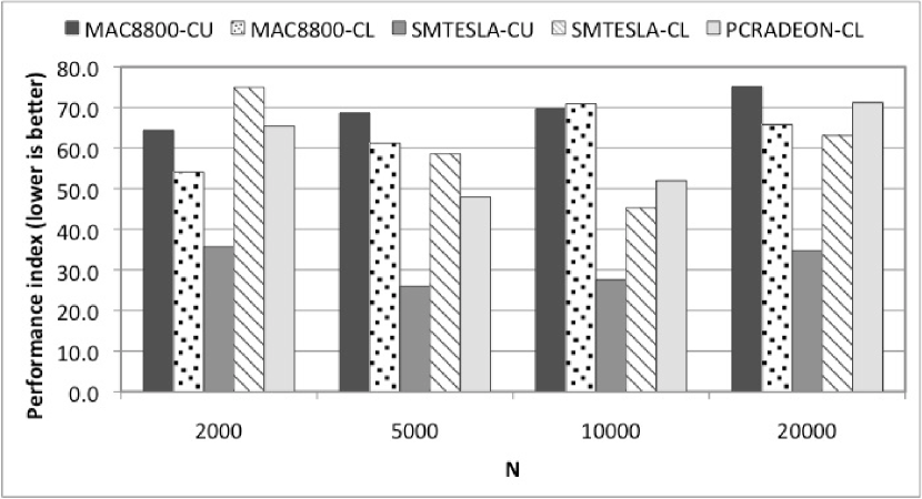
Figure 1: Performance index [measured execution time scaled by $(N/1000)^{3/2}$] for the NBODY1 code using CUDA (MAC8800-CU, SMTESLA-CU) and OpenCL (MAC8800-CL, SMTESLA-CL, PCRADEON-CL) kernels to directly calculate the interparticle forces, for varying system sizes. Lower performance index is better.

Results for the PCRADEON system running NBODY1 using an OpenCL kernel are also shown in Figure 1: its performance is within 10 per cent of that of the OpenCL kernel executing on the SMTESLA system. Considering that the ATI HD 5970 card retails for less than half the price of the Tesla C1060 card, and we have only used one of its two GPUs in this test, this is an outstanding result. Using both GPUs on the ATI HD 5970 can be expected to deliver performance at the level of the SMTESLA system using a CUDA kernel, for jobs that fit in the smaller memory ($<2$ GB) of the ATI card. There is clearly now a choice of hardware and software vendor for scientific computing using GPUs. Choosing OpenCL does not bestow a significant performance degradation compared to CUDA, and opens up additional options in GPU hardware for astronomy.

3 A GPU Programming Philosophy

Having considered the merits of CUDA and OpenCL for developing GPU-enabled astronomical software, we now consider a related question: for a given computational problem that has been identified as suitable for a GPU which version of the algorithm should be written or adapted for GPU? We present here a GPU-programming philopsophy based on brute force implementations.

3.1 Benefits of Brute Force

As a starting point for our GPU programming philosophy, we consider results from Thompson et al. (2010) and Bate et al. (2010) for the specific case of gravitational microlensing ray-shooting. Microlensing is the study of the gravitational deflection of light by compact lens masses within more massive, extended, lens galaxies; ray-shooting is a computational technique that follows light rays backwards from an observer, through a system of lenses that deflect the light rays, and onto a grid in the source plane. This grid, or magnification map, is then used to make statistical comparisons with microlensing observations.

The ‘industry standard’ ray-shooting method for single-core CPU uses a sophisticated tree-code (Wambsganss 1990; 1999). A tree hierachy is used to approximate the mass distribution as a collection of pseudo-lenses, in order to avoid the computational requirements of a direct summation over all lenses. This approach was originally introduced to microlensing two decades ago due to the unfeasibly long processing times (i.e. months to years) that the conceptually simpler, brute force computation using all lenses, would take on the best single-core CPUs available at the time. However, ray-shooting is inherently parallel – each light ray can be deflected independently of all other light rays, and the deflection due to each microlens adds linearly – thus making it an ideal candidate for a GPU implementation. Today, a high-resolution brute force calculation can be achieved in a matter of hours on a GPU. Moreover, with an NVIDIA Tesla S1070 unit, Thompson et al. (2010) achieved billion-particle microlensing calculations at over 1 teraflop/s and runtimes of a few days.

Bate et al. (2010) compared the single-core tree code (CPU-T) with the brute force approach on GPU (GPU-D where D = direct) over a range of astrophysically-motivated parameter space. Overall, runtimes using GPU-D were found to be no worse than for CPU-T: indeed, for certain combinations of parameters, GPU-D was a factor of a few faster. The implementation time for GPU-D using CUDA was quite short – a matter of weeks – compared to the anticipated time of several months to implement a working, optimised tree code.

What we infer from this case is that a naïve, simple to implement, and more accurate brute force solution is highly competive with a clever, complex, fast, trusted, industry standard code. Since its first release, the CPU-T code has not required significant modification in order to achieve faster processing times. Instead, it has been able to rely almost solely on the Moore’s Law increase in processing speed (and a corresponding growth in CPU memory at reduced cost). However, the plateau in CPU clock rates means that no additional performance improvement can occur for CPU-T in its present form. GPU-D is now ready to take advantage of the anticipated increases in GPU speeds in the years ahead, with no additional code development required. The massively parallel GPU architecture means that a brute force approach that was not feasible even a decade ago is now highly competitive with the algorithmically-complex approach. However, the latter was the only approach that was feasible for single-core CPU computing.

The Bate et al. (2010) result suggets an intriguing approach to GPU programming that we encourage other early adopters to consider. In order to adapt code to GPU, the two main alternatives are:

1. Take existing code and port it as is to GPU. This is likely to be a time-consuming task, as many aspects of complex implementations do not match well with the hardware architecture and memory management requirements of current GPUs; or

2. Think about what the code is currently doing and why [e.g. using an algorithm analysis approach as in Barsdell et al. (2010)].

If the latter reveals that a complex algorithm was being used in order to overcome a pre-existing hardware (i.e. single-core CPU) limitation, consider the advantages of a brute force approach. This may entail looking back to how a problem was originally posed, and taking the simple solution – provided it exhibits the required massive parallelism in computation that is suited for GPU.

Significant processing speed-ups can be obtained by going beyond a naïve implementation, but at the same time, a simple algorithm may yield unexpected speed-ups by over-computing. A case in point is the pairwise force calculation in direct $N$-body gravity simulations: saturation of GPU threads can be achieved by introducing additional particles with zero mass, and by explicitly calculating the pairwise forces $F_{ij}$ and $F_{ji}$, even though $F_{ij}=F_{ji}$ (Belleman et al. 2008). Aubert & Teyssier (2010) describe their use of an explicit time integration method for solving the equations of radiative transfer, taking advantage of GPU acceleration to remove a limitation that this approach would otherwise introduce.

Based on experiences so far, simples codes that are more accurate, more intuitive, and easier to implement for GPU, may result in runtimes that are already no worse than the best currently available (i.e. single-core) codes. We propose that brute force techniques where the programmer does not need to be as aware of computer science techniques, using algorithms that will hopefully map to a more obvious implementation on GPU, and which can be achieved over a short period of time (see section 3.3), are a sensible starting point for early adoption. In the longer term, once programmers have mastered the details of stream processing, and if the speed-up offered by a brute force solution is still not sufficient or scales poorly with the problem size, more sophisticated solutions can of course be implemented.

3.2 Brute-force multi-dimensional minimisation

To further test this philosophy, we consider a common task in astronomy: finding the global minimum of a multi-dimensional dataset. Standard techniques, such as steepest descent, simulated annealing or the simplex method (described below), attempt to limit the number of function evaluations required to obtain the minimum. While convergence to a solution can occur rapidly, there is no certainty that the global minimum has been obtained, rather than a local minimum. Moreover, solutions are often strongly dependent on the starting point for evaluation. Whereas techniques exist to find starting values that bracket the location of a minimum for one-dimensional functions, no such bracketing techniques exist for the general multi-dimensional case.

3.2.1 Downhill simplex minimisation

A popular multi-dimensional minimisation technique is the downhill simplex method (DSM), introduced by Nelder & Mead (1965). A practical implementation of this algorithm is is provided with the GNU Scientific library (GSL) as the function gsl_multimin_fminimizer_nsimplex. DSM is a very general multi-dimensional minimisation algorithm, as it does not depend on knowledge of the derivatives of a function (such as is required for the steepest descent algorithm), and hence is appropriate for a wider range of applications. DSM works as follows: based on an initial guess at a solution, $\mathbf{p}_{0}$, an additional $N$ vectors are generated using a stepping vector, $\mathbf{s}$. An $N$ dimensional simplex is constructed from these $N+1$ vectors as vertices, and the function evaluated at each vertex. A set of geometrical transformations are applied to the simplex in an attempt to span the minimum value, at which point the simplex contracts in size. This process is continued iteratively until a stopping criterion is reached.

As a demonstration of the difficulties associated with using DSM, consider the following well-behaved function in two-dimensions:

$$f(x,y)=\frac{\sin(x)\cos(y)}{\sqrt{1.0+x^{2}+y^{2}}}$$ (1)

which is plotted in Figure 2. As the visualisation ably demonstrates, there is one unique global minimum in the range $x\in[-10,10],y\in[-10,10]$, at $(x,y)=(-1.11,0.0)$ and a number of local minima.

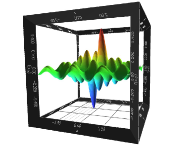
Figure 2: Surface representing the function $f(x,y)=\left[\sin(x)\cos(y)\right]/\sqrt{1.0+x^{2}+y^{2}}$. A rainbow colour-range (blue to red) is used to highlight function values. Three-dimensional visualisation is perhaps the easiest way to identify global minima and maxima for (well-behaved) two-dimensional functions!

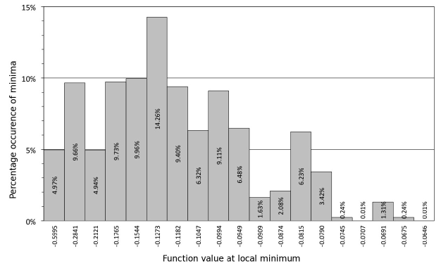
Figure 3: Distribution of minima found by GSL simplex routine for minimisation of equation (1), with starting values in the range $[-10,10]$ for $(x,y)$. Results based on executing code $10^{4}$ times. The actual global minimum is only found in $\sim 5\%$ of runs.

We implemented a wrapper for the DSM function in C, and ran $10^{4}$ iterations with random starting values for $(x,y)$ over the range $[-10,10]$. Total runtime for $10^{4}$ DSM solutions on a Xeon 5138 processor at 2.33 GHz was 0.4 s. Figure 3 shows the distribution of minima returned by the simplex routine. While DSM does indeed find the global minimum, it only achieves this in $5\%$ of cases.

Next, we trial a $5$-dimensional function

$$g(x,y,z,v,w)=\frac{\sin(x)\cos(y)\sin(z)\cos(v)\sin(w)}{\sqrt{1+x^{2}+y^{2}+z^{2}+v^{2}+w^{2}}},$$ (2)

which cannot be visualised as easily as for equation (1). However, by noting the symmetries $x\leftrightarrow z\leftrightarrow w$ and $y\leftrightarrow v$, we can consider the function:

$$h(u)=\frac{\sin^{3}(u)}{\sqrt{1+3u^{2}}},$$ (3)

which has a minimum at $u=-1.36672$, and deduce that there are four global minima at $(y,v)=(0,0)$ and $(x,z,w)$ as listed in Table 1.

Table 1: Global minima of the five-dimensional function of equation (2) occuring when $y=v=0$.

$x$	$z$	$w$	$f(x,y,z,v,w,)$
-1.36672	1.36672	1.36672	-0.365412
1.36672	-1.36672	1.36672	-0.365412
1.36672	1.36672	-1.36672	-0.365412
-1.36672	-1.36672	-1.36672	-0.365412

As before, the DSM code was executed $10^{4}$ times. Average runtime (over 10 runs) on the same CPU architecture as used previously was 1.97 s. For the five-dimensional function, one of the four global minima was only found in 0.03 $\%$ of cases.

As a simple modification, we enable the code to find successively lower values. Starting with an initial guess, DSM converges to a minimum value. A new starting point is chosen, and the solution is compared to the previous best minimum. This process continues until no lower minimum has been found after 100 iterations. This change increased the runtime to 5.23 seconds (average over 10 runs), and resulted in one of the four global minima being found in $0.13\%$ of runs.

An alternative strategy is to reduce the range for starting guesses, although in general, we might not know a priori what an appropriate (reduced) range is. Here, by choosing starting values in the range $[-5,5]$, and using the additional iteration step, our code returns a correct global minimum in $3.7\%$ of runs. A secondary effect here is a slight reduction in runtimes (4.8 s).

We have now demonstrated the difficulties with using an approximate method, such as DSM, for minimimisation of a well-behaved function. Our intent is not to provide a detailed analysis of how to improve performance of DSM, but to present a starting point for considering an alternative minimisation technique suitable for GPU: brute-force computation over a search domain.

3.2.2 Brute-force minimisation

In brute-force method (hereafter, BFM) minimisation, function values are evaluated on a grid of points in multi-dimensional parameter space. The resulting array of function values is searched or sorted to identify the minimum (or minima). The principal characteristic of this approach is that the quality of the solution—how close the result is to the real minimum (or minima)—depends on the resolution of the grid. In general, a finer grid yields a grid point (or set of grid points) closer to the true global minimum (minima). However, for real-world minimisation, minima will rarely align exactly with a grid point and consequently, unlike DSM, the BFM on its own may not yield the exact minimum.

What BFM can do though is identify the location, with known uncertainty of one-half of the grid spacing in each direction, of physically meaningful minima. By this we mean minima that are smooth with respect to the selected grid resolution, or put another way, minima that are well-behaved over the neighbouring grid cells. A sharp negative spike, confined in the multi-dimensional parameter space to a hypervolume smaller than a grid cell, cannot reliably be identified by brute-force; i.e. high-frequency features may be missed by the sampling of the parameter space.

Happily, for many real-world minimisation problems, especially those using measured data, it is actually quite reasonable and straightforward to set a physically meaningful resolution for searching parameter space. For example, consider fitting a Gaussian profile to a radio continuum image of a galaxy, with the position, width and amplitude parameters of the Gaussian to be determined. In most cases, position will be over-sampled at one-tenth of the resolution (beam size) of the image (although for extremely bright sources needing the best astrometry this could be refined); width would be sufficiently sampled in multiples of one-fifth the beamsize; and amplitude in multiples of one-fifth of the image noise. While this sampling implies a desired precision in the final fit, if subdividing the grid much finer than this yields substantially different solution(s), it is likely to be due to unphysical artefacts in the image (e.g. sharp spikes from interference or noise outliers, which are not convolved with the observing beam) rather than genuine signals of interest.

Minima found by brute-force sampling of parameter space can be used in their own right, or used as initial guesses for a method like DSM which could refine the solution (i.e. move it off the grid and towards the exact minimum). BFM minimisation can easily accommodate a priori conditions on the parameter search space, such as invalid regions (which can be masked out from the search) or parameters requiring varying resolution (e.g. using log sampling).

To explore the feasiblity of BFM minimisation using GPUs, we implemented the evaluation of equation (2) over a defined parameter space using an OpenCL kernel and driver program. For simplicity, all five variables were sampled over the domain $(-5,5)$ sampled at $N$ points; a total of $N^{5}$ function evaluations are required. For a given triplet $(x_{i},y_{j},z_{k})$, the kernel was programmed to sequentially evaluate the function over all $(v,w)$, a total of $N^{2}$ evaluations, and return the vector $(x_{i},y_{j},z_{k},v_{\rm min},w_{\rm min})$ and value $g_{\rm min}(x_{i},y_{j},z_{k})$ where the minimum function value was identified for the triplet $(x_{i},y_{j},z_{k})$. The kernel was deployed over a 3-dimensional work block $\mathcal{B}$ of size $(N,N,N)$, itself divided into work groups of size $(N,1,1)$. The driver program received $N^{3}$ values of $g_{\rm min}(x,y,z)$ at the completion of the kernel invocation, and used sequential CPU code to identify the global minimum and its location.

We measured the time taken to evaluate the test function for $N$ in the range 32–160. We used the MAC-8800 and PCRADEON systems as previously described, as well as a quad-core Intel Nehalem i7 930 Xeon system (PCXEON4) running a standalone C implementation (five nested loops over the $x,y,z,v,w$ parameter axes) of the brute force calculation. Figure 4 presents the results. For this compute-bound problem, the PCRADEON system (using 1 GPU) outperforms the PCXEON4 system by around 25 times, and can evaluate the function ($g$) at a rate of $\sim 10^{9}$ evaluations per second. Using both GPUs on the PCRADEON system would double this speed.

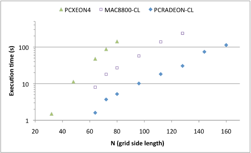
Figure 4: Measured execution time for the brute-force evaluation of equation (2) on a $N^{5}$-cell grid for a quad-core Xeon processor (PCXEON4) and OpenCL (MAC8800-CL, PCRADEON-CL) kernels. Lower execution time is better.

As previously noted, equation (2) has multiple minima, yet it is highly improbable that the grid used by the BFM exactly aligns with any of them. However, provided the grid is sampled finely enough, BFM minimisation will identify a point close to one of the four global minima, as the minimal point on the grid, hereafter $P_{b}$. As the sampling of the grid increases (i.e. as $N$ increases) the overall expectation is that $P_{b}$, and the function evaluated at that point, $g(P_{b})$, will approach the position and value of (one of) the global minima respectively. However this approach is not necessarily piecewise continuous because the minimum function evaluation on the grid will likely flip-flop from side-to-side of local or global minimum as $N$ is increased.

Figure 5 illustrates the convergence towards an acceptable solution for the test function with increasing subdivision of parameter space—for $N\simeq 100$, the global minimum value is accurate to $\sim 0.5$ per cent and the position is within $\sim 1$ per cent of one of the known global minima positions. In the real world, with e.g. measurement noise and resolution effects added to this dataset, $N$ would be sensibly limited by known properties of the data.

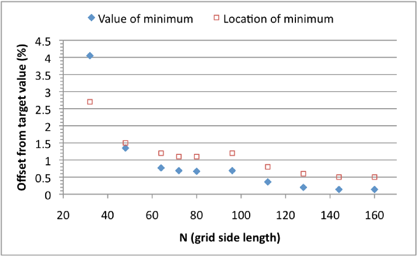
Figure 5: Convergence of BFM minimisation to the value and location of a global minimum of equation (2) as a function of the grid side length $N$. The value offset is expressed as a percentage of the target minimum value; the position offset as a percentage of the diagonal length of the 5-dimensional parameter space.

To compare the standard downhill simplex method to the brute force approach for minimising the test function, we consider what can be achieved by each method in 10 s:

• DSM (on the Xeon 5138 CPU) has a $7.7$ per cent strike rate in identifying exactly one of the four global minima (i.e. it has a $92.3$ per cent likelihood of not identifying one of the global minima!); and

• BFM (on the PCRADEON-CL system) identifies a lowest value within $0.7$ per cent of the known global minimum value, lying closer than $1.2$ per cent of the diagonal length of the parameter space to one of the known global minima locations.

While BFM minimisation could be re-run at higher resolution in a sub-volume of parameter space around minima found on lower resolution grid/s to improve the accuracy of its results, a hybrid DSM-BFM method is obviously suggested. Using for example the $\sim 100$ lowest points found in the brute force evaluation of the function $g$ over the 5-dimensional parameter space with $N=64$, as initial guesses for the downhill simplex method, we obtain a method which can readily identify all four global minima for the function $g$, exactly, in just a few seconds.

Or intent in this section has been to demonstrate that a brute force approach is a practical starting point for a GPU, which gives a significant speed-up compared to a CPU (Figure 4), and may indeed overcome some of the existing limitations with the optimised alternatives. Implementating BFM minimisation using CUDA or OpenCL is straightforward, whereas efficient coding of a more complex minimisation algorithm for a GPU is likely to be a time-consuming task – and would result in the same issues with identifying local rather than global minima. The brute force approach could indeed be used in a multi-scale fashion to obtain higher accuracy, e.g. for each local minima, repeat the brute force evaluation but on a higher resolution local grid, or for providing the starting points for an alternative techinque.

3.3 Time to Science

Since there is an overhead in preparing code to run effectively and optimally on GPU, it is worth considering how much time is spent on programming versus the actual speed-ups. For the astronomer, whose primary interest is their ability to advance knowledge through computation, rather than advancing knowledge of the computational technique, we can consider a time to science, $T_{\rm science}$, to aid decisions regarding adoption of GPU:

$$T_{\rm science}=T_{\rm learn}+T_{\rm implement}+T_{\rm run}+T_{\rm analysis}.$$ (4)

Here, $T_{\rm learn}$ is the time taken to learn the fundamentals of a programming approach (CPU or GPU), $T_{\rm implement}$ is the time to implement a specific programmatic solution, $T_{\rm run}$ is the runtime of the code, and $T_{\rm analysis}$ is the time taken to analyse the outputs in preparation for future work or publication. A GPGPU approach is a desirable or beneficial in cases where $T_{\rm science}(GPU)\ll T_{\rm science}(CPU)$, but can we estimate how each factor is likely to contribute?

The most apparent advantage of GPGPU, and the most significant factor in $T_{\rm science}$, is the expectation that

$$T_{\rm run}(GPU)\ll T_{\rm run}(CPU).$$ (5)

This has been demonstrated for a growing range of GPU-astronomy applications, with $10-100\times$ speed-ups in processing time. If this condition is not met, there is little to be gained from a GPU implementation.

For a given number of outputs, we expect that

$$T_{\rm analysis}(GPU)\sim T_{\rm analysis}(CPU),$$ (6)

as the analysis time should not be affected by the computational runtime. If we consider a scenario where faster GPU runtimes are used primarly to produce more outputs than are possible with CPU, then the total analysis time will grow.

Based on our experiences, we suggest that

$$T_{\rm learn}(GPU)>T_{\rm learn}(CPU),$$ (7)

and may indeed be

$$T_{\rm learn}(GPU)\gg T_{\rm learn}(CPU).$$ (8)

In general, the average astronomer-programmer does not have training in parallel programming techniques - we anticipate that this situation may be resolved in the years ahead as multi- and many-core programming makes it way into undergraduate courses, but this may be a major factor in the short term. While it has been possible for many code-writing astronomers to remain unaware of the hardware configuration of a CPU (beyond knowing the total available memory), optimising code for GPUs requires a more complete knowledge of issues such as available memory bandwidth, and appropriate allocation of data between register, device and shared memory spaces (e.g. Che et al. 2008; Christadler & Weinberg 2010).

Regardless of architecture, we assert that:

$$T_{\rm implement}({\rm simple})\ll T_{\rm implement}({\rm complex})$$ (9)

namely that is faster and easier to implement a simple, brute force solution, than to code a more complex algorithm. As our initial investigations suggest, such an approach can still result in:

$$T_{\rm run}(\mbox{GPU-simple code})\leq T_{\rm run}(\mbox{CPU-complex code}).$$ (10)

Assessing the combined effects of these factors is challenging, however, we suggest that $T_{\rm science}$ will be smaller for simple to implement, brute-force GPU codes in cases, despite the overheads in learning to appropriate GPU programming techniques. Of course, as with traditional CPU programming, these techniques only need to be learnt once, and can then be applied to a range of computational problems in the future. In the same way that single-core CPU codes have benefitted from Moore’s Law, once a simple GPU code is available, it can also take advantage of the anticipated processing speed-ups that will occur in future generations of GPU hardware, regardless of whether additional time/effort is invested to develop a more optimised ‘complex on GPU’ solution.

4 Other considerations

We now briefly comment on several additional factors that early adopters should be aware of: issues of performance and precision, tools to aid in profiling and optimising code, and the role of third-party GPU-code libraries and GPU-enhanced programming environments.

4.1 Performance, Precision and Optimisation

Graphics processing generally only requires single precision floating point calculations, but astronomy computation may require double precision computation in order to achieve sufficient numerical accuracy. Presently, there is a big performance difference between single-precision (SP) and double-precision (DP) computation, as GPU hardware has fewer DP processors. In some cases, DP emulation can be achieved by packing a DP value (64 bit) into two SP floats (32 bit), resulting in two times increase in precision – this approach was used by Gaburov et al. (2009) in their SAPPORO N-body code. This is likely to only be a short-term limitation for GPUs, as increased DP performance is under consideration by GPU vendors (e.g. while SP speeds have increased overall, in the move from the NVIDIA Tesla S1070 to the newer Fermi hardware, DP speeds have improved from 1/8 to 1/2 the SP rates). An additional factor that may limit longer calculations is the availability of error correcting memory (ECC), which is able to mitigate failures due to memory errors from interference (including cosmic rays) or hardware problems [see Schroeder et al. (2009) for an empirical study]. NVIDIA’s Fermi cards now support EEC, but with a slight decrease in processing performance when this mode is enabled, and a reduction in the amount of allocatable GPU memory.

Writing working GPU code is not the same as writing optimised, efficient GPU code. A simple GPU implementation of a parallel algorithm, such as those presented here, may require several iterations in order to reach a sufficiently optimised version. Factors of $2-10\times$ in speed can be achieved quickly, but reaching $100\times$ does require effort and expertise. Tools such as the CUDA occupancy calculator can help to improve speed through improved use of GPU memory spaces and ensuring that all stream processors are being highly utilised. We caution that quoted peak speeds for GPU hardware are primarily for graphics-like calculations (e.g. dual issuing of a multiplication and addition per clock cycle for single-precision). A more realistic outcome is to achieve about 1/4 to 1/2 of the quoted peak performance, at best, but it is strongly problem-dependent.

While many astronomer-programmers may be familiar with techniques for debugging code, they may be less aware of the existence or importance of code profiling. A software profiler examines run-time characteristics of codes, including memory allocation, time spent executing functions, and the frequency of their execution. Profiling can help identify code sections that may benefit from optimisation. CUDA and both the NVIDIA and AMD OpenCL implementations provide visual profilers as part of their SDKs. Investing time learning to use these tools effectively may have a beneficial impact on $T_{\rm science}(GPU)$.

4.2 Third-party libraries and programming environments

From our own experience, there is a general trend for astronomers to re-implement code or algorithms that may already exist in third-party libraries. Obvious exceptions to this include the use of the FFTW Fourier transform libraries, the PGPLOT graphics subroutine library library, and code fragments or implementations from Numerical Recipes Software. A growing number of GPU-oriented libraries are now available, including the CUDA Data parallel Primitives Library (CUDPP) that provides primitives for common tasks like sorting and building data structures, and CUFFT – NVIDIA’s own CUDA FFT library.

Alternatives to programming code in CUDA or OpenCL, optimised for execution on a GPU, include GPU-enabled enhancements to widely used interactive environments and scripting languages such as the Interactive Data Language (IDL), Mathematica, and the Python programming language. For example, the CUDA-basd GPULib by Tech-X Corporation allows IDL scripts to access a GPU for common mathematical functions and processes (e.g. interpolation, correlation and parallel geneneration of random numbers). Similarly, PyCUDA and PyGPU are two implementations that enable GPU computing within Python. Moreover, compiler-based solutions such as the HMPP Workbench, aim to hide the details of GPU code development through the use of OpenMP-like directives in standard codes. As with the case of chosing OpenCL in preference to CUDA, there is likely to be some processing overhead in using one of these solutions, but they do provide a simpler, high-level access to GPU that may be preferable for many types of applications.

5 Concluding Remarks

In this paper, we have highlighted some of the benefits and limitations of early adoption of GPGPU for astronomy. While there are risks and significant effort may be required to prepare codes, in many cases the benefits will outweigh the limitations. A preferred outcome for astronomers is a majority of time and effort spent on scientific outcomes rather than software development.

The promise of the OpenCL standard, is to provide opportunities for hardware-agnostic coding. OpenCL seems to present a good amount of flexibility for implementation, rather than using a native API (such as CUDA for NVIDIA), without a significant decrease in processing speed. Furthermore, we suggest that for certain classes of scientific computations a step backwards to consider simple, brute force solutions that were not feasible for CPU, may instead reduce software development times. The resulting codes may already be ‘no worse’ than the best single-core alternatives, and may even be more accurate, or overcome limitations of existing optimised approaches. Lessons learnt in starting with brute force solutions can then help researchers to determine whether a longer-term solution does indeed warrant the effort of implementing a more sophisticated alternative.

While running codes faster may be an end in itself, faster computation means that there is more time to explore parameter space. This might include running models with different parameters, or running repeat models with different random seeds in order to build up a more robust statistical sample. Additionally, GPUs provide opportunities to tackle computational problems that are still not feasible on single core CPU or traditional multi-core computing clusters, at a greatly reduced cost.

Not all applications require GPUs, so some time and effort should be invested in understanding the types of problems that will really achieve the greatest benefit. For example, telescope control software does not parallelise well, if at all, but the highly parallel nature of Fourier transformation, used extensively in astronomy, makes it an ideal candidate for GPGPU. Indeed, there are problems, such as the conceptually simple process of generating a histogram from data values, that are easy to implement on a CPU, but which become unnecessarily complex when attempting to find a parallel solution. Computational tasks compatible with a stream processing paradigm, i.e. many individual data-streams requiring identical computations, are candidates for moving from the CPU to the GPU. Fortunately, a high degree of data parallelism is present in many astronomy scenarios (e.g. the use of the CLEAN algorithm in radio astronomy, which takes advantage of data parallelism in the spectral domain).

Identification of relevant astronomy computations is the first step towards implementation on GPU. Barsdell et al. (2010) propose an approach based on algorithm analysis, whereby common processing tasks are matched to a taxonomy of algorithms. Despite its obvious application to GPGPU development, this approach may provide insight into improvements and optimisation for single-core and multi-core CPU codes. An improved understanding of the parallelism in existing astronomy codes and algorithms can lead to simple optimisation, such as identifying sections of code that would benefit from the trivial parallelisation on multi-core architectures possible with OpenMP. Indeed, in some cases, the simpler shared-memory programming model provided by OpenMP may provide a sufficient processing improvement without resorting to a GPU solution. For a code to be moved to a GPU, rather than using OpenMP on a modern quad-core architecture, it typically needs to present a 20-30x speed-up over the single-core solution. The counter argument is that GPUs remain significantly cheaper on a $/gigaflop basis than a sufficiently multi-core computer (e.g. $>24$ cores) that would provide the same processing performance.

We emphasise that skills in parallel or stream processing programming techinques are not widespread amongst astronomy graduates or graduate students, and the ‘supervisor teaching the student to code’ may no longer be feasible. It is often a difficult decision to choose between spending limited research resources on direct (travel, graduate student stipends, postdoctoral salaries) versus indirect research costs (programmers who may not have, nor actually seek, scientific training). However, it will not be feasible for astronomers to prepare for GPU-based HPC facilities without some investment in training on parallel programming techniques.

The long-term role of the GPU is still unknown: whether they will remain as a computational coprocessor, or if multi-core CPUs will grow to become more GPU-like. There may be other radical changes in hardware in the years ahead, such as the experimental 48-core Intel single-chip cloud computer announced in 2009. The recent demise of Intel’s Larabee consumer GPU chip, a hybrid CPU and GPU, with features such as cache coherency across all cores and greater flexibility in computation, may have delayed resolution of this issue for at least a few more years. While these short term changes may lead to some redundancy in code development effort, awareness of the fundamental differences between CPU and GPU programming and execution should provide insight into problem solving for future highly parallel architectures. Moreover, we anticipate that the move to astronomical GPGPU may not be limited to HPC facilities, but will ultimately encompass desktop and notebook supercomputing.

GPGPU represents a natural new direction for astrophysical HPC. Adoption of a radical new processing architecture, and the correspoding required change in approach to software development, is worthwhile if our understanding of the universe advances at an accelerated rate. We remain enthusiastic about the prospects for GPGPU in astronomy.

References

- Aarseth (1999) Aarseth, S.J., 1999, PASP, 111, 1333
- Aubert & Teyssier (2010) Aubert, D., Teyssier, R., 2010, arXiv:1004.2503 [astro-ph]
- Aubert et al. (2009) Aubert, D., Amini, M., David, R., 2009, Lecture Notes in Computer Science, 5544/2009, 874
- Barsdell et al. (in prep) Barsdell, B.R., Fluke, C.J., & Barnes, D.G. 2010, MNRAS, accepted June 2010, arXiv:1007.1660 [astro-ph]
- Bate et al. (2010) Bate, N.F., Fluke, C.J., Barsdell, B.R., Garsden, H., & Lewis, G.F. 2010, New Astronomy, 15, 726
- Belleman et al. (2008) Belleman, R.G., Bédorf, J., & Portegies Zwart, S.F. 2008, NewA, 13, 103
- Che et al. (2008) Che, S., Boyer, M., Meng, J., Tarjan, D., Sheaffer, J., & Skadron, K. 2008, Journal of Parallel and Distributed Computing, 68, 1370
- Christadler & Weinberg (2010) Christadler, I., & Weinberg, V. 2010, arXiv:1001.1902 [cs.PF]
- Elsen et al. (2007) Elsen, E., Vishal, V., Houston, M., Pande, V., Hanrahan, P., & Darve, E. 2007, arXiv:0706.3060v1 [cs.CE]
- Ford (2008) Ford, E.B. 2008, NewA, 14, 406
- Fournier & Fussell (1988) Fournier, A., & Fussell, D. 1988, ACM Transactions on Graphics, 7, 103.
- Gaburov (2009) Gaburov, E., Harfst, S., & Portegies Zwart, S. 2009, NewA, 14, 630
- Hamada & Iitaka (2007) Hamada, T., & Iitaka, T. 2007, arXiv:astro-ph/0703100v1
- Harris et al. (2008) Harris, C., Haines, K., & Staveley-Smith, L. 2008, ExA, 22, 129
- Karimi et al. (2010) Karimi, K., Dickson, N.G., & Hamaz, F. 2010, arXiv:1005.2581v1 [cs.PF]
- Khanna & McKennon (2010) Khanna, G., & McKennon, J. 2010, arXiv:1001.3631v1 [astro-ph]
- Kirk & Hwu (2010) Kirk, D.B., & Hwu, W.-m., W. 2010, Programming Massively Parallel Processors (Burlington:Morgan Kauffman Publishers)
- Larus & Gannon (2010) Larus, J., & Gannon, D. 2010, in The Fourth Paradigm: Data-Intensive Scientific Discovery, ed. T. Hey, S. Tansley, & K. Tolle (Microsoft Research), 125
- Moore et al. (2008) Moore, A.J., Quillen, A.C., & Edgar, R.G. 2008, arXiv:0809.2855v1 [astro-ph]
- Nelder & Mead (1965) Nelder, J.A., & Mead, R. 1965, Computer Journal, 7, 308
- Nyland et al. (2004) Nyland, L., Harris, M., & Prins, J.F. 2004, in ACM Workshop on General-Purpose Computing on Graphics Processors (Poster), C-37
- Nyland et al. (2008) Nyland, L., Harris, M., & Prins, J.F. 2008, GPU Gems 3, Addison-Wesley, ch. 31, 677
- Ord et al. (2009) Ord, S., Greenhil, L., Wayth, R., Mitchell, D., Dale, K., Pfister, H., & Edgar, R.G. 2009, arXiv:0902.0915 [astro-ph.IM]
- Owens et al. (2005) Owens, J.D., Luebke, D., Govindaraju, N., Harris, M. Krüger, J., Lefohn, A.E., & Purcell, T.J. 2005, Computer Graphics Forum, 26), 80
- Portegies Zwart et al. (2007) Portegies Zwart, S.F., Belleman, R.G., & Geldof, P.M. 2007, NewA, 12, 641
- Schaaf & Overeem (2004) Schaaf, K.V.D., & Overeem, R. 2004, ExA, 17, 287
- Schive et al. (2007) Schive, H.-Y., Chien, C.-H., Wong, S.-K., Tsai, Y.-C., & Chiueh, T. 2007, NewA, 13, 418
- Schroeder et al. (2009) Schroeder, B., Pinheiro, E., Weber, W.-D., 2009, in SIGMETRICS ’09: Proceedings of the eleventh international joint conference on Measurement and modeling of computer systems, 193
-
Simpson etl a. (2008)
Simpson, A., Bull, M., & Hill, J. 2008, PRACE Deliverable D6.1, available
from http://www.prace-project.eu/documents/
public-deliverables-1/ - Szalay et al. (2008) Szalay, T., Springel, V., & Lemson, G. 2008, arXiv:0811.2055v2 [cs.GR]
- Thompson et al. (2010) Thompson, A.C., Fluke, C.J., Barnes, D.G., & Barsdell, B.R. 2010, NewA, 15, 16
- Tomov et al. (2003) Tomov, S., McGuigan, M., Bennett, R., Smith, G., & Spiletic, J. 2003, arXiv:cs/0312006
- Venkatasubramanian (2003) Venkatasubramanian, S. 2003, in SIGMOD Workshop on Management and Processing of Massive Data, arXiv:cs/0310002
- Wayth et al. (2007) Wayth, R., Dale, K., Greenhill, L.J., Mitchell, D.A., Ord, S., & Pfister, H. 2007, AAS, 211, 1104