Statefinder diagnostic and stability of modified gravity consistent with holographic and new agegraphic dark energy

Abstract

Recently one of us derived the action of modified gravity consistent with the holographic and new-agegraphic dark energy. In this paper, we investigate the stability of the Lagrangians of the modified gravity as discussed in [M. R. Setare, Int. J. Mod. Phys. D 17 (2008) 2219; M. R. Setare, Astrophys. Space Sci. 326 (2010) 27]. We also calculate the statefinder parameters which classify our dark energy model.

Keywords: Dark energy; modified gravity; statefinder parameters; holographic dark energy; agegraphic dark energy.

1 Introduction

Nowadays it is strongly believed that the universe is experiencing an accelerated expansion. Recent observations from type Ia supernovae [1] in associated with Large Scale Structure [2] and Cosmic Microwave Background anisotropies [3] have provided main evidence for this cosmic acceleration. There are two ways to explain the current accelerated expansion of the universe. The first one is to introduce some unknown matter, which is called dark energy in the framework of general relativity.

On the other hand the nature of dark energy is ambiguous. The simplest candidate of dark energy is a cosmological constant with the equation of state parameter $\omega=-1$. However, this scenario suffers from serious problems like a huge fine tuning and the coincidence problem [4]. Alternative models of dark energy suggest a dynamical form of dark energy, which is often realized by one or two scalar fields. In this respect, dark energy components such as quintessence [5], K-essence [6], tachyon [7], phantom [8], ghost condensate and quintom [9], and so forth.

Although going beyond the above effective description requires a deeper understanding of the underlying theory of quantum gravity [10] unknown at present, physicists can still make some attempts to probe the nature of dark energy according to some basic quantum gravitational principles. An example of such a paradigm is the holographic dark energy scenario, constructed in the light of the holographic principle [11, 12, 13, 14]. Its framework is the black hole thermodynamics [20] and the connection (known from AdS/CFT correspondence) of the UV cut-of of a quantum field theory, which gives rise to the vacuum energy, with the largest distance of the theory [11]. Thus, determining an appropriate quantity $L$ to serve as an IR cut-off, imposing the constraint that the total vacuum energy in the corresponding maximum volume must not be greater than the mass of a black hole of the same size, and saturating the inequality, one identifies the acquired vacuum energy as holographic dark energy:

$$\rho_{\Lambda}=\frac{3c^{2}}{8\pi GL^{2}},$$ (1)

with $G$ the Newton’s gravitational constant and $c$ a constant. The holographic dark energy scenario has been tested and constrained by various astronomical observations [15, 16, 17, 18, 19] and it has been extended to various frameworks [21, 22, 23].

More recently a new dark energy model, dubbed agegraphic dark energy has been proposed. These models take into account the Heisenberg uncertainty relation of quantum mechanics together with the gravitational effect in general relativity. The agegraphic dark energy models assume that the observed dark energy comes from the spacetime and matter field fluctuations in the universe [24, 25, 26]. Since in agegraphic dark energy model the age of the universe is chosen as the length measure, instead of the horizon distance, the causality problem in the holographic dark energy is avoided. The agegraphic models of dark energy have been examined and constrained by various astronomical observations [27].

Another alternative approach to explain the universe’s late-time acceleration is modifying the General Relativity itself [28], and in the simplest case replace $R$ with $f(R)$ in the action which is well known as $f(R)$ gravity. Here $f(R)$ is an arbitrary function of scalar curvature. Although there are some works with related subjects on crossing of the phantom divide line in the framework of modified gravity [29, 30], but Ref.[31] was the first paper that has investigated a modified gravity model realizing $\omega$ across -1. The authors of Ref.[31] have shown an explicit model of modified gravity in which a crossing of the phantom divide can occur and relation between scalar field theories with property of $\omega$ crossing -1 and the corresponding modified gravity theories have been investigated. Observationally the possibility of phantom crossing was suggested by early supernova data sets [32] while the situation concerning present data is rather ambiguous [33].

In paper [34], using the holographic model of dark energy in spatially flat universe, one author of this paper has obtained equation of state for holographic dark energy density in framework of modified gravity for a universe enveloped by $R_{h}$ as the system’s IR cut-off. Also he has developed a reconstruction scheme for the modified gravity with $f(R)$ action. He could to obtain a differential equation for $f(R)$, the solution of this differential equation give us a modified gravity action which is consistent with holographic dark energy scenario. In [35] this investigation extended to new agegraphic dark energy model.

2 Holographic dark energy

The energy density of holographic dark energy is given by ($8\pi G=1$)

$$\rho_{D}=3c^{2}R_{h}^{-2},$$ (2)

where $c$ is a constant and $R_{h}$ is the future event horizon specified by

$$R_{h}\equiv a(t)\int\limits_{t}^{\infty}\frac{dt}{a^{\prime}}=a(t)\int\limits_{a(t)}^{\infty}\frac{da^{\prime}}{Ha^{\prime 2}}.$$ (3)

The critical energy density $\rho_{cr}$ is given by the following expression

$$\rho_{cr}=3H^{2},$$ (4)

which helps us to write the dimensionless density parameter for dark energy

$$\Omega_{D}=\frac{\rho_{D}}{\rho_{cr}}=\frac{c^{2}}{R_{h}^{2}H^{2}}.$$ (5)

Differentiating (3) and using (5), we are able to write

$$\dot{R}_{h}=HR_{h}-1=\frac{c}{\sqrt{\Omega_{D}}}-1.$$ (6)

The energy conservation equation for (any form of) dark energy is

$$\dot{\rho}_{D}+3H(1+\omega_{D})\rho_{D}=0.$$ (7)

Differentiating (2) w.r.t $t$ and using (5) yields

$$\dot{\rho}_{D}=-2\frac{\rho_{D}}{R_{h}}\Big{(}\frac{c}{\sqrt{\Omega_{D}}}-1\Big{)}.$$ (8)

Using (8) in (7) yields

$$\omega_{HDE}=-\frac{1}{3}-\frac{2}{3c}\sqrt{\Omega_{D}},$$ (9)

the equation of state parameter for the holographic dark energy.

3 Stability of modified gravity with HDE

It is shown in [34] that a modified gravity consistent with the holographic dark energy in flat space has the following form:

$$f(R)=C_{1}R^{u}+C_{2}R^{v}+\frac{c^{2}(1-h_{0})^{2}R}{2h_{0}^{2}},$$ (10)

where $h_{0}$ is a constant which is related to the scale factor as $a(t)=a_{0}(t_{s}-t)^{h_{0}}$, $t_{s}$ and $a_{0}$ are also constants. The expressions of $u$, $v$, $C_{1}$ and $C_{2}$ are discussed in [34].

For a phenomenological $f(R)$ model to be viable, it must meet a certain list of viability conditions [36]: classical and quantum stability which involves $f^{\prime}(R)>0$ and $f^{\prime\prime}(R)>0$ (the first positive derivative means that gravity is attractive and the graviton is not a ghost while the second positive derivative is used to avoid the Doglov-Kawasaki instability); stable Newtonian limit for all values of $R$; absence of deviations from general relativity and existence of a future de Sitter asymptote. We are interested here to check the stability of our $f(R)$ models only. The stability can be checked by calculating the double derivative of $f(R)$ in (10):

$$f^{\prime\prime}(R)\equiv\frac{d^{2}f}{dR^{2}}=C_{1}u(u-1)R^{u-2}+C_{2}v(v-1)R^{v-2}.$$ (11)

Now $f^{\prime\prime}(R)>0$ if $C_{1}>0$, $C_{2}>0$, $u>1$ and $v>1$. This case corresponds to stability while a negative double derivative results in instability. We are not interested in the later case. There are some suggestions that the instabilities associated with $f(R)$ action can be removed by adding quadratic and higher order terms along with the Ricci scalar $R$ [37]. Thus due to abundance of free parameters, the instabilities associated with $f(R)$ action are naturally alleviated. Note that when $f^{\prime\prime}(R)=0$ for a suitable choice of model parameters (e.g. $C_{1}=0=C_{2}$) then the theory reduces to general relativity and is of no interest here.

4 New agegraphic dark energy

The energy density of the new agegraphic dark energy is given by

$$\rho_{D}=3n^{2}\eta^{-2},$$ (12)

where $n$ is a constant and $\eta$ is the conformal time defined by

$$\eta=\int\frac{dt}{a}=\int\limits_{0}^{a}\frac{da^{\prime}}{a^{\prime 2}H}.$$ (13)

Using (12) and (4), we obtain

$$H\eta=\frac{n}{\sqrt{\Omega_{D}}}.$$ (14)

Differentiating (12), we get

$$\dot{\rho}_{D}=-\frac{2}{a\eta}\rho_{D}.$$ (15)

Using (15) in (7), we obtain

$$\omega_{NADE}=-1+\frac{2}{3an}\sqrt{\Omega_{D}}.$$ (16)

5 Stability of modified gravity with NADE

It is shown in [35] that a modified gravity consistent with the agegraphic dark energy in flat space has the following form:

$$f(R)=C_{3}R^{u}+C_{4}R^{v}+\frac{C_{5}}{R^{h_{0}-1}}.$$ (17)

The expressions of $C_{4}$ and $C_{5}$ are discussed in [35].

Now stability can be checked by calculating the double derivative of $f(R)$ in (17):

$$\frac{d^{2}f}{dR^{2}}=C_{3}u(u-1)R^{u-2}+C_{4}v(v-1)R^{v-2}+h_{0}(h_{0}-1)\frac{C_{5}}{R^{1+h_{0}}}.$$ (18)

Now $f^{\prime\prime}(R)>0$ if $C_{3}>0$, $C_{4}>0$, $C_{5}>0$, $u>1$, $v>1$ and $h_{0}>1$. This case corresponds to stability while a negative double derivative results in instability. We are not interested in the later case. It should be noted that the order of these coefficients should of the order of $H_{0}^{2}\simeq 10^{-66}eV^{2}$, so that the correction terms play their role at the present time to produce cosmic acceleration. We would also mention that at present there is no indication what should be the correct modification of the Einstein’s general relativity from the observations. On the other hand, some recent astrophysical observations of weak lensing and galaxy velocities indicate that general relativity is still the best fit of the astrophysical data [40]. The present considered models contain numerous parameters and observational data can constrain them only.

6 Statefinder diagnostic

In this section, we calculate the statefinder parameters for the above two models of dark energy. Sahni et al [41] introduced a pair of cosmological diagnostic pair $\{r,s\}$ which they termed as Statefinder. The two parameters are dimensionless and are geometrical since they are derived from the cosmic scale factor alone, though one can rewrite them in terms of the parameters of dark energy. Additionally, the pair gives information about dark energy in a model independent way i.e. it categorizes dark energy in the context of background geometry only which is not dependent on the theory of gravity. Hence geometrical variables are universal. Also this pair generalizes the well-known geometrical parameters like the Hubble parameter and the deceleration parameter. This pair is algebraically related to the equation of state of dark energy and its first time derivative.

The statefinder parameters $\{r,s\}$ are defined as [41, 42]

$$r\equiv\frac{\stackrel{{\scriptstyle...}}{{a}}}{aH^{3}},\ \ s\equiv\frac{r-1}{3(q-1/2)}.$$ (19)

Note that in the derivation of the above parameters, a spatially flat FRW spacetime is assumed. A useful alternative form of (19) is

$$r = 1-\frac{3}{2}\Omega_{D}\Big{[}\frac{\dot{\omega}_{D}}{H}-3\omega_{D}(1+\omega_{D})\Big{]},$$ (20)

$$s = \frac{-1}{3\omega_{D}}\Big{[}\frac{\dot{\omega}_{D}}{H}-3\omega_{D}(1+\omega_{D})\Big{]}.$$ (21)

One can immediately see that for cosmological constant with constant equation of state ($\omega_{D}=-1$), we have $\{1,0\}$. Moreover $\{1,1\}$ represents the standard cold dark matter model containing no radiation while Einstein static universe corresponds to $\{\infty,-\infty\}$ [43]. In literature, the diagnostic pair is analyzed for various dark energy candidates including holographic dark energy [44], agegraphic dark energy [45], quintessence [46], dilaton dark energy [47], Yang-Mills dark energy [48], viscous dark energy [49], interacting dark energy [50], tachyon [51], modified Chaplygin gas [52], $f(R)$ gravity [53] and dark energy model with variable constants [54] to name a few.

The dimensionless dark energy density parameter is [34, 35]

$$\Omega_{D}=\frac{1}{3H^{2}}\Big{[}f(R)-6(\dot{H}+H^{2}-H\frac{d}{dt})f^{\prime}(R)\Big{]},$$ (22)

where prime denotes differentiation w.r.t $R$. The above expression can be written as

$$\Omega_{D}=\frac{1}{3H^{2}}\Big{[}f(R)-6(\dot{H}+H^{2})F(R)+6HF_{,R}\dot{R}\Big{]},$$ (23)

where we have used the following relations

$$F(R)\equiv f^{\prime}(R),\ \ \frac{d}{dt}f^{\prime}(R)=f_{,RR}\dot{R}=F_{,R}\dot{R}.$$ (24)

We proceed to calculate statefinder parameters for the NADE. Substituting (23) in (16)

$$\omega_{NADE}=-1+\frac{2}{3\sqrt{3}anH}\sqrt{f(R)-6(\dot{H}+H^{2})F(R)+6HF_{,R}\dot{R}}.$$ (25)

We differentiate (16) w.r.t $t$ and obtain

$$\dot{\omega}_{NADE}=\frac{2}{3na}H\sqrt{\Omega_{D}}\Big{(}\frac{\dot{\Omega}_{D}}{2H\Omega_{D}}-1\Big{)}.$$ (26)

Differentiating (23) leads to

$$\dot{\Omega}_{D} = \frac{-2\dot{H}}{3H^{3}}\Big{[}f(R)-6(\dot{H}+H^{2})F(R)+6HF_{,R}\dot{R}\Big{]}$$ (27)

$$+\frac{1}{3H^{2}}[F\dot{R}-6(\stackrel{{\scriptstyle...}}{{H}}+2H\dot{H})F+6\dot{H}F_{,R}\dot{R}+6H(F_{,RR}\dot{R}^{2}+F_{,R}\ddot{R})].$$

Similarly, we obtain parameters for the HDE:

$$\omega_{HDE}=\frac{-1}{3}-\frac{2}{3\sqrt{3}cH}\sqrt{f(R)-6(\dot{H}+H^{2})F(R)+6HF_{,R}\dot{R}}.$$ (28)

$$\dot{\omega}_{HDE}=\frac{-1}{3c}\frac{\dot{\Omega}_{D}}{\sqrt{\Omega_{D}}}.$$ (29)

Using (16) and (26) in (20) and (21), we obtain

$$r_{NADE}=1-\frac{3}{an}\Omega_{D}^{3/2}\Big{[}1-\frac{\sqrt{\Omega_{D}}}{an}+\frac{\dot{\Omega}_{D}}{4H\Omega_{D}}\Big{]}.$$ (30)

$$s_{NADE}=\frac{2}{3an}\sqrt{\Omega_{D}}\Big{[}1-\frac{-1+\frac{\dot{\Omega}_{D}}{2H\Omega_{D}}}{-3+\frac{2}{an}\sqrt{\Omega_{D}}}\Big{]}.$$ (31)

Similarly we can obtain $\{r,s\}$ parameters for the HDE as

$$r_{HDE}=1-\frac{1}{2}\Omega_{D}\Big{[}-\frac{1}{cH}\frac{\dot{\Omega}_{D}}{\sqrt{\Omega_{D}}}+2\Big{(}1-\frac{4}{c^{2}}\Omega_{D}\Big{)}\Big{]}.$$ (32)

$$s_{HDE}=\frac{1}{3\Big{(}1+\frac{2}{c}\sqrt{\Omega_{D}}\Big{)}}\Big{[}-\frac{1}{cH}\frac{\dot{\Omega}_{D}}{\sqrt{\Omega_{D}}}+2\Big{(}1+\frac{2}{c}\sqrt{\Omega_{D}}\Big{)}\Big{(}1-\frac{1}{c}\sqrt{\Omega_{D}}\Big{)}\Big{]}.$$ (33)

7 Conclusion

Besides compatibility with experimental data, the minimal criteria that a modified gravity theory must satisfy in order to be viable are [38]: reproducing the desired dynamics of the universe including an inflationary era, followed by a radiation era and a matter era and, finally, by the present acceleration epoch. Moreover, the theory must have Newtonian and post-Newtonian limits compatible with the available solar system observational data. And the theory must be stable at the classical and quantum level.

In this paper, we have studied the stability issues associated with the HDE and NADE in the framework of modified gravity. Our study provides a more general framework to study such models. It should be noted that the models of [39] is a special case of our paper for the particular choices of parameters such as $C_{3}=0$ (or $C_{4}=0$, but not both simultaneously) and $u=1(v=0)$ or $v=1(u=0)$ and $C_{5}=-\mu^{4}$. Also note that the suggestion of [39] is ruled out since it was incompatible with the observational data of solar system tests. A more appropriate $f(R)$ action is provided by Setare [34, 35] and here we obtained constraints on the parameters of our model if the $f(R)$ gravity theory is stable i.e. $f^{\prime\prime}(R)>0$. The opposite case is not discussed for not general interest and it corresponds to Dolgov-Kawasaki instability [38]. Finally we calculated the statefinder diagnostic parameters to characterize the present models of dark energy and plotted their trajectories in Fig 1 and 2 for a suitable choice of model parameters. The dots in both figures represent the LCDM model for which $\{r,s\}=\{1,0\}$. We emphasize here that the behavior of statefinder parameters in the figures is due to a selected choice of model parameters while it can change for other values of parameters.

Acknowledgments

We would like to thank the referee for giving very enlightening comments to improve this work. MJ would like to thank the Abdus Salam ICTP, Trieste, Italy for the local hospitality where part of this work was completed.

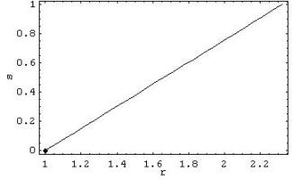
Figure 1: The statefinder parameters for NADE are plotted for the parametric values $h_{0}=1.1$, $n=0.03$, $C_{3}=0.02$, $C_{4}=0.03$, $C_{5}=0.04$ and $u=v=1.1$

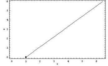
Figure 2: The statefinder parameters for HDE are plotted for the parametric values $h_{0}=0.9$, $c=0.5$, $C_{1}=0.02$, $C_{2}=0.3$,and $u=1.1$ and $v=1.2$

References

-
[1]
A. G. Riess et al. [Supernova Search Team Collaboration],
Astron. J. 116 (1998) 1009;
S. Perlmutter et al. [Supernova Cosmology Project Collaboration], Astrophys. J. 517 (1999) 565;
P. Astier et al., Astron. Astrophys. 447 (2006) 3. -
[2]
K. Abazajian et al. [SDSS Collaboration],
Astron. J. 128 (2004) 502;
K. Abazajian et al. [SDSS Collaboration], Astron. J. 129 (2005) 1755. -
[3]
D.N. Spergel et al. [WMAP Collaboration],
Astrophys. J. Suppl. 148 (2003) 175;
D.N. Spergel et al., astro-ph/0603449. -
[4]
V. Shani and A.
Starobinsky, Int. J. Mod. Phys. D 9 (2000) 373;
S. M. Carroll, Living Rev. Rel. 4 (2001) 1;
T. Padmanabhan, Phys. Rept. 380 (2003) 253;
E.J. Copeland, M. Sami and S. Tsujikawa, Int. J. Mod. Phys. D 15 (2006) 1753;
V. Sahni and A.A. Starobinsky, Int. J. Mod. Phys. D 15 (2006) 2105;
J.A. Frieman, M.S. Turner and D. Huterer, Ann. Rev. Astron. Astrophys. 46 (2008) 385;
R. Durrer and R. Maartens, arXiv:0811.4132 [astro-ph]. -
[5]
B. Ratra and P.J.E. Peebles, Phys. Rev. D 37 (1988) 3406;
C. Wetterich, Nucl. Phys. B 302 (1988) 668; R.R. Caldwell, R. Dave and P.J. Steinhardt, Phys. Rev. Lett. 80 (1998) 1582;
I. Zlatev, L.M. Wang and P.J. Steinhardt, Phys. Rev. Lett. 82 (1999) 896. - [6] C. Armendariz-Picon, V.F. Mukhanov and P.J. Steinhardt, Phys. Rev. Lett. 85 (2000) 4438.
-
[7]
A. Sen, JHEP 0207 (2002) 065;
T. Padmanabhan, Phys. Rev. D 66 (2002) 021301;
M.R. Setare, J. Sadeghi and A.R. Amani, Phys. Lett. B 673 (2009) 241. -
[8]
R. R. Caldwell, Phys. Lett. B 545 (2002) 23;
S. Nojiri and S.D. Odintsov, Phys. Lett. B 562 (2003) 147;
Y.H. Wei and Y. Tian, Class. Quant. Grav. 21 (2004) 5347;
V.K. Onemli and R.P. Woodard, Phys. Rev. D 70 (2004) 107301;
M. R. Setare, Eur. Phys. J. C 50 (2007) 991. -
[9]
B. Feng, X.L. Wang and X.M. Zhang, Phys. Lett. B 607 (2005) 35;
Z.K. Guo, Y.S. Piao, X.M. Zhang and Y.Z. Zhang, Phys. Lett. B 608 (2005) 177;
A. Anisimov, E. Babichev and A. Vikman, JCAP 0506 (2005) 006;
Y-F. Cai, H. Li, Y.S. Piao and X. Zhang, Phys. Lett. B 646 (2007) 141;
M.R. Setare, J. Sadeghi, and A.R. Amani, Phys. Lett. B 660 (2008) 299;
J. Sadeghi, M.R. Setare , A. Banijamali and F. Milani, Phys. Lett. B 662 (2008) 92;
M.R. Setare and E.N. Saridakis, Phys. Lett. B 668 (2008) 177;
M.R. Setare and E.N. Saridakis, arXiv:0807.3807 [hep-th];
M.R. Setare and E.N. Saridakis, JCAP 09 (2008) 026. - [10] E. Witten, hep-ph/0002297.
- [11] A.G. Cohen, D.B. Kaplan and A.E. Nelson, Phys. Rev. Lett. 82 (1999) 4971.
-
[12]
G. ’t Hooft, gr-qc/9310026;
L. Susskind, J. Math. Phys. 36 (1995) 6377;
P. Horava and D. Minic, Phys. Rev. Lett. 85 (2000) 1610;
S.D. Thomas, Phys. Rev. Lett. 89 (2002) 081301. - [13] S.D.H. Hsu, Phys. Lett. B 594 (2004) 13.
-
[14]
M. Li, Phys. Lett. B 603 (2004) 1;
M. Jamil and M.U. Farooq, JCAP 1003 (2010) 001;
M. Jamil and M.U. Farooq, Int. J. Theor. Phys. 49 (2010) 42;
M.R. Setare and M. Jamil, JCAP 1002 (2010) 010;
M. Jamil, E.N. Saridakis and M.R. Setare, Phys. Lett. B 679 (2009) 172;
M. Jamil, M.U. Farooq and M.A. Rashid, Eur. Phys. J. C 61 (2009) 471;
M. Jamil and E.N. Saridakis, JCAP 07 (2010) 028. - [15] Q.G. Huang and Y.G. Gong, JCAP 0408 (2004) 006.
- [16] Z. Chang, F.Q. Wu and X. Zhang, Phys. Lett. B 633 (2006) 14.
- [17] X. Zhang and F.Q. Wu, Phys. Rev. D 72 (2005) 043524.
-
[18]
Q. Wu, Y. Gong, A. Wang and J.S. Alcaniz,
Phys. Lett. B 659 (2008) 34;
Y.Z. Ma and Y. Gong, Eur. Phys. J. C 60 (2009) 303. -
[19]
K. Enqvist, S. Hannestad and M.S. Sloth, JCAP 0502 (2005) 004;
J. Shen, B. Wang, E. Abdalla and R.K. Su, Phys. Lett. B 609 (2005) 200;
H.C. Kao, W.L. Lee and F.L. Lin, Phys. Rev. D 71 (2005) 123518. -
[20]
R.C. Myers and M.J. Perry, Annals Phys. 172 (1986) 304;
P. Kanti and K. Tamvakis, Phys. Rev. D 68 (2003) 024014. - [21] Q.G. Huang and M. Li, JCAP 0408 (2004) 013.
-
[22]
M. Ito, Europhys. Lett. 71 (2005) 712;
K. Enqvist and M.S. Sloth, Phys. Rev. Lett. 93 (2004) 221302;
Q.G. Huang and M. Li, JCAP 0503 (2005) 001;
D. Pavon and W. Zimdahl, Phys. Lett. B 628 (2005) 206;
B. Wang, Y. Gong and E. Abdalla, Phys. Lett. B 624 (2005) 141;
H. Kim, H.W. Lee and Y.S. Myung, Phys. Lett. B 632 (2006) 605;
S. Nojiri and S.D. Odintsov, Gen. Rel. Grav. 38 (2006) 1285;
E. Elizalde, S. Nojiri, S.D. Odintsov and P. Wang, Phys. Rev. D 71 (2005) 103504;
B. Hu and Y. Ling, Phys. Rev. D 73 (2006) 123510;
H. Li, Z.K. Guo and Y.Z. Zhang, Int. J. Mod. Phys. D 15 (2006) 869;
M.R. Setare, Phys. Lett. B 642 (2006) 1;
M.R. Setare, Phys. Lett. B 642 (2006) 421;
E.N. Saridakis, Phys. Lett. B 660 (2008) 138;
E.N. Saridakis, JCAP 0804 (2008) 020;
E.N. Saridakis, Phys. Lett. B 661 (2008) 335. -
[23]
L. Amendola, Phys. Rev. D 62 (2000) 043511;
D. Comelli, M. Pietroni and A. Riotto, Phys. Lett. B 571 (2003) 115;
M.R. Setare, JCAP 0701 (2007) 023;
M.R. Setare and E.N. Saridakis, Phys. Lett. B 670 (2008) 1. - [24] R. G. Cai, Phys. Lett. B 657 (2007) 228.
- [25] H. Wei and R.G. Cai, Phys. Lett. B 660 (2008) 113.
- [26] H. Wei and R.G. Cai, Eur. Phys. J. C 59 (2009) 99.
-
[27]
H. Wei and R.G. Cai, Phys. Lett. B 663 (2008) 1;
Y.W. Kim, H.W. Lee, Y.S. Myung, M-I. Park, Mod. Phys. Lett. A 23 (2008) 3049;
Y. Zhang, H. Li, X. Wu, H. Wei and R-G. Cai arXiv:0708.1214 [astro-ph];
K.Y. Kim, H.W. Lee and Y.S. Myung, Phys. Lett. B 660 (2008) 118;
X. Wu, Y. Zhang, H. Li, R-G. Cai, Z-H. Zhu, arXiv:0708.0349 [astro-ph];
I.P. Neupane, Phys. Lett. B 673 (2009) 111;
J. Zhang, X. Zhang and H. Liu, Eur. Phys. J. C 54 (2008) 303;
J .P Wu, D. Z. Ma and Y. Ling, Phys. Lett. B 663 (2008) 152. -
[28]
S. Nojiri and S.D. Odintsov, Int. J. Geom. Meth. Mod. Phys. 4
(2007) 115;
S. Capozziello and M. Francaviglia, Gen. Relativ. Gravit. 40 (2008) 357. - [29] L. Amendola and S. Tsujikawa, Phys. Lett. B 660 (2008) 125.
- [30] M.C.B. Abdalla, S. Nojiri and S.D. Odintsov, Class. Quant. Grav. 22 (2005) L35.
-
[31]
V. Sahni and Y. Shtanov, JCAP 0311 (2003) 014;
V. Sahni, astro-ph/0502032;
K. Bamba, C-Q. Geng, S. Nojiri and S.D. Odintsov, arXiv:0810.4296 [hep-th]. - [32] U. Alam, V. Sahni, T.D. Saini and A.A. Starobinsky, Mon. Not. Roy. Astron. Soc. 354 (2004) 275.
- [33] A.C.C. Guimar es and J.A.S. Lima, arXiv:1005.2986v2 [astro-ph.CO].
- [34] M.R. Setare, Int. J. Mod. Phys. D 17 (2008) 2219.
- [35] M.R. Setare, Astrophys. Space Sci. 326 (2010) 27.
- [36] S.A. Appleby, R.A. Battye and A.A. Starobinsky, JCAP 1006 (2010) 005.
-
[37]
S. Nojiri and S.D. Odintsov, Phys. Rev. D 68 (2003) 123512;
S. Nojiri and S.D. Odintsov, Gen. Rel. Gravit. 36 (2004) 1765. - [38] V. Faraoni, Phys. Rev. D 74 (2006) 104017.
-
[39]
S. Capozziello, S. Carloni and A. Troisi,
astro-ph/0303041;
S.M. Carroll, V. Duvvuri, M. Trodden and M.S. Turner, Phys. Rev. D 70 (2004) 043528;
X. Meng and P. Wang, Class. Quant. Grav. 20 (2003) 4949;
S.M. Carroll, A. De Felice, V. Duvvuri, D.A. Easson, M. Trodden, and M.S. Turner, Phys. Rev. D 71 (2005) 063513. - [40] R. Reyes et al, Nature, 464 (2010) 256.
- [41] V. Sahni, T.D. Saini, A.A. Strarobinsky and U. Alam, JETP Lett. 77 (2003) 201.
- [42] U. Alam, V. Sahni, T.D. Saini and A.A. Starobinsky, Mon. Not. Roy. Astron. Soc. 344 (2003) 1057.
- [43] U. Debnath, Class. Quant. Grav. 25 (2008) 205019.
- [44] X. Zhang, Int. J. Mod. Phys. D 14 (2005) 1597.
- [45] H. Wei and R.G. Cai, Phys. Lett. B 655 (2007) 1.
- [46] X. Zhang, Phys. Lett. B 611 (2005) 1.
- [47] Z.G. Huang, X.M. Song, H.Q. Lu and W. Fang, Astrophys. Space Sci. 315 (2008) 175.
- [48] W. Zhao, Int. J. Mod. Phys. D 17 (2008) 1245.
- [49] M. Hu and X.H. Meng, Phys. Lett. B 635 (2006) 186.
- [50] W. Zimdahl and D. Pavon, Gen. Rel. Grav. 36 (2004) 1483.
- [51] Y. Shao and Y. Gui, Mod. Phys. Lett. A 23 (2008) 65.
- [52] W. Chakraborty and U. Debnath, Mod. Phys. Lett. A 22 (2007) 1805.
- [53] S. Li, H-R. Yu and T-J. Zhang, 1002.3867 [astro-ph.CO].
- [54] M. Jamil and U. Debnath, arXiv:0909.3689 [gr-qc].