Spacial and temporal dynamics of the volume fraction of the colloidal particles inside a drying sessile drop

Abstract

Using lubrication theory, drying processes of sessile colloidal droplets on a solid substrate are studied. A simple model is proposed to describe temporal dynamics both the shape of the drop and the volume fraction of the colloidal particles inside the drop. The concentration dependence of the viscosity is taken into account. It is shown that the final shapes of the drops depend on both the initial volume fraction of the colloidal particles and the capillary number. The results of our simulations are in a reasonable agreement with the published experimental data. The computations for the drops of aqueous solution of human serum albumin (HSA) are presented.

1 Introduction

The patterns observed after the complete desiccation of sessile drop of a biological fluid such as serum, cerebrospinal fluid, urine etc. attract the attention of the researchers at least since the 1950s Sole1954 ; Koch1954 ; Koch1956 . In the last few decades, the interest to the pattern formation in drying drops of the biological fluids growths stably in the contexts of numerous applications (e.g. medical tests Savina1999 ; Shabalin2001 ; Rapis2002 , drug screening Takhistov2002 , biostabilization Ragoonanan2008 etc). State of the art can be found in Tarasevich2004 ; Yakhno2009 .

More extensive investigations are performed in the adjacent field that is evaporative selfassembly of nano- and microparticles from an evaporating sessile drop. This process is known as an important surface-patterning technique which has potential application in optical, microelectronic, and sensory devices.

Several models of deposit formation in drying drops were proposed during last few years Parisse1996 ; Deegan2000 ; Fischer2002 ; Popov2005 ; Widjaja2008 ; Attinger2009 ; Zheng2009 ; Witten2009 ; Sefiane2009Langmuir ; Petsi2010 ; Kistovich2010 . Mostly, the particles were considered as noninteracting and the formed deposit hasn’t any effect on both evaporation and bulk flows. It is rather clear that these assumptions restrict the possible application of the proposed models to the particular kind of the solutes.

One have to utilize quite different approach, if a phase transition (sol to gel or sol to glass) occurs as a result of increasing the particle volume fraction due to the solvent loss and internal flows. The models interpreting deposit as impermeable both for hydrodynamical flows and evaporation were proposed recently Okuzono2009 ; Vodolazskaya2010 .

Thus, the work Okuzono2009 is devoted to study the drying processes of polymer solutions on a solid substrate enclosed by bank. Drying process is studied in the slow limit of the solvent evaporation. The model is based on mass conservation. The master equation is a diffusion-advection equation.

Processes inside desiccated sessile drop depend on various physical and chemical conditions such as the wetting property of the substrate and surface roughness, the particle size, the size distribution, the particle concentration in the droplet, the relative humidity of the evaporation environment, ionic strength, and pH.

If the initial volume fraction of the colloidal particles inside a drop is large enough, the contact line does not recede during the evaporation process, depinning and stick-slip motion is not observed. In particular, it was shown that desiccation of the colloidal suspensions considerably depends on the competition between evaporation and gelation Pauchard1999 . Classification of the possible regimes of the desiccation can be done in terms of the desiccation time $t_{\text{d}}$ and the gelation time $t_{\text{g}}$. Our investigation is restricted to the case when the desiccation time is very short compared with gelation time $t_{\text{d}}\ll t_{\text{g}}$. In this case a solid gelled or glassed foot builds up near the drop edge, while the central part remains fluid.

For this particular situation, the desiccation process can be divided into several stages:

Pregelation stage.

The early time regime where a gel-like phase does not appear and the whole volume of the drop is liquid. During this stage, the solvent evaporates, the colloidal particles are transferred by the outward flow to the drop edge and accumulate near the contact line.

Gelation stage.

The concentration of colloidal particles at the contact line reaches the gelation concentration $C_{\text{g}}$ above which a gel or glass phase appears. The gel (glass) phase region begins to develop from the edge and the phase front monotonically move from edge to center.

Postgelation stage.

The drop is solid-like, the loss of solvent confined among the colloidal particles evaporates very slowly, the cracks appeare all around the drop.

The first stage was investigated in detail in the series of works Tarasevich2007TP ; Tarasevich2007epje ; Tarasevich2010TP , as well as in Okuzono2009 . In the present article, we focus efforts on the second stage only.

The construction of this paper is as follows. In Section 2, we describe our model. In Section 3 the obtained results are discussed. Finally, we summarize our results and conclude this paper.

2 Model and assumptions

2.1 Problem Formulation

We will consider axisymmetric sessile drop of a colloidal solution. We assume that volume fraction of the dispersed particles is high enough to ensure strong adhesion of the drop, in such a way the contact line of a drop is pinned during the drying process. When the environmental conditions are homogeneous and isotropic, the flow field inside the drop has to be axisymmetric, too.

We will use cylindrical coordinates $(r,z,\phi)$, because they are natural for the geometry of sessile drops. The origin is chosen in the center of the drop on the substrate. The coordinate $z$ is normal to the substrate, and the substrate is described by $z=0$, with $z$ being positive on the droplet side of the space. The coordinate $r$ is the polar radius. Due to the axial symmetry of the problem and our choice of the coordinates, no quantity depends on the azimuthal angle. In this case flow field inside a drop has only two components:

$$\mathbf{v}(r,z,t)=u(r,z,t){\mathbf{n}_{r}}+w(r,z,t){\mathbf{n}_{z}}.$$

The density of particles is supposed to be equal to the density of pure solvent. This density, $\rho$, is presumed to be constant during desiccation. These assumptions are quite reasonable for the biological fluids.

Moreover, we suppose that diffusion transfer is negligibly compared with advection.

Only small drops are of the practical interest, thus, we assume that the droplet is sufficiently small so that the surface tension is dominant, and the gravitational effects can be neglected. The temperature gradient along the interface of the droplet is assumed to be significantly weak so that thermal Marangoni flow is not induced. Moreover, we will neglect the concentration dependence of the surface tension $\sigma$ (i.e. the concentration Marangoni flow is absent, too).

The evaporation process can be considered as quasi-steady and we will suppose that system is steady at every moment.

Above assumptions allow us to apply the lubrication approximation Burelbach1988 to the drop. This approach was used in Fischer2002 ; Okuzono2009 , too. By applying the lubrication approximation to the continuity and Navier-Stokes equations, fluid flow is governed by

$$-\frac{\partial p}{\partial r}+\eta\frac{{{\partial^{2}}u}}{{\partial{z^{2}}}} =0,$$

$$-\frac{\partial p}{{\partial z}} =0,$$

$$\frac{1}{r}\frac{{\partial(ru)}}{\partial r}+\frac{{\partial w}}{{\partial z}} =0,$$

where $p$ is the pressure and $\eta$ is the viscosity.

The boundary conditions should be written as

$${\left.p\right|_{z=h}} =-\frac{\sigma}{r}\frac{\partial}{\partial r}\left({r\frac{\partial h}{\partial r}}\right), \quad{\left.{\frac{{\partial u}}{{\partial z}}}\right|_{z=h}} =0,$$ (1)

$${\left.u\right|_{z=0}} =0, \quad{\left.w\right|_{z=0}} =0,$$

where $h(r,t)$ is the droplet height profile.

In the lubrication approximation, the velocity field can be written as a function of drop profile $h(r,t)$

$$u =-\frac{\sigma}{\eta}\frac{\partial}{\partial r}\left({\frac{1}{r}\frac{\partial}{\partial r}\left({r\frac{\partial h}{\partial r}}\right)}\right)\left({\frac{{{z^{2}}}}{2}-hz}\right),$$ (2)

$$w =\frac{\sigma}{r}\frac{\partial}{\partial r}\left({\frac{r}{\eta}\frac{\partial}{\partial r}\left({\frac{1}{r}\frac{\partial}{\partial r}\left({r\frac{\partial h}{\partial r}}\right)}\right)\left({\frac{{{z^{3}}}}{6}-h\frac{{{z^{2}}}}{2}}\right)}\right).$$

The height-averaged radial velocity calculated using (2) is given by

$$\left\langle u\right\rangle=\frac{1}{h}\int\limits_{0}^{h}{u\,dz}=\frac{{{h^{2}}}}{3}\frac{\sigma}{\eta}\frac{\partial}{\partial r}\left({\frac{1}{r}\frac{\partial}{\partial r}\left({r\frac{\partial h}{\partial r}}\right)}\right).$$ (3)

From the conservation of solvent, the height-evolution equation is given by

$$\frac{\partial h}{{\partial t}}=-\frac{1}{r}\frac{{\partial(rh\left\langle u\right\rangle)}}{\partial r}-\frac{J}{\rho},$$ (4)

where $J(r,t)$ is the spatial and time-dependent solvent mass flux at the air-liquid interface.

From the conservation of solute, the height-averaged solute concentration $\langle C(r,t)\rangle$ is given by

$$\frac{{\partial(h\langle C\rangle)}}{{\partial t}}=-\frac{1}{r}\frac{\partial}{\partial r}\left({rh\langle C\rangle\langle u\rangle}\right).$$ (5)

If a drop is small and surface tension dominates over gravity, the shape of the drop is close to an equilibrium shape, i.e. spherical cap. Without considerable loss of precision we can suppose that a drop has more simple shape as a paraboloid of revolution. Nevertheless, the real shape of the drop profile near the contact line is questionable. Note that widely used assumption about spherical cap shape leads to singularities both in evaporation flux and flow rate Deegan2000 . Particularly, the precursor film of a wetting drop was discussed in Takhistov2002 .

The subject of our investigation is only the second stage of drying process when colloidal particles are accumulated at the edge of the droplet. Hence, we can suppose that drop edge has very small thickness.

Taking into account pinning and the axial symmetry of the problem, the boundary and initial conditions for the set of equations (4), (5) can be written as

$${\left.h\right|_{t=0}} =h_{\text{f}}+{h_{0}}\left({1-{{\left({\frac{r}{R}}\right)}^{2}}}\right),$$ (6)

$${\left.{\langle u\rangle}\right|_{r=0}} ={\left.{\langle u\rangle}\right|_{r=R}}=0,$$

$${\left.{\frac{\partial h}{\partial r}}\right|_{r=0}} =0,$$

$${\left.h\right|_{r=R}} =h_{\text{f}},$$

$$\langle C(r,0)\rangle =f(r),$$

$${\left.{\frac{{\partial\langle C\rangle}}{\partial r}}\right|_{r=0}} =0,$$

where ${f(r)}$ is the initial concentration of the colloidal particle, $h_{0}+h_{\text{f}}$ is the initial height of the drop apex, $h_{\text{f}}$ is the initial height of the drop edge ($h_{\text{f}}\ll h_{0}$).

To nondimensionalize the equations, the vertical coordinate was scaled by the initial droplet height ${h_{0}}$, the radial coordinate was scaled by the drop radius $R$, the velocities were scaled by the characteristic viscous velocity ${u_{c}}=\frac{{{\eta_{0}}}}{{\rho{h_{0}}}}$, where $\eta_{0}$ is the viscosity of pure solvent. Time was scaled by $\frac{R}{{{u_{c}}}}$, vapor flux was scaled by ${J_{c}}=\frac{{k\Delta T}}{{L{h_{0}}}}$, where $k$ is the thermal conductivity of the liquid, $\Delta T$ is the temperature difference between the substrate and saturation temperatures, $L$ is the heat of vaporization. The height-averaged concentration was scaled by gelation concentration $C_{\text{g}}$.

Upon scaling, the evaporation number, $\mathrm{E}=\frac{{k\Delta T}}{{\varepsilon{\eta_{0}}L}}$, and the capillary number, $\mathrm{Ca}=\frac{{{\eta_{0}}{u_{c}}}}{{{\varepsilon^{3}}\sigma}}$, where $\varepsilon=\frac{{{h_{0}}}}{R}$, appear as the dimensionless parameters.

In the dimensionless form, dynamics of the drop profile and the concentration of the colloidal particles are governed by

$$\frac{\partial h}{{\partial t}}=-\frac{1}{r}\frac{{\partial(rh\left\langle u\right\rangle)}}{\partial r}-J\mathrm{E},$$ (7)

$$\frac{{\partial(h\langle C\rangle)}}{{\partial t}}=-\frac{1}{r}\frac{\partial}{\partial r}\left({rh\langle C\rangle\langle u\rangle}\right),$$ (8)

where

$$\left\langle u\right\rangle=\frac{1}{\mathrm{3Ca}}\frac{h^{2}}{\eta}\frac{\partial}{\partial r}\left({\frac{1}{r}\frac{\partial}{\partial r}\left({r\frac{\partial h}{\partial r}}\right)}\right).$$ (9)

To simplify notation, we don’t use any special symbols for the dimensionless quantities.

In our consideration, we take into account concentration dependence of solvent viscosity $\eta(r,t)$. Thus, viscosity is not a constant but varies in space and time.

The master equations (7) and (8) may be reorganized and rewritten using the matrix notation

$$\frac{\partial\mathbf{F}}{\partial t}+\langle u\rangle\frac{\partial\mathbf{F}}{\partial r}=\mathbf{f},$$ (10)

$$\mathbf{F}=\begin{pmatrix}h\\ \langle C\rangle\end{pmatrix},$$ (11)

$$\mathbf{f}=\begin{pmatrix}-\dfrac{h}{r}\dfrac{\partial}{\partial r}(r\langle u\rangle)-\mathrm{E}J\\ \mathrm{E}\dfrac{\langle C\rangle J}{h}\end{pmatrix}.$$ (12)

In the framework of the lubrication approximation, the evaporative mass flux must be equal to zero at the contact line. To our best knowledge the experimental data on evaporative flux over the free surface of a colloidal droplet with moving phase front inside it are not published yet. We will exploit the mass flux of evaporating liquid derived from the heat transfer analysis Anderson1995

$$J(r,t)=\frac{1}{\kappa+h(r,t)},$$

where $\kappa$ is a dimensionless nonequilibrium parameter. $\kappa\to\infty$ for nonvolatile substances and $\kappa\to 0$ for high volatile liquids. A conjecture that colloidal particles accumulated at the edge of the droplet must hinder the evaporation at the contact line was proposed by Fischer Fischer2002 . The author introduced an additional factor in evaporative flux so that the flux decreases exponentially near the contact line. We suppose that the density of vapor vanishes not at the edge of a drop but at the sol-gel phase boundary. In the other words, the vapor flux has to be zero if the concentration of the colloidal particles reaches a critical value ($C=1$), which corresponds to a phase transition (sol to gel or sol to glass):

$$J(r,t)=\frac{1-\langle C\rangle^{2}(r,t)}{\kappa+h(r,t)}.$$ (13)

We should notice that the results of computations depend drastically on particular form of the evaporation flux. Our choice (13) provides linear decreasing with time of the drop mass Deegan2000 ; Annarelli2001 and the reasonable dynamics of drop shape (see Section 3).

2.2 Parameters of the model

The computations were performed with $\mathrm{Ca}=0.01,0.1,1,10$ and $\mathrm{E}=0.01,0.1,1$, as well as with the $\mathrm{Ca}$ and $\mathrm{E}$, which correspond to the drops of biological fluid used in the medical tests. In the medical tests, the typical drop volume varies between 10 and 20 $\mu$l with diameter 5–7 mm (Shabalin2001, , p. 100). It means that typical drop height is $h_{0}\approx 1$ mm. In general, the drop height should be lower, since we consider only the second stage of desiccation, when the volume fraction of the colloidal particles reaches the critical value of $\Phi_{\text{g}}$ near the drop edge. Nevertheless, the experiments Yakhno2004 as well as the simulations Okuzono2009 ; Tarasevich2010TP show that the first stage lasts only about 10 % of desiccation time. Taking into account linear decreasing of the drop height, we can ignore the height change. We take the middle value $R=3$ mm as the typical radius, so $\varepsilon\approx 0.33$. Assuming $\rho=10^{3}$ kg/m³, $\eta_{0}=10^{-3}$ Pa$\cdot$sec, and $\sigma=73\cdot 10^{-3}$ N/m, the characteristic viscous velocity will be $u_{\text{c}}=10^{-3}$ m/sec. In this case the capillary number will be $\mathrm{Ca}\approx 4\cdot 10^{-4}$. It should be noted that $\varepsilon^{2}\approx 0.1$, hence the lubrication approximation is still valid. The rest of the quantities of use are $k=0.6$  W/(m K), $\Delta T=80$ K$,L=2.25\cdot 10^{6}$ J/kg, hence $\mathrm{E}\approx 3\cdot 10^{-2}$.

The experimental data of solution viscosities of HSA for concentrations ranges from $8.2$ up to $369$ kg/m³ at pH$=7.0$ and temperature $20^{\circ}$ C were taken from Monkos2004 . The volume fraction of colloidal particles can be calculated as

$$\Phi=\frac{VC}{M_{\text{h}}},$$

where $V=\frac{4}{3}\pi pb^{3}$ is the hydrodynamic volume of one dissolved protein ($a$ and $b$ are the effective semi-axes of hydrated HSA and $p$ is the axial ratio), $M_{\text{h}}=91.675$ kDa is the molecular mass of the dissolved protein Monkos2004 .

Taking into account the data published in Monkos2005 , $a=8.2$ nm, $b=2.1$ nm, $p=3.95$, we can get the relation $\Phi=10^{-3}C$. Then the volume fraction was divided by $\Phi_{\text{g}}=0.5$. Nondimensional data were fitted by Mooney’s formula using least square method

$$\eta=\eta_{0}\exp\left(\frac{S\Phi}{1-K\Phi}\right),$$ (14)

where $\eta_{0}$ is the viscosity of pure solvent (see fig. 1).

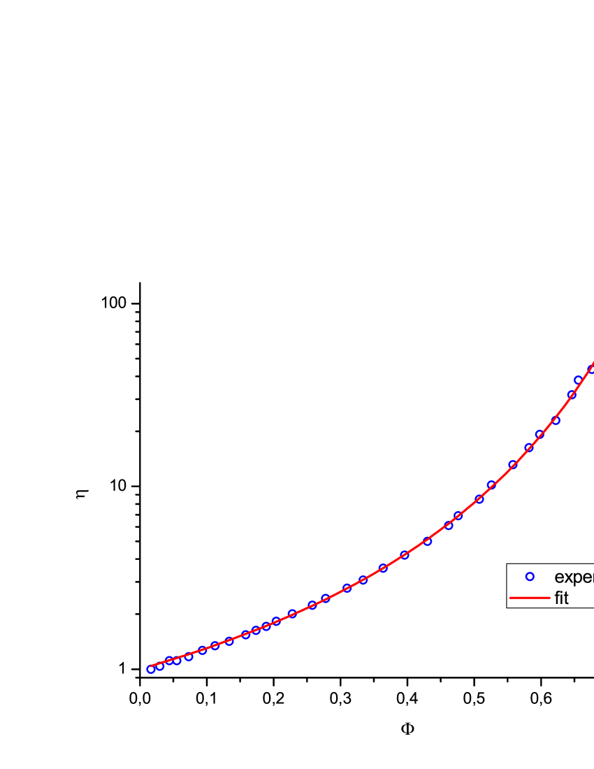
Figure 1: Nondimensional viscosity vs. normalized volume fraction: experiment Monkos2004 and fit by Mooney (14).

For the normalized by $\Phi_{\text{g}}$ volume fraction and nondimensional viscosity, the fitting parameters are $S=2.42\pm 0.07$ and $K=0.84\pm 0.02$.

One can calculate the density of the hydrated protein $\rho\approx 993$ kg/m³, hence our assumption (Section 2.1) about equality of the solute and solvent densities holds for aqueous solution.

The initial concentration can be written as

$$f(r)=2-\langle C_{0}\rangle+2\frac{\langle C_{0}\rangle-1}{1+\exp(w(r-1))},$$

where $w$ is an adjustable constant, it is related to the length over which the concentration of colloidal particles increases rapidly. $w=10$ in all computation presented in this article. This choice gives us a good agreement with the calculated distribution at the end of the first stage of desiccation Tarasevich2007TP ; Tarasevich2007epje ; Tarasevich2010TP . Notice, that $f(0)\approx\langle C_{0}\rangle$ and $f(1)=1$.

Computations in Tarasevich2010TP demonstrate, that at the begin of the second stage, the concentration in the drop center is approximately equal to the initial concentration. Notice, that in Okuzono2009 the concentration in the drop center growths at the rate one and a half times. This fact is the natural consequence of utilized uniform vapor flux over the free surface.

$\kappa=0.01$ and $h_{\text{f}}=0.01$ in all presented simulations. Our computations say that the results are almost insensitive to $h_{\text{f}}$, if the relation $h_{\text{f}}\ll h_{0}$ is valid.

3 Results

The results of our simulations are presented in figs. 2, 3, 4, 5, 6, 7. $t_{\text{max}}$ occurring in the captions relates to the time of the whole drop bulk becoming solid-like and the drop height almost not decreasing.

Mass of the drop decreases linearly until almost all solvent lost from the drop, then it stays nearly constant (Fig. 2). This behavior agrees with the published experimental results (see e.g. Deegan2000 ; Annarelli2001 ) and demonstrates that the proposed evaporation flux (13) is rather adequate. In our simulations, difference between mass of the completely dried drop and the initial total mass of the colloidal particles does not exceed 1.5 %. This fact confirms that computations are quite correct.

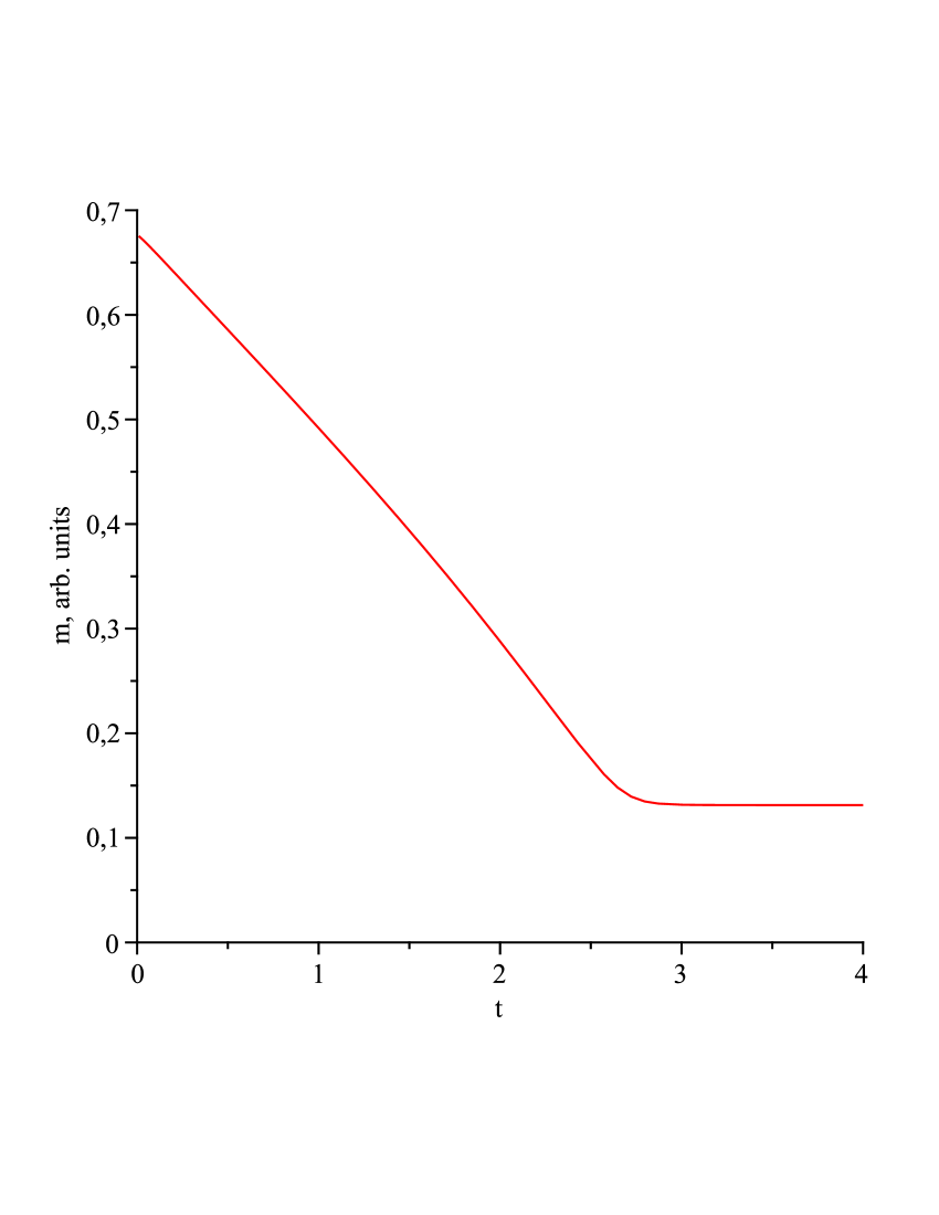
Figure 2: Temporal dynamics of mass, with $\mathrm{Ca}=0.1$, $\mathrm{E}=0.1$, $\Phi_{0}=0.2$.

Drop height decreases approximately in linearly manner until almost all solvent evaporates from the drop, then it remains unchanged (Fig. 3). This behavior is typical just for the case when $t_{\text{d}}\ll t_{\text{g}}$ Pauchard1999 , which is the subject of our investigations.

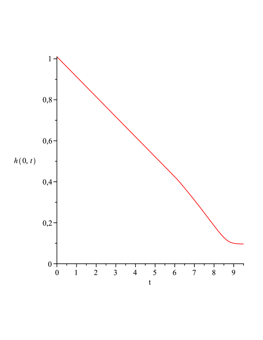
Figure 3: Temporal height dynamics, with $\mathrm{Ca}=4\cdot 10^{-4}$, $\mathrm{E}=0.03$, $\Phi_{0}=0.2$.

We have investigated the effect of initial volume fraction of the colloidal particles inside the drop on time evolution of the droplet height profile as well as distribution of the colloidal particles (Fig. 4). If the initial volume fraction is low there will be visible roller around the edge of dried sample. If the initial volume fraction has an intermediate value the final shape of the sample looks like a pancake, with a depressed central zone. Indeed, if the initial volume fraction is close to the value $\Phi_{\text{g}}$ the drop shape varies very low. Notice that profile evolution dynamics during early time is very similar to the dynamics of the constant base model proposed in Parisse1996 .

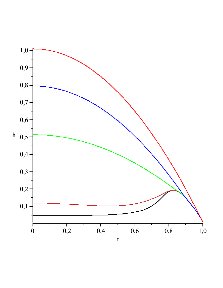
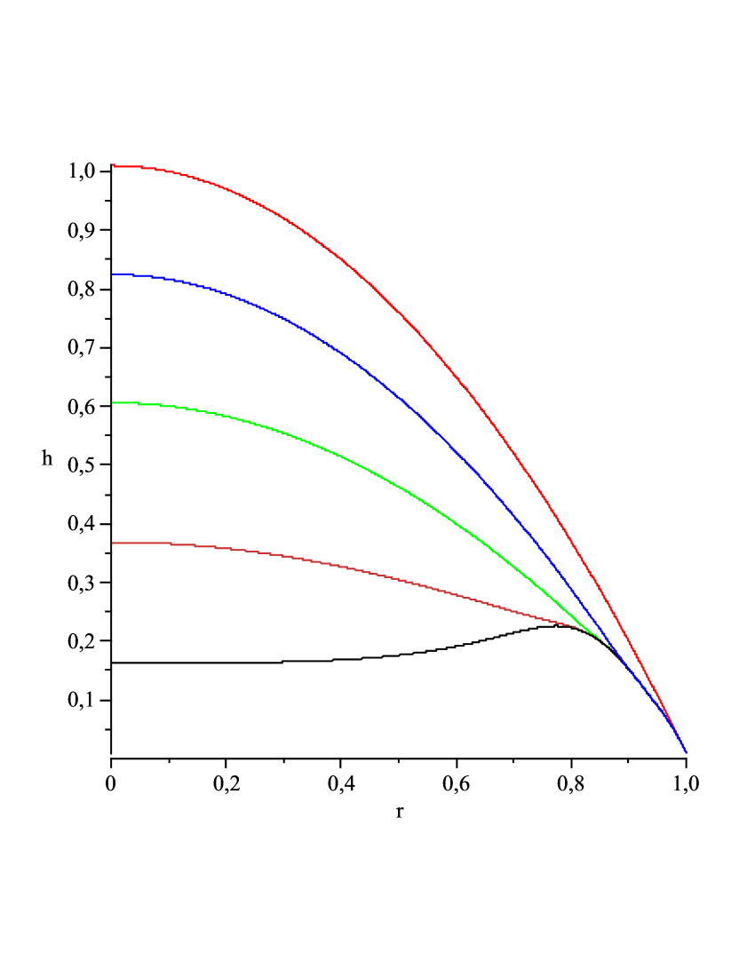
a) b) c)

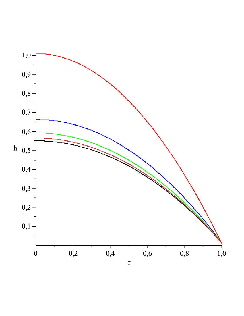
Figure 4: (Color online) Time evolution of the droplet height profile for $t/t_{\text{max}}=0,0.25,0.5,0.75,1$, with $\mathrm{Ca}=0.1$, $\mathrm{E}=0.1$. a) $\Phi_{0}=0.1$, b) $\Phi_{0}=0.25$, c) $\Phi_{0}=0.4$.

Fig. 5 shows our results obtained for fixed initial volume fraction and evaporation number and with different values of capillary number. If capillary number is small (i.e. surface-tension forces dominate viscous forces) early time evolution of the droplet height profile is similar to constant base model Parisse1996 . If the capillary number is large, then viscous forces will dominate surface tension forces. In this case profile dynamics corresponds to constant angle model Parisse1996 . It looks like if the capillary number is intermediate, then the evolution of profile is closer to the predictions of model proposed by Popov Popov2005 . Thus, the known models are suitable and correct for different particular cases and can be reproduced within our model.

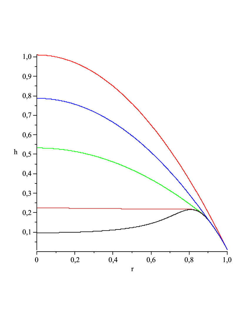
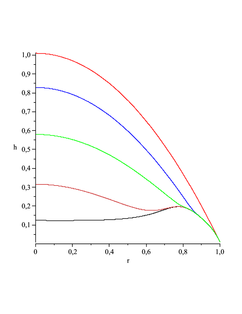
a) b) c)

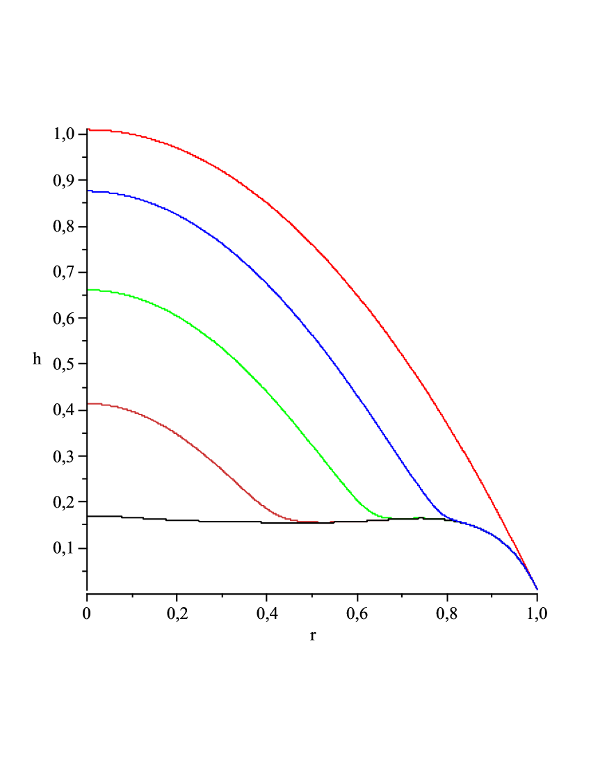
Figure 5: (Color online) Time evolution of the droplet height profile for $t/t_{\text{max}}=0,0.25,0.5,0.75,1$, with $\Phi_{0}=0.2$, $\mathrm{E}=0.1$. a) $\mathrm{Ca}=0.01$, b) $\mathrm{Ca}=1$, c) $\mathrm{Ca}=10$.

Evolution of the colloidal particle distribution is depicted in Fig. 6. This result is in qualitative agreement with Okuzono2009 .

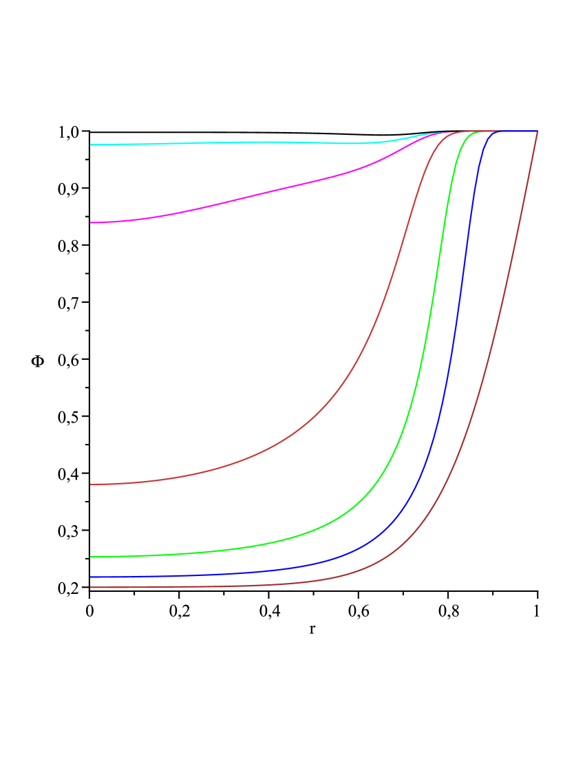
Figure 6: (Color online) Evolution of the particle volume fraction for $t/t_{\text{max}}=0,0.25,0.5,0.75,0.9,0.95,1$, with $\mathrm{Ca}=0.1$, $\mathrm{E}=0.1$, $\Phi_{0}=0.2$.

Moreover, some computations have been performed for the parameters which are close to the values for samples used in the medical tests. Time evolution of the droplet height profile is presented in Fig. 7. Notice that final shape of the drop is a flat pancake, with a depressed central zone (Fig.7) and looks like the real sample (Fig. 8).

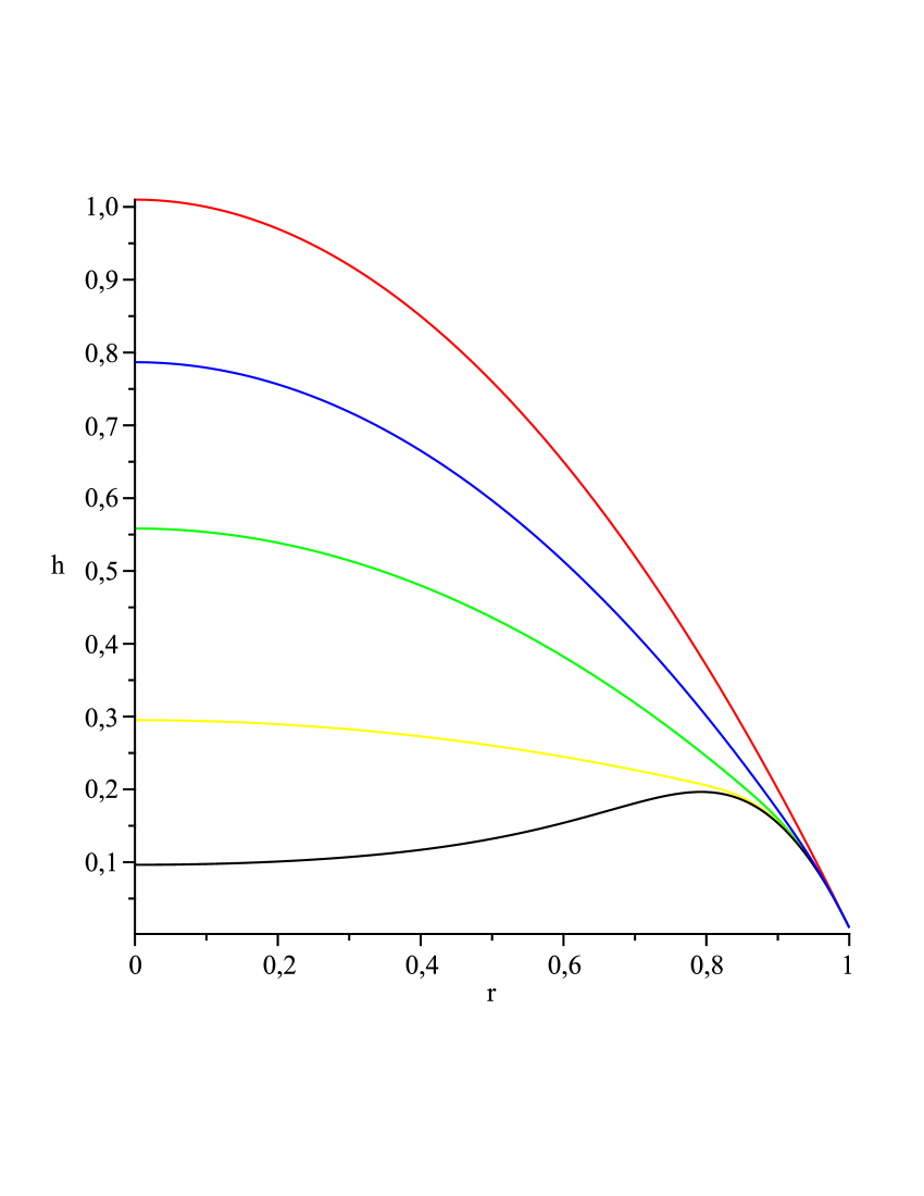
Figure 7: (Color online) Time evolution of the droplet height profile for $t/t_{\text{max}}=0,0.25,0.5,0.75,1$, with $\mathrm{Ca}=4\cdot 10^{-4}$, $\mathrm{E}=0.03$, $\Phi_{0}=0.2$.

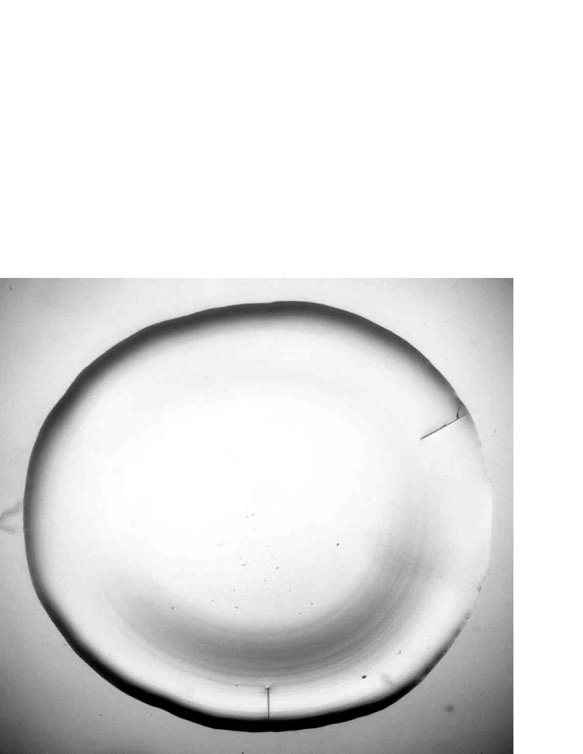
Figure 8: Sample of a drop after 16 min it was placed onto glass slide (10 w% of BSA in normal saline solution). (Courtesy T.A. Yakhno).

4 Conclusion

The main open question of our work is related to the real form of evaporation flux and adequacy of our choice (13). In our opinion, this question can be resolved only experimentally.

The biological fluids contain both colloidal particles (proteins) and the salts. Salts have rather high diffusivity, hence they cannot be described using (10). It is of interest and of value to include in the model additional spices with high diffusivity. The natural way to improve the proposed model is to supplement the set of equations (10) with additional advection-diffusion equation describing spatial and temporal dynamics of salt Tarasevich2007TP ; Tarasevich2007epje ; Tarasevich2010TP .

- (1) A. Sole, Colloid & Polymer Science 137, 15 (1954)
- (2) C. Koch, Colloid & Polymer Science 138, 81 (1954)
- (3) C. Koch, Colloid & Polymer Science 145, 7 (1956)
- (4) L.V. Savina, Crystalloscopic Structures of Blood Serum of Healthy People and Patients (Sov. Kuban, Krasnodar, 1999), in Russian
- (5) V.N. Shabalin, S.N. Shatohina, Morphology of Human Biological Fluids (Khrizostom, Moscow, 2001), in Russian
- (6) E. Rapis, Protein and Life (Self-Assembling and Symmetry of Protein Nanostructures (Philobiblion and Milta-PKPGIT, Jerusalem and Moscow, 2003), in Russian
- (7) P. Takhistov, H.C. Chang, Industrial & Engineering Chemistry Research 41(25), 6256 (2002)
- (8) V. Ragoonanan, A. Aksan, Biophysical Journal 94(6), 2212 (2008)
- (9) Y.Y. Tarasevich, Physics-Uspekhi 47(7), 717 (2004)
- (10) T.A. Yakhno, V.G. Yakhno, Technical Physics 54, 1219 (2009)
- (11) F. Parisse, C. Allain, J. Phys. II France 6(7), 1111 (1996)
- (12) R.D. Deegan, O. Bakajin, T.F. Dupont, G. Huber, S.R. Nagel, T.A. Witten, Phys. Rev. E 62(1), 756 (2000)
- (13) B.J. Fischer, Langmuir 18(1), 60 (2002)
- (14) Y.O. Popov, Phys. Rev. E 71(3), 036313 (2005)
- (15) E. Widjaja, M. Harris, AIChE J. 54(9), 2250 (2008)
- (16) R. Bhardwaj, X. Fang, D. Attinger, New Journal of Physics 11(7), 075020 (2009)
- (17) R. Zheng, The European Physical Journal E: Soft Matter and Biological Physics 29, 205 (2009)
- (18) T.A. Witten, EPL (Europhysics Letters) 86(6), 64002 (2009)
- (19) R.V. Craster, O.K. Matar, K. Sefiane, Langmuir 25(6), 3601 (2009)
- (20) A.J. Petsi, A.N. Kalarakis, V.N. Burganos, Chemical Engineering Science 65(10), 2978 (2010)
- (21) A.V. Kistovich, Y.D. Chashechkin, V.V. Shabalin, Technical Physics 55, 473 (2010)
- (22) T. Okuzono, M. Kobayashi, M. Doi, Phys. Rev. E 80(2), 021603 (2009)
- (23) I.V. Vodolazskaya, Y.Y. Tarasevich, O.P. Isakova, Nonlinear world 8(3), 142 (2010), in Russian
- (24) L. Pauchard, F. Parisse, C. Allain, Phys. Rev. E 59(3), 3737 (1999)
- (25) Y.Y. Tarasevich, D.M. Pravoslavnova, Technical Physics 52, 159 (2007)
- (26) Y.Y. Tarasevich, D.M. Pravoslavnova, Eur. Phys. J. E 22(4), 311 (2007)
- (27) Y.Y. Tarasevich, O.P. Isakova, V.V. Kondukhov, A.V. Savitskaya, Technical Physics 55, 636 (2010)
- (28) J.P. Burelbach, S.G. Bankoff, S.H. Davis, Journal of Fluid Mechanics 195, 463 (1988)
- (29) D.M. Anderson, S.H. Davis, Physics of Fluids 7(2), 248 (1995)
- (30) C.C. Annarelli, J. Fornazero, J. Bert, J. Colombani, Eur. Phys. J. E 5(5), 599 (2001)
- (31) T.A. Yakhno, V.G. Yakhno, A.G. Sanin, O.A. Sanina, A.S. Pelyushenko, Technical Physics 49, 1055 (2004)
- (32) K. Monkos, Biochimica et Biophysica Acta (BBA) - Proteins & Proteomics 1700(1), 27 (2004)
- (33) K. Monkos, Journal of Biological Physics 31, 219 (2005)