Estimating the amount of vorticity generated by cosmological perturbations in the early universe

Abstract

We estimate the amount of vorticity generated at second order in cosmological perturbation theory from the coupling between first order energy density and non-adiabatic pressure, or entropy, perturbations. Assuming power law input spectra for the source terms, and working in a radiation background, we calculate the wave number dependence of the vorticity power spectrum and its amplitude. We show that the vorticity generated by this mechanism is non-negligible on small scales, and hence should be taken into consideration in current and future CMB experiments.

I Introduction

Cosmological perturbation theory is a crucial tool for the study of the early universe. Linear theory (see, e.g. Refs. Lifshitz ; Bonnor1957 ; Tomita1967 ; Bardeen80 ; KS ; MFB ; Ruth ) allows us to model the large scale structure of the universe Tegmark:2006az and calculate the anisotropies of the cosmic microwave background (CMB) and compare them to the data from experiments, e.g. Wmap. However, with the advent of new data sets, such as those from the full seven year running of Wmap WMAP7 or those anticipated from the recently launched Planck satellite planck , which are superior in both their quality and quantity to previous ones, we are now in a position to test predictions of higher order perturbation theory against observational data. Conversely, perturbation theory beyond linear order is necessary in order to extract the maximum amount of information from these data sets, and thus utilise them to their full potential. The second order theory has been developed by several authors (see e.g. Refs. Tomita1967 ; Bruni:1996im ; Noh:2004bc ; Bartolo:2004if ; Nakamura ; MM2008 ; MW2008 ), and there have been studies of the applications of the theory ranging from calculations of the non-Gaussianity of the primordial perturbations to investigations of higher order phenomena produced by couplings between lower order perturbations.

It is well known that at linear order in perturbation theory, different types of perturbations (classified as scalar, vector and tensor perturbations, according to their transformation behaviour on three dimensional hypersurfaces) decouple KS . However, at second order (see, e.g. Ref. MW2008 and references therein), and beyond third , this is no longer the case, and mode couplings exist which give rise to novel, interesting features. One well-studied example of such a higher order effect is that of gravitational waves sourced by first order density perturbations. This topic has received a lot of recent attention Mollerach:2003nq ; Ananda:2006af ; Baumann:2007zm ; Assadullahi:2009nf and the contribution of the second order tensors to the tensor spectrum has been studied in some detail.

The production of vorticity at second order in perturbation theory is another effect that only becomes important at this and higher orders in a Friedmann-Robertson-Walker background, and is the focus of the current work. For the case of a barotropic fluid Ref. Lu:2008ju showed that vorticity is not produced at any order in perturbation theory. In Ref. vorticity we showed, dropping this assumption of barotropicity, that vorticity is indeed generated at second order. We considered a generic perfect fluid, i.e. a fluid whose energy momentum tensor is diagonal (see, e.g. LABEL:Giovannini:2008zz). The source term of the vorticity evolution equation contains terms coupling the linear energy density and non-adiabatic pressure (entropy) perturbations. We derived the evolution equation for the second order vorticity tensor, ${\omega}_{2ij}$, assuming zero first order vorticity and no anisotropic stress, as

$${\omega}_{2ij}^{\prime}-3{\cal H}c_{\rm{s}}^{2}{\omega}_{2ij}=\frac{2a}{\rho_{0}+P_{0}}\left\{3{\cal H}V_{1[i}{\delta P_{\rm{nad}}}_{1,j]}+\frac{{\delta\rho}_{1,[j}{\delta P_{\rm{nad}}}_{1,i]}}{\rho_{0}+P_{0}}\right\}\,,$$ (1)

where $a(\eta)$ is the scale factor, ${\cal H}$ the Hubble parameter, $c_{\rm{s}}^{2}$ the adiabatic sound speed, $\rho_{0}$ and $P_{0}$ are the energy density and pressure in the background, $V_{1i}$, ${\delta P_{\rm{nad}}}_{1}$, $\delta\rho_{1}$, are the covariant velocity, the non-adiabatic pressure, and the energy density perturbation at first order, respectively, and a prime denotes differentiation with respect to conformal time. From this equation, we can see that even in the absence of anisotropic stress, terms quadratic in the first order perturbations will act as source terms for the vorticity tensor at second order. This is very different from the case at linear order where, in the absence of anisotropic stress, the vorticity has no source term and will decay with the expansion of the universe Bardeen80 ; KS ; LLBook ; Lewis:2004kg ; Hollenstein:2007kg .

To keep our results conservative and our calculation as simple as possible and hence analytically tractable, we assume that the source term in Eq. (1) is dominated by the second term. Then, choosing the radiation era as our background in which $c_{\rm{s}}^{2}=1/3$, the evolution equation simplifies to

$${\omega}_{2ij}^{\prime}-{\cal H}{\omega}_{2ij}=\frac{9a}{8\rho_{0}^{2}}{{\delta\rho}_{1,[j}{\delta P_{\rm{nad}}}_{1,i]}}\,.$$ (2)

The main goal of this paper is to get a handle on the power spectrum for the second order vorticity sourced by the coupling between first order density and non-adiabatic pressure perturbations, using Eq. (2). We take as input power spectra for the source terms simple power laws in time and wavenumber (in Fourier space), and analytically solve for the evolution of ${\omega}_{2ij}$.

The paper is organised as follows. In the next section we introduce our definitions and present the governing equations, followed by an analytical solution for the linear energy density perturbation in the presence of entropy. In Section III we solve for the evolution of the vorticity. We discuss these results and conclude in Section IV.

In this paper we use conformal time throughout. Latin indices $i,j,k,$ take the value $1,2,$ or $3$, and we denote a partial derivative with a subscript comma. The order of the perturbations is denoted with a subscript immediately after a perturbed quantity and we work in the uniform curvature gauge.

II Definitions and Equations

The Friedmann-Robertson-Walker (FRW) metric tensor, up to and including second order perturbations has, in the uniform curvature gauge, the line element (see, e.g. Ref. MW2008 )

$$ds^{2}=a^{2}(\eta)\left[-(1+2\phi_{1}+\phi_{2})d\eta^{2}+(2B_{1i}+B_{2i})d\eta dx^{i}+\delta_{ij}dx^{i}dx^{j}\right]\,,$$ (3)

where we have neglected tensor perturbations, as they will not change our results qualitatively, and are considering a flat $(K=0)$ background. Here, $\phi_{1}$ and $\phi_{2}$ are the lapse function at first and second order, respectively, and $B_{1i}$ and $B_{2i}$ denote the shear in this gauge. We consider the matter content of the universe to be a perfect fluid, with equation of state $P_{0}=w\rho_{0}$, and spatial three velocity $v_{i}$. The covariant velocity perturbation, $V_{i}$, is defined as $V_{i}=B_{i}+v_{i}$ MW2008 .

In the remainder of this section we present the evolution and constraint equations to first order in cosmological perturbation theory necessary to derive an analytical solution for the first order density perturbation in the uniform curvature gauge. Having found the exact analytical solution we approximate it by a power law valid at early times.

II.1 Governing equations

The evolution and constraint equations are given by energy-momentum conservation and the Einstein field equations, respectively. In the background, these are the familiar continuity and Friedmann equations of a FRW universe, namely

$$\rho_{0}^{\prime} =-3{\cal H}(\rho_{0}+P_{0})\,,$$ (4)

$${\cal H}^{2} =\frac{8\pi G}{3}a^{2}\rho_{0}\,.$$ (5)

At first order, the governing evolution and constraint equations are, in the left- and right-hand columns respectively,

$$\delta\rho_{1}^{\prime}+3{\cal H}\left({\delta\rho_{1}}+{\delta P_{1}}\right)+\left(\rho_{0}+P_{0}\right)\nabla^{2}v_{1}=0\,, {\cal H}\phi_{1}=-4\pi Ga^{2}\bar{V}_{1}\,,$$ (6)

$$\bar{V}_{1}^{\prime}+4{\cal H}\bar{V}_{1}+\left(\rho_{0}+P_{0}\right)\phi_{1}+\delta P_{1}=0\,, 3{\cal H}^{2}\phi_{1}+{\cal H}\nabla^{2}B_{1}=-4\pi Ga^{2}\delta\rho_{1}\,,$$ (7)

where $\nabla^{2}\equiv\partial_{i}\partial^{i}$ denotes the spatial Laplacian, and we have introduced the rescaled covariant velocity perturbation, $\bar{V}_{1}$, for notational convenience, as

$$\bar{V}_{1}\equiv\left(\rho_{0}+P_{0}\right)\left(v_{1}+B_{1}\right)\,.$$ (8)

We refrain from deriving the governing equations Eq. (6) and Eq. (7) here, and instead point the interested reader to, e.g. Ref. MW2008 , for details. Using the Friedmann equation, Eq. (5), the right-hand equation in Eq. (6) can be rewritten as

$$\phi_{1}=-\frac{3}{2}\frac{{\cal H}}{\rho_{0}}{\bar{V_{1}}}\,,$$ (9)

which can then be used to write the right-hand equation of Eq. (7) as

$$\nabla^{2}B_{1}=\frac{9}{2}\frac{{\cal H}^{2}}{\rho_{0}}{\bar{V_{1}}}-\frac{3}{2}\frac{{\cal H}}{\rho_{0}}\delta\rho_{1}\,.$$ (10)

Hence the evolution equations then become

$$\delta\rho_{1}^{\prime}+\frac{3}{2}{\cal H}\left(3+w\right)\delta\rho_{1}+3{\cal H}\delta P_{1}-k^{2}{\bar{V_{1}}}-\frac{9}{2}{\cal H}^{2}\left(1+w\right){\bar{V_{1}}}=0\,,$$ (11)

$${\bar{V_{1}}}^{\prime}+\frac{1}{2}{\cal H}\left(5-3w\right){\bar{V_{1}}}+\delta P_{1}=0\,,$$ (12)

where we are working in Fourier space, $k$ being a comoving wavenumber (as usual). Equations (11) and (12) make up a system of coupled, linear, ordinary differential equations. Given an equation of state and initial conditions, this system can be solved immediately (for a given $k$), numerically. One can also obtain a qualitative solution by considering a system of two equations such as this one. However, if one wants to solve the system quantitatively, and analytically, it is easier to rewrite the system as a single second order differential equation, which we do in the following. We solve Eq. (11) for ${\bar{V_{1}}}$ and get

$${\bar{V_{1}}}=\frac{1}{X}\left(\delta\rho_{1}^{\prime}+\frac{3}{2}{\cal H}\left(3+w\right)\delta\rho_{1}+3{\cal H}\delta P_{1}\right)\,,$$ (13)

where $X\equiv k^{2}+\frac{9}{2}{\cal H}^{2}\left(1+w\right)\,.$ After some further algebraic manipulations of Eq. (13), and using Eq. (12), we arrive at the desired evolution equation

$$\delta\rho_{1}^{\prime\prime}+\left(7{\cal H}-\frac{X^{\prime}}{X}\right)\delta\rho_{1}^{\prime} + \frac{3}{2}{\cal H}\left(3+w\right)\left[\frac{{\cal H}^{\prime}}{{\cal H}}+\frac{w^{\prime}}{(3+w)}-\frac{X^{\prime}}{X}+\frac{1}{2}{\cal H}\left(5-3w\right)\right]\delta\rho_{1}$$ (14)

$$+ 3{\cal H}\delta P_{1}^{\prime}+\left[3{\cal H}\left(\frac{{\cal H}^{\prime}}{{\cal H}}-\frac{X^{\prime}}{X}\right)+\frac{3}{2}{\cal H}^{2}\left(5-3w\right)+X\right]\delta P_{1}=0\,.$$

Equation (14) is a linear differential equation, of second order in (conformal) time. It is valid on all scales and for a single fluid with any (time dependent) equation of state. Furthermore, it assumes nothing more than a perfect fluid and hence allows for non-zero non-adiabatic pressure, or entropy, perturbations.

II.2 Solutions

Having derived a general governing equation (14) valid in any epoch, we now restrict our analysis to radiation domination, where the background equation of state parameter is $w=\frac{1}{3}$ and the adiabatic sound speed is $c_{\rm{s}}^{2}=\frac{1}{3}$. During the radiation era the scale factor scales as $a\propto\eta$, and hence ${\cal H}\propto\eta^{-1}$. We note that the first order pressure perturbation can be expanded as (see, e.g. LABEL:nonad)

$$\delta P_{1}\equiv c_{\rm{s}}^{2}\delta\rho_{1}+{\delta P_{\rm{nad}}}_{1}\,,$$ (15)

where the non-adiabatic pressure perturbation is defined, in terms of the energy density, $\rho$, and entropy, $S$, as

$${\delta P_{\rm{nad}}}_{1}\equiv\left.\frac{\partial P}{\partial S}\right|_{\rho}\delta S_{1}\,.$$ (16)

Then, the general governing equation, Eq. (14), becomes, in radiation domination,

$$\delta\rho_{1}^{\prime\prime}+4{\cal H}\left(2+\frac{3{\cal H}^{2}}{k^{2}+6{\cal H}^{2}}\right)\delta\rho_{1}^{\prime}+\left(6{\cal H}^{2}+\frac{1}{3}(k^{2}+6{\cal H}^{2})+\frac{72{\cal H}^{4}}{k^{2}+6{\cal H}^{2}}\right)\delta\rho_{1}$$

$$\qquad\qquad\qquad\qquad\qquad\qquad+3{\cal H}{\delta P_{1\rm{nad}}}^{\prime}+\left[9{\cal H}^{2}+36\frac{{\cal H}^{4}}{k^{2}+6{\cal H}^{2}}+k^{2}\right]{\delta P_{\rm{nad}}}_{1}=0\,.$$ (17)

For the case of zero non-adiabatic pressure perturbations the second line in Eq. (17) vanishes, and the resulting equation can be solved directly using the Frobenius method, to give

$$\delta\rho_{1}({\bm{k}},\eta)=C_{1}({\bm{k}})\eta^{-5}\Big{[}\cos\left(\frac{k\eta}{\sqrt{3}}\right)k\eta-2\sin\left(\frac{k\eta}{\sqrt{3}}\right)\sqrt{3}\Big{]}+C_{2}({\bm{k}})\eta^{-5}\Big{[}2\cos\left(\frac{k\eta}{\sqrt{3}}\right)\sqrt{3}+\sin\left(\frac{k\eta}{\sqrt{3}}\right)k\eta\Big{]}\,,$$ (18)

where $C_{1}$ and $C_{2}$ are functions of the wave-vector, ${\bm{k}}$. For small $k{\eta}$, the trigonometric functions can be expanded in power series giving, to leading order, the approximation

$${\delta\rho}_{1}({\bm{k}},{\eta})\simeq A({\bm{k}})k{\eta}^{-4}+B({\bm{k}}){\eta}^{-5}\,,$$ (19)

for some $A({\bm{k}})$ and $B({\bm{k}})$, determined by the initial conditions.

In order to solve for a non vanishing non-adiabatic pressure, we make the ansatz that the non-adiabatic pressure grows as the decaying branch of the density perturbation in Eq. (19), i.e.,

$${\delta P_{\rm{nad}}}_{1}({\bm{k}},\eta)=D({\bm{k}})k^{\lambda}{\eta}^{-5}\,.$$ (20)

This assumption is well motivated, since we would expect the non-adiabatic pressure to decay faster than the energy density. This gives the solution

$${\delta\rho}_{1}({\bm{k}},\eta) ={{C_{1}({\bm{k}})\,{\eta}^{-5}\left[\cos\left(\frac{k\eta}{\sqrt{3}}\right)k\eta-2\,\sin\left(\frac{k\eta}{\sqrt{3}}\right)\sqrt{3}\right]}{}}$$

$$\qquad+C_{2}({\bm{k}})\,\eta^{-5}{{\left[2\,\cos\left(\frac{k\eta}{\sqrt{3}}\right)\sqrt{3}+\sin\left(\frac{k\eta}{\sqrt{3}}\right)k\eta\right]{}}{}}-3D({\bm{k}})k^{\lambda}\eta^{-5}\,.$$ (21)

Anticipating results from the following section, we put the vector dependence of the ${\delta\rho}_{1}$ and ${\delta P}_{\rm{nad}1}$ into Gaussian random variables $\hat{E}({\bm{k}})$, allowing us to write, for example, ${\delta\rho}_{1}({\bm{k}},\eta)={\delta\rho}_{1}({k},\eta)\hat{E}({\bm{k}}),$ where $k=\left|{\bm{k}}\right|$. Then as a further approximation for the scalar $k$-dependent source terms, we can expand Eq. (II.2) to lowest order in $k\eta$, and use the aforementioned ansatz for the non-adiabatic pressure perturbation, Eq. (20). Taking the functions $A({k})$ and $D({k})$ to be power laws in $k$ this gives

$${\delta\rho}_{1}({k},\eta)=\bar{A}k^{\beta}\eta^{-4}\,,\hskip 28.45274pt{\delta P_{\rm{nad}}}_{1}({k},\eta)=\bar{D}{k}^{\alpha}{\eta}^{-5}\,,$$ (22)

where $\bar{A}$ and $\bar{D}$ are yet unspecified amplitudes and $\beta$ and $\alpha$ undetermined powers.

III Solving the vorticity evolution equation

Having obtained a solution for the first order energy density perturbation in the previous section, we can now turn towards solving the evolution equation for the second order vorticity. Note that, to avoid notational ambiguities, we omit the subscript denoting the order of the perturbation in the following: the vorticity tensor is a second order quantity, and the energy density and non-adiabatic pressure perturbation are first order quantities.

III.1 The power spectrum of the vorticity

We now derive the power spectrum for the second order vorticity tensor. Recall from Eq. (2) that the vorticity evolves, during radiation domination, according to

$${\omega}_{ij}^{\prime}-{\cal H}{\omega}_{ij}=\frac{9a}{8\rho_{0}^{2}}{{\delta\rho}_{,[j}{\delta P_{\rm{nad}}}_{,i]}}\equiv S_{ij}\,.$$ (23)

The source term can then be written, in Fourier space, as

$$S_{ij}({\bm{k}},\eta)=-\frac{f(\eta)}{(2\pi)^{3/2}}\int d^{3}\tilde{\bm{k}}(\tilde{k}_{i}k_{j}-\tilde{k}_{j}k_{i}){\delta P_{\rm{nad}}}(\tilde{\bm{k}},\eta){\delta\rho}({\bm{k}}-\tilde{\bm{k}})\,,$$ (24)

where we have defined

$$f(\eta)=\frac{9a(\eta)}{16\rho_{0}(\eta)^{2}}\,.$$ (25)

It is easier to work with the vorticity vector, obtained by contracting the vorticity tensor with the totally antisymmetric tensor as ${\omega}_{i}({\bm{x}})=\varepsilon_{ijk}{\omega}^{jk}({\bm{x}})$ (see e.g. Ref. Lu:2008ju ). One can define a source vector in an analogous way, which can be decomposed in terms of basis vectors as

$$S_{i}({\bm{x}})=\frac{1}{(2\pi)^{3/2}}\int d^{3}{\bm{k}}\,{\cal{S}}_{A}({\bm{k}})\,e_{i}^{A}\,{\rm e}^{i{\bm{k}}\cdot{\bm{x}}}=\frac{1}{(2\pi)^{3/2}}\int d^{3}{\bm{k}}\Big{[}{\cal{S}}_{1}e_{i}+{\cal{S}}_{2}\bar{e}_{i}+{\cal{S}}_{3}\hat{k}_{i}\Big{]}{\rm e}^{i{\bm{k}}\cdot{\bm{x}}}\,.$$ (26)

This enables us to write the evolution equation, Eq. (23), as

$${\omega}_{A}^{\prime}({\bm{k}},\eta)-{\cal H}{\omega}_{A}({\bm{k}},\eta)={\cal{S}}_{A}({\bm{k}},\eta)\,,$$ (27)

for each basis state, $A$. We only have to consider the case $A=1$, and therefore drop the subscripts in the following. The power spectrum of the vorticity is defined, in the usual manner, as

$$\left<{{\omega}}^{*}({\bm{k}}_{1},\eta){{\omega}}({\bm{k}}_{2},\eta)\right>=\frac{2\pi}{k^{3}}\delta({\bm{k}}_{1}-{\bm{k}}_{2}){\mathcal{P}}_{\omega}(k,\eta)\,,$$ (28)

where the asterisk denotes the complex conjugate. Since Eq. (27) is a simple first order differential equation in conformal time, it can be integrated directly, which then enables us to write the correlator for the vorticity as

$$\left<{{\omega}}^{*}({\bm{k}}_{1},\eta){{\omega}}({\bm{k}}_{2},\eta)\right>=\eta^{2}\int_{\eta_{0}}^{\eta}\tilde{\eta}_{1}^{-1}\int_{\eta_{0}}^{\eta}\tilde{\eta}_{2}^{-1}\left<{{\cal{S}}}^{*}({\bm{k}}_{1},\tilde{\eta}_{1}){{\cal{S}}}({\bm{k}}_{2},\tilde{\eta}_{2})\right>d\tilde{\eta}_{1}d\tilde{\eta}_{2}\,,$$ (29)

where $\eta_{0}$ is a constant denoting an initial time. Thus, we can relate the power spectrum, ${\mathcal{P}}_{\omega}(k,\eta)$, to the correlator of the source terms by equating Eq. (28) and Eq. (29). Then, assuming that the fluctuations $\delta\rho$ and $\delta P_{\rm{nad}}$ are Gaussian, we can put the directional dependence into Gaussian random variables $\hat{E}({\bm{k}})$, for example, by writing $\delta\rho({\bm{k}},\eta)=\delta\rho(k,\eta)\hat{E}({\bm{k}})$. These Gaussian random variables obey the relationship $\big{<}\hat{E}({\bm{k}}_{1})\hat{E}({\bm{k}}_{2})\big{>}=\delta^{3}({\bm{k}}_{1}+{\bm{k}}_{2}).$ Doing so enables us to evaluate the correlator of the source terms, $\big{<}{{\cal{S}}}^{*}({\bm{k}_{1}},\eta){{\cal{S}}}({\bm{k}_{2}},\eta)\big{>}$, and obtain, after some algebra, the expression for the power spectrum of the vorticity

$$\mathcal{P}_{\omega}(k,\eta) =\frac{k^{5}\eta^{2}}{4\pi^{4}}\int f(\tilde{\eta}_{1})f(\tilde{\eta}_{2})\tilde{\eta}_{1}^{-1}\tilde{\eta}_{2}^{-1}d\tilde{\eta}_{1}d\tilde{\eta}_{2}\int d^{3}\tilde{k}(\bar{e}_{i}\tilde{k}^{i})^{2}{\delta P_{\rm{nad}}}(\tilde{k},\tilde{\eta}_{1}){\delta\rho}(|{\bm{k}}+\tilde{\bm{k}}|,\tilde{\eta}_{1})$$

$$\qquad\qquad\qquad\times\Big{[}{\delta P_{\rm{nad}}}(|{\bm{k}}+\tilde{\bm{k}}|,\tilde{\eta}_{2}){\delta\rho}(\tilde{k},\tilde{\eta}_{2})-{\delta P_{\rm{nad}}}(\tilde{k},\tilde{\eta}_{2}){\delta\rho}(|{\bm{k}}+\tilde{\bm{k}}|,\tilde{\eta}_{2})\Big{]}\,.$$ (30)

Substituting the approximations (22) into the above gives

$$\mathcal{P}_{\omega}(k,\eta) =\frac{81}{256}\frac{k^{5}\eta^{2}}{4\pi^{4}}(AD)^{2}\left[\ln\left({\frac{\eta}{\eta_{0}}}\right)\right]^{2}\int d^{3}\tilde{k}(\bar{e}_{i}\tilde{k}^{i})^{2}\tilde{k}^{\alpha}|{\bm{k}}+\tilde{\bm{k}}|^{\beta}\Big{(}|{\bm{k}}+\tilde{\bm{k}}|^{\alpha}\tilde{k}^{\beta}-\tilde{k}^{\alpha}|{\bm{k}}+\tilde{\bm{k}}|^{\beta}\Big{)}$$ (31)

where we have performed the temporal integral by noting that as mentioned above, $a\propto\eta$ during radiation domination, and thus $\rho_{0}\propto\eta^{-4}$. To perform the $k$-space integral, we first move to spherical coordinates oriented with the axis in the direction of ${\bm{k}}$. Then, denoting the angle between ${\bm{k}}$ and ${\tilde{\bm{k}}}$ as $\theta$, the integral can be transformed as

$$\int d^{3}\tilde{k}\to 2\pi\int_{0}^{k_{\rm c}}\tilde{k}^{2}d\tilde{k}\int_{0}^{\pi}\sin\theta d\theta\,,$$ (32)

where the prefactor comes from the fact that the integrand has no dependence on the azimuthal angle, and $k_{\rm c}$ denotes a cut-off on small scales. Noting that, in this coordinate system $\tilde{k}_{i}\bar{e}^{i}=\tilde{k}\sin\theta$ the integral in Eq. (31) becomes

$$I(k) =2\pi\int_{0}^{k_{\rm c}}\int_{0}^{\pi}\tilde{k}^{4+\alpha}\sin\theta\,d\theta\,d\tilde{k}\,\sin^{2}\theta k^{\beta}\Big{[}1+(\tilde{k}/k)^{2}+2(\tilde{k}/k)\cos\theta\Big{]}^{\beta/2}$$

$$\qquad\qquad\qquad\times\Big{(}k^{\alpha}(1+(\tilde{k}/k)^{2}+2(\tilde{k}/k)\cos\theta)^{\alpha/2}\tilde{k}^{\beta}-\tilde{k}^{\alpha}k^{\beta}(1+(\tilde{k}/k)^{2}+2(\tilde{k}/k)\cos\theta)^{\beta/2}\Big{)}$$ (33)

Finally, in order to solve this integral we change variables again to dimensionless $u$ and $v$ defined as Ananda:2006af (or similarly Brown:2010ms )

$$v=\frac{\tilde{k}}{k}\,,\,\,u=\sqrt{1+(\tilde{k}/{k})^{2}+2(\tilde{k}/{k})\cos\theta}=\sqrt{1+v^{2}+2v\cos\theta}\,,$$ (34)

for which the integral (III.1) becomes

$$I(k) =k^{2(\alpha+\beta)+5}\int_{0}^{{k_{\rm c}}/{k}}\int^{v+1}_{|v-1|}u\,du\,v^{3}\,dv\,u^{\beta}v^{\alpha}\Big{(}1-\frac{1}{4v^{2}}(u^{2}-v^{2}-1)^{2}\Big{)}\Big{[}u^{\alpha}v^{\beta}-v^{\alpha}u^{\beta}\Big{]}\,.$$ (35)

III.2 Evaluating the vorticity power spectrum

In order to perform the integral Eq. (35) derived above, we need to specify the exponents for the power spectra of the energy density and the non-adiabatic pressure $\alpha$ and $\beta$. The energy density perturbation can be related to the curvature perturbation on uniform density hypersurfaces, $\zeta$, during radiation domination through MW2008

$$\delta\rho=-\frac{\rho_{0}^{\prime}}{{\cal H}}\zeta=4\rho_{0}\zeta\,,$$ (36)

and hence the initial power spectra can be related as $\left<\delta\rho_{\rm ini}\delta\rho_{\rm ini}\right>=16\rho_{0\gamma\rm ini}^{2}\left<\zeta_{\rm ini}\zeta_{\rm ini}\right>$, and we get the power spectrum of the initial density perturbation

$$\delta\rho_{\rm ini}\propto\zeta_{\rm ini}\propto\left(\frac{k}{k_{0}}\right)^{\frac{1}{2}(n_{\rm s}-1)}\,,$$ (37)

where $k_{0}$ is the Wmap pivot scale and $n_{\rm s}$ the spectral index of the primordial curvature perturbation WMAP7 . This allows us to relate our ansatz for the density perturbation, Eq. (22), to the Wmap-data which gives

$$\delta\rho=\delta\rho_{\rm ini}\,\left(\frac{k}{k_{0}}\right)\left(\frac{\eta}{\eta_{0}}\right)^{-4}=A_{\rm ini}\rho_{0{\rm ini}}\left(\frac{k}{k_{0}}\right)^{\frac{1}{2}(n_{\rm s}+1)}\left(\frac{\eta}{\eta_{0}}\right)^{-4}\,.$$ (38)

From this, we can read off that $\beta=\frac{1}{2}(n_{\rm s}+1)\simeq 1$ and the amplitude $A=A_{\rm ini}\rho_{0{\rm ini}}$. We have some freedom in choosing $\alpha$, however would expect the non-adiabatic pressure to have a blue spectrum, though the calculation demands $\alpha\neq\beta$. Using the notation of Ref. WMAP7 we get

$$A^{2}=\rho_{0\rm ini}^{2}{\mathcal{P}}_{\mathcal{R}}(k_{0})^{2}=\rho_{0\rm ini}^{2}k_{0}^{-6}\Delta_{\mathcal{R}}^{4}\,,\hskip 28.45274ptD^{2}=\rho_{0\rm ini}^{2}{\mathcal{P}}_{\mathcal{S}}(k_{0})^{2}=\rho_{0\rm ini}^{2}k_{0}^{-6}\Delta_{\mathcal{S}}^{4}$$ (39)

where we also have the ratio

$$\frac{\Delta_{\mathcal{S}}^{2}}{\Delta_{\mathcal{R}}^{2}}=\frac{\alpha(k_{0})}{1-\alpha(k_{0})}\,,$$ (40)

and therefore,

$$(AD)^{2}=\frac{\alpha(k_{0})}{1-\alpha(k_{0})}\Delta_{\mathcal{R}}^{8}\rho_{0\rm ini}^{4}k_{0}^{-12}\,,$$ (41)

where we can substitute in numerical values for $\Delta_{\mathcal{R}}^{2}$ and $\alpha(k_{0})$ from Ref. WMAP7 later on.

Then, making the choice $\alpha=2$, the input power spectra are

$${\delta\rho}({k},\eta)=A\left(\frac{k}{k_{0}}\right)\left(\frac{\eta}{\eta_{0}}\right)^{-4}\,,\hskip 28.45274pt{\delta P_{\rm{nad}}}({k},\eta)=D\left(\frac{k}{k_{0}}\right)^{2}\left(\frac{\eta}{\eta_{0}}\right)^{-5}\,,$$ (42)

for which the integral Eq. (35) becomes

$$I(k) ={k^{11}}\int_{0}^{{k_{\rm c}}/{k}}\int^{v+1}_{|v-1|}u^{2}\,du\,v^{5}\,dv\,\Big{(}1-\frac{1}{4v^{2}}(u^{2}-v^{2}-1)^{2}\Big{)}\Big{[}u^{2}v-v^{2}u\Big{]}\,.$$ (43)

We can then integrate this analytically, taking care when it comes to evaluating the limits, to give

$$I(k)=\frac{16}{135}k_{\rm c}^{9}k^{2}+\frac{12}{245}k_{\rm c}^{7}k^{4}-\frac{4}{1575}k_{\rm c}^{5}k^{6}\,,$$ (44)

which clearly depends upon the small scale cut-off, as expected. For illustrative purposes, let’s choose $k_{\rm c}=10$ and plot the solution $I(k)$ in Figure 1. The left hand figure shows that the amplitude of the integral grows as the wavenumber increases. The right hand figure shows a turn around and a decrease in power at some wavenumber (in fact, for a non-specific cutoff, this point is at $3.7375k_{\rm c}$). However, we note that this value is greater than our cutoff, and therefore unlikely to be physical.

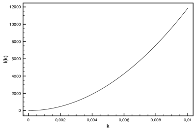
(a) Small range of $k<k_{\rm c}$.

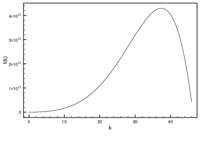
(b) Wide range of $k$ including $k>k_{\rm c}$.

Figure 1: Plots of $I(k)$ for the illustrative choice of $k_{\rm c}=10$.

Then, using the above, and noting that we must use the input to the temporal integrals as

$$a\propto\left(\frac{\eta}{\eta_{0}}\right)\,,\hskip 28.45274pt\rho_{0}=\rho_{0\rm ini}\left(\frac{\eta}{\eta_{0}}\right)^{-4}\,,$$ (45)

we obtain the power spectrum for the vorticity, for general $k_{\rm c}$ as

$${\mathcal{P}}_{\omega}(k,\eta) =\frac{81}{256}k_{0}^{5}\frac{\eta^{2}}{4\pi^{4}}\frac{1}{\rho_{0\rm ini}^{4}}\ln^{2}\left(\frac{\eta}{\eta_{0}}\right)\Bigg{(}\frac{\alpha(k_{0})}{1-\alpha(k_{0})}\Bigg{)}^{2}k_{0}^{-12}\Delta_{\mathcal{R}}^{8}\rho_{0\rm ini}^{4}k_{\rm c}^{5}\Bigg{[}\frac{16}{135}\frac{k_{\rm c}^{4}}{k_{0}^{4}}\left(\frac{k}{k_{0}}\right)^{7}+\frac{12}{245}\frac{k_{\rm c}^{2}}{k_{0}^{2}}\left(\frac{k}{k_{0}}\right)^{9}-\frac{4}{1575}\left(\frac{k}{k_{0}}\right)^{11}\Bigg{]}\,,$$ (46)

and on substituting in values from Ref. WMAP7 , taking a conservative estimate for $\alpha(k_{0})$, being 10 per cent of the upper bound

$${\mathcal{P}}_{\omega}(k,\eta) =\eta^{2}\ln^{2}\left(\frac{\eta}{\eta_{0}}\right)\Bigg{[}0.87\times 10^{-12}k_{\rm c}^{9}\left(\frac{k}{k_{0}}\right)^{7}{\rm Mpc^{11}}+3.73\times 10^{-18}k_{\rm c}^{7}\left(\frac{k}{k_{0}}\right)^{9}{\rm Mpc^{9}}$$

$$\qquad\qquad\qquad\qquad\qquad-7.71\times 10^{-25}k_{\rm c}^{5}\left(\frac{k}{k_{0}}\right)^{11}{\rm Mpc^{7}}\Bigg{]}\,,$$ (47)

and for our above choice of $k_{\rm c}=10{\rm Mpc}^{-1}$,

$${\mathcal{P}}_{\omega}(k,\eta)=\eta^{2}\ln^{2}\left(\frac{\eta}{\eta_{0}}\right)\Bigg{[}0.87\times 10^{-2}\left(\frac{k}{k_{0}}\right)^{7}+3.73\times 10^{-11}\left(\frac{k}{k_{0}}\right)^{9}-7.71\times 10^{-20}\left(\frac{k}{k_{0}}\right)^{11}\Bigg{]}{\rm Mpc^{2}}\,.$$ (48)

IV Discussion and conclusion

In this paper we have obtained the first realistic calculation of the amount of vorticity generated at second order in cosmological perturbation theory by allowing for a non-adiabatic pressure perturbation, as would be the case in a multi-field or multi-fluid system. By solving the governing equations at first order, we have been able to obtain an approximate input power spectrum for the energy density perturbation. Then, making the ansatz that the non-adiabatic pressure perturbation has a bluer spectrum than that of the energy density in order to keep the non-adiabatic pressure sub-dominant on all scales, we obtain an analytical result for the vorticity. Our results show that the vorticity power spectrum has a non-negligible magnitude which depends on the cut off, $k_{\rm c}$ and the chosen parameters. As this is a second order effect the magnitude is somewhat surprising. We have also shown that the result has a dependence on the wavenumber to the power of at least seven for the choice $\alpha=2$. Therefore the amplification due to the large power of $k$ is huge, rendering the vorticity not only possibly observable but also important for the general understanding of the physical processes taking place in the early universe.

As discussed above, we have only approximated the input power spectra. This approximation necessarily only holds for some time and some range of wavenumbers. The next step will be to solve the system of equations numerically, both the vorticity evolution equations and the input power spectra. This can be done for various settings, e.g. by calculating ${\delta P_{\rm{nad}}}$ from multi-field scalar field model Gordon:2000hv at or during the end of inflation, or for multi-fluid system during later epochs, evolving $\delta\rho$ and using Eq. (14).

One prospect for observing early universe vorticity is in the B-mode polarisation of the CMB. Both vector and tensor perturbations produce B-mode polarisation, but at linear order such vector modes decay with the expansion of the universe. However, vector modes produced by gradients in energy density and entropy perturbations, such as those discussed in this work, will source B-mode polarisation at second order. Furthermore, recently it has been noted that vector perturbations in fact generate a stronger B-mode polarisation that tensor modes with the same amplitude GarciaBellido:2010if . Therefore, it is feasible for vorticity to be observed by future surveys. Finally, an important consequence of vorticity is the generation of magnetic fields, and so early universe vorticity could play a crucial role in determining the origin of primordial magnetic fields. We will investigate this in a future publication inprep .

- (1) E. M. Lifshitz, J. Phys. (USSR) 10, 116 (1946).
- (2) W. B. Bonnor Mon. Not. Roy. Astron. Soc. 117, 104 (1957).
- (3) K. Tomita, Prog. Theor. Phys. 37, 831 (1967); Prog. Theor. Phys. 45, 1747 (1971); Prog. Theor. Phys. 47, 416 (1972).
- (4) V. F. Mukhanov, H. A. Feldman and R. H. Brandenberger, Phys. Rept. 215 (1992) 203.
- (5) J. M. Bardeen, Phys. Rev. D 22, 1882 (1980).
- (6) H. Kodama and M. Sasaki, Prog. Theor. Phys. Suppl. 78, 1 (1984).
- (7) R. Durrer, Fund. Cosmic Phys. 15, 209 (1994) [arXiv:astro-ph/9311041].
- (8) M. Tegmark et al. [SDSS Collaboration], Phys. Rev. D 74 (2006) 123507 [arXiv:astro-ph/0608632].
- (9) E. Komatsu et al., arXiv:1001.4538 [astro-ph.CO].
- (10) [Planck Collaboration], arXiv:astro-ph/0604069.
- (11) N. Bartolo, E. Komatsu, S. Matarrese and A. Riotto, Phys. Rept. 402, 103 (2004) [arXiv:astro-ph/0406398].
- (12) K. Nakamura, Prog. Theor. Phys. 113, 481 (2005) [arXiv:gr-qc/0410024].
- (13) K. A. Malik and D. R. Matravers, Class. Quant. Grav. 25, 193001 (2008) [arXiv:0804.3276 [astro-ph]].
- (14) K. A. Malik and D. Wands, Phys. Rept. 475 (2009) 1 [arXiv:0809.4944 [astro-ph]].
- (15) M. Bruni, S. Matarrese, S. Mollerach and S. Sonego, Class. Quant. Grav. 14 (1997) 2585 [arXiv:gr-qc/9609040].
- (16) H. Noh and J. c. Hwang, Phys. Rev. D 69, 104011 (2004).
- (17) A. J. Christopherson and K. A. Malik, JCAP 0911 (2009) 012 [arXiv:0909.0942 [astro-ph.CO]].
- (18) S. Mollerach, D. Harari and S. Matarrese, Phys. Rev. D 69 (2004) 063002 [arXiv:astro-ph/0310711].
- (19) K. N. Ananda, C. Clarkson and D. Wands, Phys. Rev. D 75 (2007) 123518 [arXiv:gr-qc/0612013].
- (20) D. Baumann, P. J. Steinhardt, K. Takahashi and K. Ichiki, Phys. Rev. D 76 (2007) 084019 [arXiv:hep-th/0703290].
- (21) H. Assadullahi and D. Wands, Phys. Rev. D 79 (2009) 083511 [arXiv:0901.0989 [astro-ph.CO]].
- (22) T. C. Lu, K. Ananda, C. Clarkson and R. Maartens, JCAP 0902 (2009) 023 [arXiv:0812.1349 [astro-ph]].
- (23) A. J. Christopherson, K. A. Malik and D. R. Matravers, Phys. Rev. D 79 (2009) 123523 [arXiv:0904.0940 [astro-ph.CO]].
- (24) M. Giovannini, A primer on the physics of the cosmic microwave background, Hackensack, USA: World Scientific (2008).
- (25) A. R. Liddle and D. H. Lyth, Cosmological inflation and large-scale structure, Cambridge, UK: Univ. Pr. (2000).
- (26) A. Lewis, Phys. Rev. D 70 (2004) 043518 [arXiv:astro-ph/0403583].
- (27) L. Hollenstein, C. Caprini, R. Crittenden and R. Maartens, Phys. Rev. D 77 (2008) 063517 [arXiv:0712.1667 [astro-ph]].
- (28) A. J. Christopherson and K. A. Malik, Phys. Lett. B 675 (2009) 159 [arXiv:0809.3518 [astro-ph]].
- (29) I. A. Brown, arXiv:1005.2982 [astro-ph.CO].
- (30) C. Gordon, D. Wands, B. A. Bassett and R. Maartens, Phys. Rev. D 63, 023506 (2001) [arXiv:astro-ph/0009131].
- (31) J. Garcia-Bellido, R. Durrer, E. Fenu, D. G. Figueroa and M. Kunz, arXiv:1003.0299 [astro-ph.CO].
- (32) A. J. Christopherson, K. A. Malik and D. R. Matravers, (in preparation).
- (33) K. Peeters, Comput. Phys. Commun. 176 (2007) 550 [arXiv:cs/0608005], K. Peeters, arXiv:hep-th/0701238.