Second order cross-correlation between kSZ and 21 cm fluctuations from the EoR

Abstract

The measurement of the brightness temperature fluctuations of neutral hydrogen 21 cm lines from the Epoch of Reionisation (EoR) is expected to be a powerful tool for revealing the reionisation process. We study the 21 cm cross-correlation with Cosmic Microwave Background (CMB) temperature anisotropies, focusing on the effect of the patchy reionisation. We calculate, up to second order, the angular power spectrum of the cross-correlation between 21 cm fluctuations and the CMB kinetic Sunyaev-Zel’dovich effect (kSZ) from the EoR, using an analytical reionisation model. We show that the kSZ and the 21 cm fluctuations are anti-correlated on the scale corresponding to the typical size of an ionised bubble at the observed redshift of the 21 cm fluctuations. The amplitude of the angular power spectrum of the cross-correlation depends on the fluctuations of the ionised fraction. Especially, in a highly inhomogeneous reionisation model, the amplitude reaches the order of $100~{}\mu{\rm K}^{2}$ at $\ell\sim 3000$. We also show that second order terms may help in distinguishing between reionisation histories.

1 Introduction

The Epoch of Reionisation (EoR) is an essential milestone in the formation and evolution of cosmic structure. The first luminous objects produced in collapsed dark matter halos in the early universe ($z\sim 20$) started to reionise the inter galactic medium (IGM) which was neutral after recombination. Currently we have only a few observations for the EoR. The first one is the Ly-$\alpha$ absorption measurement towards high redshift QSOs which probes the fraction of neutral hydrogen along the line of sight (Fan et al., 2006), and the second one is the large-scale CMB polarisation (Komatsu et al., 2010). These observations indicate that the IGM was fully ionised by redshift $z\sim 6$. The recent HST observations found large samples of Lyman break galaxies (LBGs) at high redshifts, $7\lesssim z\lesssim 10$ (Bouwens et al., 2010). Bouwens et al. (2010) have studied reionisation with a galaxy model based on these data. Their results suggested that, in addition to such high redshift LBGs, other reionisation sources, for example, faint galaxies and population III stars, are required to match the optical depth of the WMAP seven-year data.

While, current observational data for the EoR are insufficient to study the details of the EoR. In recent years, several observations of signals from the EoR have been suggested to obtain further information about the EoR, for example fluctuations of the neutral hydrogen 21 cm line (Madau et al. 1997, for a review see Furlanetto et al. 2006), small-scale CMB anisotropies due to the kinetic Sunyaev-Zel’dovich (kSZ; Sunyaev & Zel’dovich 1980; Ostriker & Vishniac 1986; Vishniac 1987, for a review see Aghanim et al. 2008), and Ly-$\alpha$ damping of high redshift QSOs and gamma ray bursts (Miralda-Escudé, 1998; Barkana & Loeb, 2004). While the latter can provide us with information about the end of the EoR, the former two are expected to probe the IGM during the EoR. The LOFAR, MWA and SKA are being installed or designed for the measurement of 21 cm line fluctuations, while telescopes such as ACT, SPT and OLIMPO (Masi et al., 2008) will be used to detect and measure the kSZ signal.

Although both auto-correlations of 21 cm lines and CMB anisotropies during the EoR are good probes of the EoR, the cross-correlation between 21 cm fluctuations and the CMB anisotropies created during the EoR is also expected to be useful to study the history of the EoR. The cross-correlation has a potential to provide additional information other than their respective auto-correlations. Besides, the cross-correlation decreases the statistic errors caused by the foreground and the systematic effects, as compared to their auto-correlation. There are several analytical or numerical works about the cross-correlation between CMB and 21 cm fluctuations during the EoR. Alvarez et al. (2006) and Adshead & Furlanetto (2008) computed the expected signal on large scales ($\ell\sim 100$) by analytically calculating the cross-correlation between 21 cm fluctuations and the CMB Doppler anisotropies in the linear regime of the cosmological perturbations. Tashiro et al. (2010) studied the detectability of these signals by LOFAR, MWA and SKA. On small scales ($\ell>1000$), because the dominant contributions of CMB anisotropies come from the kSZ effect due to the patchiness of the ionised medium, Cooray (2004) has partially studied the cross-correlation with kSZ anisotropies and the second order 21 cm fluctuations in a simple reionisation model. He has also investigated the higher order cross-correlation by calculating the bispectrum. Slosar et al. (2007) have also done the study of the 21 cm cross-correlation with the CMB SZ effect which is caused by hot electrons in the first supernovae remnants during the EoR. Since reionisation is a complex physical process, numerical simulations play an important role in the studies of the 21 cm cross-correlation with CMB temperature anisotropies. Numerical works by Jelić et al. (2010) and Salvaterra et al. (2005), focus especially on the small-scale cross-correlation due to the patchy reionisation. Additionally, the 21 cm cross-correlation with CMB polarisation has been calculated by Tashiro et al. (2008) and Dvorkin et al. (2009).

In this paper, we study the cross-correlation between kSZ anisotropies and the second order 21 cm fluctuations during the EoR analytically. Cooray (2004) has studied this cross-correlation in the simple analytical reionisation model where the fluctuations of the ionisation fraction are linearly related to the density fluctuations. He concluded that the cross-correlation cannot appear due to the geometric cancellation occurring between the velocity and the density fluctuations. However, the kSZ effect depends strongly on the evolution of the ionisation bubbles, and numerical studies of the cross-correlation between 21 cm and kSZ anisotropies also shows that patchy reionisation generates signals on small scales (Salvaterra et al., 2005). Therefore, we revisit this issue with the analytical model of McQuinn et al. (2005) which produces a reionisation history similar to that found in recent numerical simulations.

The outline of our paper is the following. In Sec. II, we give the analytical form of the second order cross-correlation between kSZ anisotropies and 21 cm fluctuations. In Sec. III, we give a short description of the analytical reionisation model based on McQuinn et al. (2005). In Sec. IV, we show the angular power spectrum of the second order cross-correlation and we discuss the detectability in the case of the SKA sensitivity. Section V is devoted to the conclusions. Throughout the paper, we use the concordance cosmological parameters for a flat cosmological model, i.e. $h=0.73\ (H_{0}=h\times 100{\rm~{}km/s/Mpc})$, $T_{0}=2.725$K, $\Omega_{\rm b}=0.05$, $\Omega_{\rm m}=0.27$ and $\sigma_{8}=0.9$.

2 The second order cross-correlation

In this section, we calculate the angular power spectrum of the cross-correlation between 21 cm fluctuations and kSZ anisotropies during the EoR at the second order in the fluctuations. For simplicity, we assume that both fluctuation fields are isotropic statistically. Under this assumption, the angular power spectrum of the cross-correlation $C_{\ell}$ is given by

$$\langle a_{\ell_{1}m_{1}}^{*{\rm kSZ}}a_{\ell_{2}m_{2}}^{21}\rangle=\delta_{\ell_{1}\ell_{2}}^{D}\delta_{m_{1}m_{2}}^{D}C_{\ell_{1}},$$ (1)

where $a_{\ell_{1}m_{1}}^{{\rm kSZ}}$ and $a_{\ell_{2}m_{2}}^{21}$ are the multipole components of the CMB temperature anisotropies and 21 cm fluctuations during the EoR.

2.1 kSZ CMB anisotropies

During the EoR, secondary CMB temperature anisotropies are caused by the kinetic SZ effect. Their expression is

$$T_{\rm kSZ}(\hat{\bm{n}})=-T_{\rm cmb}\int^{\eta_{0}}~{}d\eta~{}g(\eta)\hat{\bm{n}}\cdot{\bm{v}}(\eta,\hat{\bm{n}}),$$ (2)

where ${\bm{v}}$ is the baryon velocity field, $g(\eta)$ is the visibility function at the conformal time $\eta$, and the present value of the conformal time is $\eta_{0}$. The visibility function is given by $g(\eta)=\dot{\tau}e^{-\tau}$ where $\tau$ is the optical depth of Thomson scattering from $\eta$ to today and $\dot{\tau}=\sigma_{T}x_{i}n_{\rm H}$ with $\sigma_{T}$ the cross section of Thomson scattering, $x_{i}$ the ionised fraction, and $n_{\rm H}$ the neutral hydrogen density (we ignore the ionisation of helium).

We can decompose $x_{i}$ and $n_{\rm H}$ into the background and fluctuation values,

$$n_{H}=\bar{n}_{H}(1+\delta),\qquad x_{i}=\bar{x}_{i}(1+\delta_{x}),$$ (3)

where the symbols with a bar represent the background values. In Eq. (3), since we assume that the hydrogen density follows the dark matter density on scales much bigger than the baryonic Jeans length, $\delta$ is the total matter density fluctuation field.

Substituting Eq. (3) into Eq. (2), we obtain

$$T_{\rm kSZ}(\hat{\bm{n}})=-T_{\rm cmb}\int~{}d\eta~{}{\bar{g}}(\eta)\hat{\bm{n}}\cdot{\bm{v}}(\eta,\hat{\bm{n}})~{}(1+\delta(\eta,\hat{\bm{n}})+\delta_{x}(\eta,\hat{\bm{n}})+\delta(\eta,\hat{\bm{n}})\delta_{x}(\eta,\hat{\bm{n}})).$$ (4)

We focus on the second order part in Eq. (4), which can be written in terms of the Fourier components of the fluctuations as

$$\delta T_{\rm kSZ}(\hat{\bm{n}})=-iT_{\rm cmb}\int d\eta\int{d^{3}{\bm{k}}\over(2\pi)^{3}}\int{d^{3}{\bm{k}^{\prime}}\over(2\pi)^{3}}{\bar{g}}(\eta)\frac{\hat{\bm{n}}\cdot({\bm{k}}-{\bm{k}}^{\prime})}{|{\bm{k}}-{\bm{k}}^{\prime}|^{2}}\dot{\delta}(\eta,{\bm{k}}-{\bm{k}}^{\prime})(\delta(\eta,{\bm{k}}^{\prime})+\delta_{x}(\eta,{\bm{k}}^{\prime}))\exp[i(\eta_{0}-\eta)(\hat{\bm{n}}\cdot{\bm{k}})],$$ (5)

where we use the relation ${\bm{r}}=(\eta_{0}-\eta)\hat{\bm{n}}$, and we relate the velocity to $\delta$ by the continuity equation in the cosmological linear perturbation theory

$${\bm{v}}=i\frac{\bm{k}}{k^{2}}\dot{\delta}(\eta,k),$$ (6)

where the dot represents the derivative with respect to $\eta$.

Our final aim is to obtain the angular power spectrum of the cross-correlation. Therefore, we consider the spherical harmonic decomposition of Eq. (5), $a_{\ell m}^{\rm kSZ}=\int d\hat{\bm{n}}\delta T_{\rm kSZ}(\hat{\bm{n}})Y_{\ell}^{m}$. The spherical harmonic coefficients of the kSZ are given by

$$a_{\ell m}^{\rm kSZ} = \sum_{\begin{subarray}{c}\ell^{\prime}m^{\prime}\ell^{\prime\prime}m^{\prime\prime}\\ \ell^{\prime\prime\prime}m^{\prime\prime\prime}m^{\prime\prime\prime\prime}\end{subarray}}\int d\eta\int{d^{3}{\bm{k}}_{1}\over(2\pi)^{3}}\int{d^{3}{\bm{k}}_{2}\over(2\pi)^{3}}$$ (7)

$$\quad\times A_{\ell\ell^{\prime}\ell^{\prime\prime}\ell^{\prime\prime\prime}1}^{mm^{\prime}m^{\prime\prime}m^{\prime\prime\prime}m^{\prime\prime\prime\prime}}(\eta)\dot{\delta}(\eta,{\bm{k}}_{1})(\delta(\eta,{\bm{k}}_{2})+\delta_{x}(\eta,{\bm{k}}_{2})){j_{\ell^{\prime}}(k_{1}r)\over k_{1}}j_{\ell^{\prime\prime}}(k_{2}r)Y^{m^{\prime\prime\prime}}_{\ell^{\prime\prime\prime}}(\hat{\bm{k}}_{1})Y_{\ell^{\prime\prime}}^{m^{\prime\prime}}(\hat{\bm{k}}_{2}),$$

where we replaced ${\bm{k}}$ and ${\bm{k}}^{\prime}$ by ${\bm{k}}_{1}\equiv{\bm{k}}-{\bm{k}}^{\prime}$ and ${\bm{k}}_{2}\equiv{\bm{k}}^{\prime}$, and

$$A_{\ell\ell^{\prime}\ell^{\prime\prime}\ell^{\prime\prime\prime}1}^{mm^{\prime}m^{\prime\prime}m^{\prime\prime\prime}m^{\prime\prime\prime\prime}}=-i(-1)^{m+m^{\prime}-m^{\prime\prime}+m^{\prime\prime\prime\prime}}{64\pi^{3}\over 3}i^{\ell^{\prime}+\ell^{\prime\prime}}\sqrt{3(2\ell^{\prime}+1)\over 4\pi(2\ell^{\prime\prime\prime\prime}+1)}C^{\ell^{\prime}\ell^{\prime\prime\prime}1}_{-m^{\prime}-m^{\prime\prime\prime}m^{\prime\prime\prime\prime}}C^{\ell^{\prime}\ell^{\prime\prime\prime}1}_{000}M^{-mm^{\prime}-m^{\prime\prime}m^{\prime\prime\prime\prime}}_{\ell\ell^{\prime}\ell^{\prime\prime}1}T_{\rm cmb}\bar{g}(\eta).$$ (8)

Here, $C^{\ell_{1}\ell_{2}\ell}_{m_{1}m_{2}m}$ are the Clebsch-Gordan coefficients and $M^{m_{1}m_{2}m_{3}m_{4}}_{\ell_{1}\ell_{2}\ell_{3}\ell_{4}}$ are the integrals of quadruple spherical harmonics,

$$M^{m_{1}m_{2}m_{3}m_{4}}_{\ell_{1}\ell_{2}\ell_{3}\ell_{4}} = \int d\hat{n}~{}Y^{m_{1}}_{\ell_{1}}(\hat{n})Y^{m_{2}}_{\ell_{2}}(\hat{n})Y^{m_{3}}_{\ell_{3}}(\hat{n})Y^{m_{4}}_{\ell_{4}}(\hat{n})$$ (9)

$$= (-1)^{m_{1}}\sum_{\ell^{\prime}m^{\prime}}\sqrt{(2\ell_{2}+1)(2\ell_{3}+1)(2\ell_{4}+1)\over 16\pi^{2}(2\ell_{1}+1)}C^{\ell_{3}\ell_{4}\ell^{\prime}}_{m_{3}m_{4}m^{\prime}}C^{\ell_{3}\ell_{4}\ell^{\prime}}_{000}C^{\ell_{2}\ell^{\prime}\ell_{1}}_{m_{2}m^{\prime}-m_{1}}C^{\ell_{2}\ell^{\prime}\ell_{1}}_{000}.$$

2.2 21 cm fluctuations

The brightness temperature of the 21 cm line from a redshift $z$ is given as in Madau et al. (1997) by

$$T_{21}(z)=\frac{\tau_{21}}{(1+z)}(T_{\rm s}-T_{\rm CMB})(z),$$ (10)

where $T_{\rm CMB}$ is the CMB temperature and $T_{\rm s}$ is the spin temperature given by the ratio of the number density of hydrogen in the excited state to that of hydrogen in the ground state. The optical depth for the 21 cm line absorption $\tau_{21}$ is

$$\tau_{21}(z)={3c^{3}\hbar A_{10}x_{\rm H}n_{\rm H}\over 16k\nu_{21}^{2}T_{\rm s}H(z)},$$ (11)

where $A_{10}$ is the Einstein A-coefficient, $\nu_{21}$ is the frequency corresponding to the 21 cm wavelength and $x_{\rm H}$ is the fraction of neutral hydrogen, which is written as a function of the ionised fraction $x_{i}=1-x_{\rm H}$. Note that we drop the redshift space distortion by the peculiar velocity fluctuations of neutral hydrogen in Eq. (11), although this effect enhances the 21 cm fluctuations (Bharadwaj & Ali, 2004).

Combining Eq. (3) with Eqs. (10) and (11), we can obtain the observed 21 cm fluctuations at the observed frequency $\nu$. The second order fluctuations which we here focus on is given by

$$\delta T_{21}(\hat{\bm{n}},\nu)=\int~{}d\eta\int{d^{3}{\bm{k}}\over(2\pi)^{3}}{d^{3}{\bm{k}^{\prime}}\over(2\pi)^{3}}W_{21}(\eta,\eta(z_{\rm obs}))T_{0}(z(\eta))\delta(\eta,{\bm{k}}-{\bm{k}}^{\prime})\delta_{H}(\eta,{\bm{k}}^{\prime})\exp[i(\eta_{0}-\eta)(\hat{\bm{n}}\cdot{\bm{k}})],$$ (12)

where $W_{21}(\eta,\eta(z))$ is the spectral response function of the observation experiment, normalised as $\int d\eta W_{21}(\eta,\eta(z))=1$ and centred at $\eta(z)$, the redshift $z_{\rm obs}$ is related to the frequency $\nu$ as $\nu=\nu_{21}/(1+z_{\rm obs})$, $\delta_{H}\equiv(x_{H}-\bar{x}_{H})/\bar{x}_{H}$ and $T_{0}$ is a normalisation temperature factor given by

$$T_{0}(z)=23\left({\Omega_{\rm b}h^{2}\over 0.02}\right)\left[\left({0.15\over\Omega_{\rm m}h^{2}}\right)\left({1+z\over 10}\right)\right]^{1/2}\left({T_{\rm s}-T_{\rm cmb}\over T_{\rm s}}\right)~{}{\rm mK}.$$ (13)

The spin temperature is determined by three couplings with CMB, IGM gas and Ly-$\alpha$ photons. In the EoR, Ly-$\alpha$ photons emitted from ionising sources couple the spin temperature with the IGM gas temperature (Ciardi & Madau, 2003). Meanwhile, since the IGM gas is heated up quickly by Ly-$\alpha$ and X-ray photons from stars and QSOs, the IGM gas temperature is much higher than the CMB temperature during reionisation. Therefore, we can assume $T_{\rm s}\gg T_{\rm cmb}$ during the EoR in Eq. (13).

Taking the harmonic decomposition, we obtain the spherical harmonic coefficients of the 21 cm fluctuations,

$$a_{\ell m}^{21}=\sum_{\ell^{\prime}m^{\prime}}\sum_{\ell^{\prime\prime}m^{\prime\prime}}\int~{}d\eta\int{d^{3}{\bm{k}_{1}}\over(2\pi)^{3}}\int{d^{3}{\bm{k}_{2}}\over(2\pi)^{3}}B^{mm^{\prime}m^{\prime\prime}}(\eta)\delta(\eta,{\bm{k}}_{1})\delta_{H}(\eta,{\bm{k}}_{2})j_{\ell^{\prime}}(k_{1}r)j_{\ell^{\prime\prime}}(k_{2}r)Y_{\ell^{\prime}}^{m^{\prime}*}(\hat{\bm{k}}_{1})Y_{\ell^{\prime\prime}}^{m^{\prime\prime}*}(\hat{\bm{k}}_{2}),$$ (14)

where

$$B^{mm^{\prime}m^{\prime\prime}}(\eta)=16\pi^{2}i^{\ell^{\prime}+\ell^{\prime\prime}}W_{21}(\eta)T_{0}(\eta)M^{m^{\prime}m^{\prime\prime}-m}_{\ell^{\prime}\ell^{\prime\prime}\ell}.$$ (15)

Here $M^{m_{1}m_{2}m_{3}}_{\ell_{1}\ell_{2}\ell_{3}}$ is the integral of triple spherical harmonics,

$$M^{m_{1}m_{2}m_{3}}_{\ell_{1}\ell_{2}\ell_{3}} = \int d\hat{n}~{}Y^{m_{1}}_{\ell_{1}}(\hat{n})Y^{m_{2}}_{\ell_{2}}(\hat{n})Y^{m_{3}}_{\ell_{3}}(\hat{n})$$ (16)

$$= (-1)^{m_{1}}\sqrt{(2\ell_{2}+1)(2\ell_{3}+1)\over 4\pi(2\ell_{1}+1)}C^{\ell_{2}\ell_{3}\ell_{1}}_{m_{2}m_{3}-m_{1}}C^{\ell_{2}\ell_{3}\ell_{1}}_{000},$$

where $m_{1}+m_{2}=m_{3}$.

2.3 The cross-correlation

The second order cross-correlation is given by substituting Eqs. (7) and (14) into Eq. (1). We obtain

$$C^{{\rm kSZ}-21}_{\ell} = -\sum_{\ell^{\prime}_{1}m^{\prime}_{1}}\sum_{\ell^{\prime\prime}_{1}m^{\prime\prime}_{1}}\sum_{\begin{subarray}{c}\ell^{\prime}_{2}m^{\prime}_{2}\\ \ell^{\prime\prime}_{2}m^{\prime\prime}_{2}m^{\prime\prime\prime}_{2}\\ \ell^{\prime\prime\prime\prime}_{2}m^{\prime\prime\prime\prime}_{2}\end{subarray}}\int d\eta\int d\eta^{\prime}\int{d^{3}{\bm{k}_{1}}\over(2\pi)^{3}}\int{d^{3}{\bm{k}_{2}}\over(2\pi)^{3}}\int{d^{3}{\bm{k}_{1}^{\prime}}\over(2\pi)^{3}}\int{d^{3}{\bm{k}_{2}^{\prime}}\over(2\pi)^{3}}$$ (17)

$$\langle\delta^{*}(\eta,{\bm{k}}_{1})\delta_{x}^{*}(\eta,{\bm{k}}_{2})\dot{\delta}(\eta^{\prime},{\bm{k}}^{\prime}_{1})(\delta(\eta^{\prime},{\bm{k}}^{\prime}_{2})+\delta_{x}(\eta^{\prime},{\bm{k}}^{\prime}_{2}))\rangle A_{\ell\ell^{\prime}_{2}\ell^{\prime\prime}_{2}1\ell^{\prime\prime\prime\prime}_{2}}^{mm^{\prime}_{2}m^{\prime\prime}_{2}m^{\prime\prime\prime}_{2}m^{\prime\prime\prime\prime}_{2}}(\eta^{\prime})[B^{m-m^{\prime}_{1}-m^{\prime\prime}_{1}}(\eta)]^{*}$$

$$\times j_{\ell^{\prime}_{1}}(k_{1}r)j_{\ell^{\prime\prime}_{1}}(k_{2}r){j_{\ell^{\prime}_{2}}(k^{\prime}_{1}r^{\prime})\over k^{\prime}_{1}}j_{\ell^{\prime\prime}_{2}}(k^{\prime}_{2}r^{\prime})Y_{\ell^{\prime}_{1}}^{m^{\prime}_{1}*}(\hat{\bm{k}}_{1})Y_{\ell^{\prime\prime}_{1}}^{m^{\prime\prime}_{1}*}(\hat{\bm{k}}_{2})Y^{m^{\prime\prime\prime\prime}_{2}}_{\ell^{\prime\prime\prime\prime}_{2}}(\hat{\bm{k}}^{\prime}_{1})Y_{\ell^{\prime\prime}_{2}}^{m^{\prime\prime}_{2}}(\hat{\bm{k}}^{\prime}_{2}),$$

where $r^{\prime}=\eta_{0}-\eta^{\prime}$ and we use $\delta_{x}=-\delta_{H}$.

Under the assumption that all fluctuation fields are Gaussian, the Wick theorem breaks the ensemble average in Eq. (17) into components with $\langle\delta\delta\rangle$, $\langle\delta_{x}\delta_{x}\rangle$ and $\langle\delta\delta_{x}\rangle$. For the simplification of Eq. (17), we assume that $W_{21}(z)=\delta(z-z_{\rm obs})$. This is a good approximation because, compared to the observed frequency, the spectral resolution is narrow (for example, the spectral resolution in the LOFAR case is less than 1 MHz while the observed frequency is about 150 MHz for $z_{\rm obs}\sim 10$). We can simplify further by using the approximation for the integration of spherical Bessel functions with $\ell\gg 1$,

$$\int dr^{\prime}\int dk~{}k^{2}F(k)j_{\ell}(kr)j_{\ell}(kr^{\prime})\approx\left.\int dr^{\prime}{\pi\over 2}{\delta(r-r^{\prime})\over r^{2}}F(k)\right|_{k=\ell/r}={\pi\over 2}{F(\ell/r)\over r^{2}}.$$ (18)

Finally, we can rewrite the cross-correlation as

$$C^{{\rm kSZ}-21}_{\ell} = -\sum_{\ell_{1}\ell_{2}}{(2\ell_{2}+1)(2\ell_{1}+1)\over 2\pi^{2}(2\ell+1)}|C^{\ell_{1}\ell_{2}\ell}_{000}|^{2}{T_{0}(\eta_{\rm obs})T_{\rm cmb}\over H_{\rm obs}r_{\rm obs}^{2}}{\dot{G}(\eta_{\rm obs})\over G(\eta_{\rm obs})}\bar{g}(\eta_{\rm obs})\int{d{k}}{j_{\ell_{1}}(kr_{\rm obs})}\left.{dj_{\ell_{1}}(kr)\over dr}\right|_{r=r_{\rm obs}}$$ (19)

$$\times\left.\left[\left(P_{\delta x}\left(\eta_{\rm obs},{\ell_{2}\over r}\right)+P_{xx}\left(\eta_{\rm obs},{\ell_{2}\over r}\right)\right)P_{\delta\delta}(\eta_{\rm obs},k)+\left(P_{\delta\delta}\left(\eta_{\rm obs},{\ell_{2}\over r}\right)+P_{\delta x}\left(\eta,{\ell_{2}\over r}\right)\right)P_{\delta x}(\eta_{\rm obs},k)\right]\right|_{r=r_{\rm obs}},$$

where the power spectra $P_{\delta\delta},P_{xx}$ and $P_{\delta x}$ are defined as $\langle\delta(\eta,k_{1})\delta(\eta,k_{2})\rangle=(2\pi)^{3}\delta(k_{1}-k_{2})P_{\delta\delta}(\eta,k_{1})$, $\langle\delta_{x}(\eta,k_{1})\delta_{x}(\eta,k_{2})\rangle=(2\pi)^{3}\delta(k_{1}-k_{2})P_{xx}(\eta,k_{1})$, and $\langle\delta(\eta,k_{1})\delta_{x}(\eta,k_{2})\rangle=(2\pi)^{3}\delta(k_{1}-k_{2})P_{\delta x}(\eta,k_{1})$. In Eq. (19), $G$ is the growth factor of the dark matter density fluctuations which is $\delta(k,\eta)=G(\eta)\delta(k)$ with the present density fluctuations $\delta(k)$. Now, the epoch we are interested in is matter dominated, so that we can assume $G\propto 1/(1+z)$ in terms of the redshift $z$.

In order to calculate the cross-correlation, the power spectra $P_{xx}$ and $P_{\delta x}$ which are determined by the reionisation model are essential. We discuss the analytical reionisation model in the following section.

3 reionisation model

For an analytical reionisation model, we adopt the approach of Furlanetto et al. (2004b) and McQuinn et al. (2005). Ionisation bubbles start to evolve from high density galaxy regions into the voids, as shown in recent numerical simulations (e.g. Trac & Gnedin, 2009, and references therein). Therefore, the mass of ionised gas $m_{\rm ion}$ is associated with the mass of a collapsed object $m_{\rm gal}$ by the Ansatz, $m_{\rm ion}=\zeta m_{\rm gal}$ where $\zeta$ is an ionizing efficiency. The condition for the full ionisation of a region of mass $m$ is that the region contains sufficient sources to self-ionise, i.e. $f_{\rm coll}\geq\zeta^{-1}$, where $f_{\rm coll}$ is the fraction of collapsed halos above the critical mass for collapse, $m_{\rm min}$ (Lacey & Cole, 1993).

This criterion gives the barrier (the density threshold) $\delta_{x}$ for “self-ionisation” which depends on $m$. Furlanetto et al. (2004a) found a reasonable approximation of the barrier in the linear form of the variance of the density fluctuations, $\sigma^{2}(m,z)$, as $B(m,z)=B_{0}+B_{1}\sigma^{2}(m,z)$ where $\sigma(m,z)$ is obtained by smoothing the density field at the scale $m$. Here, $B_{0}=\delta_{c}-\sqrt{2}K(\zeta)\sigma_{\rm min}(z)$ and $B_{1}=\partial\delta_{x}/\partial\sigma^{2}|_{\sigma^{2}=0}$ where $\sigma_{\rm min}(z)$ is the mass dispersion at the minimum mass and redshift $z$ for the collapsed ionisation source.

For the linear barrier $B(m,z)$, the bubble mass function is written as (Sheth, 1998)

$$\frac{dn(m)}{dm}dm=\sqrt{\frac{2}{\pi}}\frac{\bar{\rho}}{m^{2}}\left|\frac{d\log\sigma}{d\log m}\right|\frac{B_{0}}{\sigma(m)}\exp\left[-\frac{B^{2}(m,z)}{2\sigma^{2}(m)}\right]dm\,,$$ (20)

where $\bar{\rho}$ is the mean mass density of the Universe.

The smallest bubble mass is given by $\zeta m_{\rm min}$. Therefore, we can obtain the mean ionised fraction (volume averaged) $\bar{x}_{i}$ as

$$\bar{x}_{i}=\int_{\zeta m_{\rm min}}V(m)\frac{dn(m)}{dm}dm=\frac{1}{2}e^{-2B_{0}B_{1}}{\rm erfc}\left(\frac{B_{0}-B_{1}\sigma_{\zeta}^{2}}{\sqrt{2\sigma_{\zeta}^{2}}}\right)+\frac{1}{2}{\rm erfc}\left(\frac{B_{0}+B_{1}\sigma_{\zeta}^{2}}{\sqrt{2\sigma_{\zeta}^{2}}}\right),$$ (21)

where $\sigma_{\zeta}=\sigma(\zeta m,z)$ and $V(m)$ is the comoving volume of a bubble with mass $m$.

In the case of a linear barrier, the linear bias of a source of mass $m$ is given by (McQuinn et al., 2005)

$$b(m)=1+{B(m)/\sigma^{2}(m)-1/B_{0}\over D(z)}.$$ (22)

Therefore, the mean bias of the bubble $\bar{b}(m)$ is obtained from

$$\bar{b}=\bar{x}_{i}^{-1}\int dm\,b(m)V(m)\frac{dn(m)}{dm}.$$ (23)

In this reionisation model, the free parameters for the model are $\zeta$ and $m_{\rm min}$. Here we take two parameter sets which are motivated from numerical simulations: “stars” model and “QSOs” model (Jelić et al., 2010). In both models, the ionised fraction reaches $\bar{x}_{i}=0.5$ at $z=11$, in order to agree with the WMAP results.

In the “stars” model, we assume that stars are responsible for reionisation. We take a low efficiency $\zeta\approx 40$ which is reasonable for normal star formation and assume that the minimum mass corresponds to a virial temperature of $10^{4}$ K, above which cooling by atomic hydrogen becomes efficient.

In the “QSOs” model, we assume that the reionisation history is faster and the bubble size is larger compared to those in the “stars” model. Therefore, we set high a virial temperature ($5\times 10^{4}$ K) and a high efficiency $\zeta\approx 200$. The candidates for the ionisation sources are massive stars and QSOs.

We show the evolution of the ionised fraction for each model in Fig. 1. From Eq. (20), we can obtain the bubble size distribution $Vdn/dR$ as a function of the comoving size $R$ of a bubble under the assumption that the bubbles are spherical. We plot the results in Fig. 2.

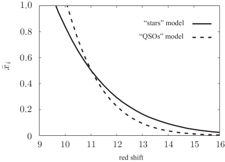
Figure 1: Evolution of the mean ionised fraction. The solid and dotted lines represent $\bar{x}_{i}$ in the “stars” and “QSOs” models, respectively.

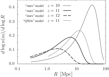
Figure 2: Ionised bubble comoving size distribution. The dotted, solid and dashed lines represent the distributions in the “stars” model at $z=10$, $z=11$ and $z=12$, respectively. The ionised fractions are $\bar{x}_{i}=0.8$ at $z=10$, $\bar{x}_{i}=0.5$ at $z=11$ and $\bar{x}_{i}=0.3$ at $z=12$. We also plot the distribution in the “QSOs” model at $z=11$ as the thin solid line. The left side of each line ends at $R(\zeta m_{\rm min})$ where $\zeta m_{\rm min}$ is the minimum mass of the ionised region.

3.1 The two-point correlation function $\xi_{xx}(r)$

In order to obtain the power spectra $P_{xx}$ and $P_{\delta x}$ in Eq. (19), we need to compute the correlation function $\xi_{xx}(r)=\langle x_{i}({\bm{x}}_{1})x_{i}({\bm{x}}_{2})\rangle-\bar{x}_{i}^{2}$ and $\xi_{\delta x}(r)=\langle\delta({\bm{x}}_{1})x_{i}({\bm{x}}_{2})\rangle$ where the points ${\bm{x}}_{1}$ and ${\bm{x}}_{2}$ are separated by $r=|{\bm{x}}_{1}-{\bm{x}}_{2}|$. Here we utilize the analytical correlation functions of McQuinn et al. (2005).

As in the case of the density correlation function in the halo formalism, the correlation function of the ionised fraction $\xi_{xx}(r)$ receives two contributions. One is a one bubble term $P_{1}$ which is the two-point correlation for the case where two points which are separated by $r$ are ionised by the one and same ionisation source, the other is a two bubble term $P_{2}$ which corresponds to the case where two points are ionised by two separate sources. As shown in Fig. 2, the typical size of an ionisation bubble becomes larger than 5 Mpc when the ionised fraction reaches one half. In such regime, where the ionisation bubbles become large, $P_{1}$ is largely dominant and $P_{2}$ can be ignored. Thus, McQuinn et al. (2005) divide the reionisation process into two phases: the early phase and the late phase. In the early phase, both $P_{1}$ and $P_{2}$ are important, while in the late phase, $P_{1}$ is dominant and $P_{2}$ can be ignored. The criterion for these phases is set as $\bar{x}_{i}>0.5$ in order to be in agreement with results from the hybrid approach of analytic modeling and numerical simulations of Zahn et al. (2005). They define the correlation function $\xi_{xx}(r)$ by

$$\xi_{xx}(r) =\left\{\begin{array}[]{l l}(1-\bar{x}_{i})\,P_{1}(r)&{\rm when~{}}\bar{x}_{i}>0.5,\\ P_{1}(r)+P_{2}(r)-\bar{x}_{i}^{2}&{\rm otherwise},\end{array}\right.$$ (26)

where

$$P_{1}(r) = \int dm\,{dn(m)\over dm}V_{0}(m,r),$$ (27)

$$P_{2}(r) = \int dm_{1}{dn(m_{1})\over dm}\int d^{3}{\bm{r}}_{1}\int dm_{2}{dn(m_{2})\over dm}\int d^{3}{\bm{r}}_{2}[1+\xi({\bm{r}}_{1}-{\bm{r}}_{2}|m_{1},m_{2})].$$ (28)

Here, $\xi(r|m_{1},m_{2})$ is the excess probability to have a bubble of mass $m_{1}$ at the distance $r$ from a bubble of mass $m_{2}$. For the simplicity of the calculation, it is assumed that $\xi(r|m_{1},m_{2})$ can be written in terms of the correlation function of the matter density $\xi_{\delta\delta}$ as $\xi(r|m_{1},m_{2})=\bar{b}\xi_{\delta\delta}({\rm max}(r,R_{1}+R_{2}))$ where $R_{1}(m_{1})$ and $R_{2}(m_{2})$ are the bubble radii.

In order to calculate the volume in Eqs. (27) and (28) analytically, all ionisation bubbles are assumed spherical. Therefore, $V_{0}(m,r)$ is the volume within a sphere of mass $m$ that can encompass two points separated by a distance $r$. For the volume integration in Eq. (28), McQuinn et al. (2005) adopt the overlapping conditions: (1) $m_{1}$ cannot ionize $r_{2}$, and $m_{2}$ cannot ionize $r_{1}$; (2) the center of $m_{2}$ cannot lie inside $m_{1}$, but any other part of $m_{2}$ can touch $m_{1}$, and vice versa.

3.2 The two-point cross-correlation function $\xi_{\delta x}(r)$

As in the case of $\xi_{xx}(r)$, the two-point cross-correlation $\xi_{\delta x}(r)$ has two contributions, $P_{\rm in}$ and $P_{\rm out}$. The contribution $P_{\rm in}$ corresponds to the case of both points being contained within the same ionised bubble. Following McQuinn et al. (2005), it is written as

$$P_{\rm in}(r) = \int dm{dn(m)\over dm}V_{0}(m,r)\int dm_{h}\frac{m_{h}}{\rho}{dn_{h}(m_{h}|m)\over dm_{h}}$$ (29)

$$= \int dm{dn(m)\over dm}V_{0}(m,r)[1+B(m,z)],$$

where the last line in Eq. (29) is obtained by using the fact that the inner integral is the mean over-density of the bubble $1+\delta_{B}$ and $\delta_{B}$ is $B(m,z)$ at linear order.

The contribution $P_{\rm out}$ corresponds to the case when one point is outside the ionised bubble of the other point. McQuinn et al. (2005) give $P_{\rm out}$ in terms of the mean bias for halos $\bar{b}_{h}$,

$$P_{\rm out}(r) = \bar{x}_{i}-\int dm{dn(m)\over dm}V_{0}(m,r)+\int dm{dn(m)\over dm}\int d^{3}{\bm{r}}_{\rm b}[\bar{b}_{h}\bar{b}\xi_{\delta\delta}({\bm{r}}-{\bm{r}}_{\rm b})].$$ (30)

where $dn_{h}(m_{h}|m)/dm_{h}$ is the conditional mass function. In Eq. (30), the integration range of ${\bm{r}}_{\rm b}$ is over all bubbles which ionise the point ${\bm{r}}_{\rm b}$ but not the other point separated by ${\bm{r}}$ from ${\bm{r}}_{\rm b}$. For simplicity, $\xi_{\delta\,\delta}$ is evaluated at the separation ${\rm max}[R(m),r]$.

As the reionisation proceeds and the typical size of an ionised bubble becomes large, the term $P_{out}$ becomes unimportant as compared to $P_{in}$. Therefore, the computation of $\xi_{\delta x}$ is divided into two phases again,

$$\xi_{\delta x}(r) =\left\{\begin{array}[]{l l}P_{\rm in}-P_{1}&{\rm when~{}}\bar{x}_{i}>0.5,\\ P_{\rm in}+P_{\rm out}-\bar{x}_{i}&{\rm otherwise},\end{array}\right.$$ (33)

where we assume that $P_{\rm in}$ is dominant in large $\bar{x}_{i}$ ($\bar{x}_{i}>0.5$) and we subtract $P_{1}$ given by Eq. (29) from $P_{\rm in}$ which is the correlation between $x_{i}$ and $\rho/\bar{\rho}$.

4 Results and discussion

We calculate the angular power spectrum of the cross-correlation described in Eq. (19) in the two models, “stars” and “QSOs”. First, we show the results in the “stars” model in Fig. 3. In this model, the mean ionised fraction is $0.3$, $0.5$ and $0.8$ at $z=12$, $z=11$ and $z=10$, respectively. The signal of the cross-correlation between kSZ and 21 cm fluctuations exhibits an anti-correlation on small scales ($\ell>1000$). As mentioned in Cooray (2004), there is a geometric cancellation in the cross-correlation. This cancellation is responsible for a suppression of the amplitude of the cross-correlation. However, the cross-correlation has a distinctive oscillatory shape. Especially, we found that the peak position of the anti-correlation represents the typical size of an ionised bubble at each redshift. For example, at $z=11$, the typical size of an ionised bubble is almost $6$ Mpc, as shown in Fig. 2, and the anti-correlation at $z_{\rm obs}=11$ is maximal at the corresponding multipole $\ell\sim 4000$. As the Universe evolves, the typical scale of an ionised bubble becomes larger. The peak position of the anti-correlation shifts accordingly toward smaller values.

The evolution of the cross-correlation amplitude depends on the evolution of $\delta_{x}$ through the power spectra of $P_{xx}$ and $P_{x\delta}$ which evolve rapidly during the EoR. Since the amplitudes of $P_{xx}$ and $P_{x\delta}$ increase as the redshift decreases, the amplitude of the cross-correlation also becomes larger at low redshifts. However, after the average ionisation rate reaches $\bar{x}_{i}\sim 0.9$, the signal of the 21 cm fluctuations becomes weak and the cross-correlation amplitude also starts to decrease.

In Fig. 3, we also plot the first order cross-correlation between 21 cm and CMB Doppler anisotropies calculated by using the same expression as Eq. (15) of Alvarez et al. (2006). The sign of the first order cross-correlation depends on the evolution of $\delta_{x}$. As long as $\delta_{x}$ is small, the ionisation process is homogeneous, and the cross-correlation is negative. On the other hand, in the case of a highly inhomogeneous reionisation, the sign of the cross-correlation is positive. In our reionisation model, the first order cross-correlation at the early phase of reionisation is negative at $\ell<1000$ (see the top and middle panels in Fig. 3). We found the amplitude of the first order cross-correlation at $z_{\rm obs}=11$ is $300~{}\mu{\rm K}^{2}$ at the peak position, $\ell\sim 100$, and decreases rapidly towards zero at large multipoles. As we can see in Fig. 3, the second order kSZ-21 cm cross-correlation dominates the first order cross-correlation at multipoles larger than $\ell=1000$. However, as the ionisation process proceeds, the ionisation fraction is highly inhomogeneous and $\delta_{x}$ is evolved well. As a result, the first order cross-correlation has a positive sign and a high amplitude as shown in the bottom panel of Fig. 3. The first order cross-correlation becomes comparable to the second order kSZ-21 cm cross-correlation even at $\ell\sim 1000$, while the kSZ cross-correlation still dominate the first order cross-correlation and has negative correlation at multipoles higher than $\ell=1000$.

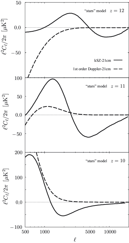
Figure 3: Angular power spectra of the second order cross-correlation in the “stars” model. From top to bottom panels, we plot the angular power spectra at $z_{\rm obs}=12$, $z_{\rm obs}=11$ and $z_{\rm obs}=10$, respectively. The mean ionised fraction is $\bar{x}=0.3$ at $z=12$, $\bar{x}=0.5$ at $z=11$ and $\bar{x}=0.8$ at $z=10$. For reference, we show the first order cross-correlation between the CMB temperature and 21 cm fluctuations as the dotted line in each panel.

Next we show the dependence of the angular cross-correlation power spectrum on the ionisation model in Fig. 4. In the “QSOs” model, the ionisation history is rapid and the typical size of ionised bubbles is large. The amplitude of $P_{xx}$ and $P_{x\delta}$ in the “QSOs” model is larger than in the “stars” model. As a result, in the “QSOs” model, the signal of the cross-correlation is large and the peak position of the anti-correlation appears on small multipoles, as expected. We can therefore conclude that the cross-correlation between kSZ and 21 cm fluctuations at the second order is sensitive to the average size of an ionised bubble. The first order cross-correlation also has a higher amplitude than in the “stars” model because the amplitude depends on the evolution rate of the background ionisation fraction. However, the inhomogeneous contribution coming from the term with $P_{x\delta}$ in Eq. (15) in Alvarez et al. (2006) is partially canceled by the homogeneous one from the term with $P_{\delta\delta}$. As a result, in the highly inhomogeneous “QSOs” reionisation model, the cross-correlation between kSZ and second order 21 cm fluctuations reaches a significant amplitude, compared with the first order cross-correlation at small scales ($\ell\lesssim 1000$).

Figure 4: Dependence of the cross-correlation on the ionisation model. The solid and the dashed lines are the power spectrum for the “stars” model and the “QSOs” model, respectively (see text). We set $z_{\rm obs}=11$ where $\bar{x}=0.5$ in both models. For reference, we plot the first order cross-correlation in each model as the thin lines.

4.1 Detectability

In the previous section, we showed that the peak position of the anti-correlation is related to the typical bubble size at the observed redshift of 21 cm fluctuations. Here, our concern is the detectability of such negative peak in the kSZ-21 cm cross-correlation. In order to investigate the detectability, we calculate the signal-to-noise ratio ($S/N$). For simplicity, we assume that CMB, 21 cm fluctuations and instrumental noise are Gaussian. The total $S/N$ can be calculated as

$$\left({S\over N}\right)^{2}=f_{\rm sky}\sum_{\ell=\ell_{\rm min}}^{\ell_{\rm max}}(2\ell+1){|C_{\ell}^{21-{\rm CMB}}|^{2}\over|C_{\ell}^{21-{\rm CMB}}|^{2}+C_{\ell}^{21}C_{\ell}^{\rm CMB}},$$ (34)

where $f_{\rm sky}$ is the sky fraction common to the two cross-correlated signals, and $C_{\ell}^{\rm CMB}$, $C_{\ell}^{21}$ and $C_{\ell}^{21-{\rm CMB}}$ are the angular power spectra of CMB, 21 cm fluctuation and the cross-correlation between 21 cm and CMB, respectively. In order to focus on the detectability of the signal from the typical bubble size, we set $\ell_{\rm min}=500$ and $\ell_{\rm max}=5000$.

At the multipoles that we are interested in ($\ell>1000$), the dominant CMB signal is due to the thermal SZ effect (Zel’dovich & Sunyaev, 1969). However we can remove this contribution because of the frequency dependence of the SZ effect. Therefore with the assumption that the foreground can be completely removed from the CMB map, the main contribution to $C_{l}^{\rm CMB}$ comes from the primordial CMB anisotropies $C_{\ell}^{\rm pri}$ and the noise of the instrument $N_{\ell}^{\rm CMB}$. We can write $C_{\ell}^{\rm CMB}$ as

$$C_{\ell}^{\rm CMB}=C_{\ell}^{\rm pri}\exp(-\ell^{2}\sigma_{\rm CMB}^{2}/2)+N_{\ell}^{\rm CMB},$$ (35)

where we assume the beam profile of CMB observation is Gaussian with the Full Width at Half Maximum of the beam $\theta_{\rm CMB}$, and $\sigma_{\rm CMB}=\theta_{\rm CMB}/\sqrt{8\ln 2}$. The effect of the beam size is a damping of the signal of the primordial CMB on smaller scales than the FWHM. The noise power spectrum $N_{\ell}^{\rm CMB}$ is given by (Knox, 1995)

$$N_{\ell}^{\rm CMB}={\sigma_{\rm pix}^{2}\Omega_{\rm pix}},$$ (36)

where $\sigma_{\rm pix}$ is the sensitivity in each pixel and $\Omega_{\rm pix}$ is the solid angle per pixel; $\Omega_{\rm pix}=\theta_{\rm CMB}^{2}$.

As for the 21 cm fluctuations, the noise signal from the instruments and foreground will dominate the intrinsic signal from the EoR. Assuming that the foreground can be removed to the level below the noise from instruments, we can write

$$C_{\ell}^{21}=N_{\ell}^{21}={2\pi\over t_{\rm obs}\Delta\nu}\left({D\lambda\over A/T}\right)^{2},$$ (37)

where we use the noise power spectrum of 21 cm observation estimated by Zaldarriaga et al. (2004). In Eq. (37), $\Delta\nu$ is the bandwidth, $t_{\rm obs}$ is the total integration time, $A/T$ is the sensitivity (an effective area divided by the system temperature) and $D$ is the length of the baseline associated with the FWHM of the 21 cm observation $\theta_{21}=\lambda/D$.

In the calculation of the cross-correlation signal, we assume that the foregrounds and noise of 21 cm fluctuations and CMB anisotropy are not correlated. Therefore, the cross-correlation consists mainly of the first order Doppler-21 cm cross-correlation and the second order kSZ-21 cm one,

$$|C_{\ell}^{21-{\rm CMB}}|^{2}=(|C_{\ell}^{21-{\rm Dopper}}|^{2}+|C_{\ell}^{21-{\rm kSZ}}|^{2})\exp[-\ell^{2}(\sigma_{\rm CMB}^{2}+\sigma_{21}^{2})/2],$$ (38)

where $\sigma_{21}=\theta_{21}/\sqrt{8\ln 2}$ and both signals are affected by the angular resolution of the observations.

Our interest is the detectability of the cross-correlation signal from the patchy reionisation by Planck and SKA. Therefore, in the computation of Eq. (35), we adopt the typical value of Planck which are $\theta_{\rm CMB}=5~{}$arcmin and $\sigma_{\rm pix}=5\times 10^{-6}$. The goal sensitivity of SKA is currently designed as $A/T=5000~{}{\rm m^{2}K^{-1}}$ at 200 MHz. The configuration area is 20 % of total collecting area for 1 km baseline, 50 % for 5 km baseline, 75 % for 150 km baseline. Because we are interested in the scales $\ell\sim 2000$, we take $D=1~{}$km and $A/T=1000~{}{\rm m^{2}K^{-1}}$. The sky fraction $f_{\rm sky}$ corresponds to the one of SKA because we consider Planck as CMB observation, which is almost full-sky. We assume $200{\rm deg}^{2}$ per field of view and 4 independent survey fields for SKA. Therefore the total sky fraction is $f_{\rm sky}\sim 0.02$.

We plot $S/N$ as a function of $t_{obs}$ in units of hours for “stars” and “QSOs” models at $z=11$ in Fig. 5. In both panels in Fig. 5, $S/N$ of SKA with Planck is represented by the solid lines. Obviously, longer observation times make $S/N$ larger. Then, since the cross-correlation amplitude in the“QSOs” model is higher than in the “stars” model, $S/N$ in the former model is lager than in the later model. However both $S/N$ are below the detection level. This difficulty of the detection is mainly due to the instrumental noise of the 21 cm observation. Although the primary CMB is one of the significant sources of noise in the detection of the cross-correlation signal between CMB and 21 cm from EoR on large scales (Jelić et al., 2010; Tashiro et al., 2010), the primary CMB suffers Silk damping on the scales we are interested in here and the noise of Planck is also kept below the sufficient level.

In order to clarify the impact of the improvement in the sensitivity of 21 cm observation, we calculate $S/N$ in the case of a 5 times better sensitivity than that of SKA and plot the result as the dotted line in Fig. 5. The improvement of the sensitivity of 21 cm observation brings large $S/N$. Especially, the $S/N$ in the “QSOs” model can reach $S/N\sim 5$ in 500-hour observation. Finally, while we use the same sky fraction $f_{\rm sky}\sim 0.02$ in all calculations, larger sky fractions also make $S/N$ higher.

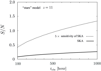
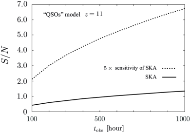
Figure 5: The $S/N$ ratio for the detection of the cross-correlation signal at $z=11$ as a function of the observation time. The left panel is for the “stars” model and the right panel is for the “QSOs” model. In both panels, the solid and dotted lines represent $S/N$ for SKA and for the observation with a 5 times better sensitivity than that of SKA, respectively. We set $f_{\rm sky}\sim 0.02$ in all plots.

5 conclusion

We investigated the small scale cross-correlation between CMB anisotropies and the 21 cm fluctuations during the EoR in harmonic space. The CMB anisotropies at small scales are mainly caused by the kSZ effect which is the second order fluctuation effect generated by the peculiar velocity and the fluctuations of the visibility function. We therefore calculated the cross-correlation with the second order fluctuations of 21 cm fluctuations.

The cross-correlation signal between kSZ and 21 cm fluctuations is negative on small scales. This anti-correlation on small scales was found in the numerical simulations of Salvaterra et al. (2005) and Jelić et al. (2010). We found that the position of the negative peak is at the angular scale corresponding to the typical size of an ionised bubble at the redshift probed by 21 cm fluctuation measurements. This angular scale shifts to larger scales as ionised bubbles evolve. The amplitude also increases with the reionisation process until the average ionisation fraction reaches $\bar{x}_{i}\sim 0.9$. The amplitude of the cross-correlation strongly depends on the typical bubble size. The cross-correlation in the case of larger bubbles has a higher amplitude than in the case of smaller bubbles, even if in both cases the mean ionisation fractions are the same. Moreover, the amplitude of the cross-correlation from large ionised bubbles is comparable to that of the first order cross-correlation. Those characteristic features of the cross-correlation could be used to distinguish between different reionisation histories with future observations.

We also estimated the detectability of the small-scale cross-correlation by the current design sensitivity of SKA. It is rather difficult to detect the cross-correlation signal even in the radical reionisation cases. However, if the sensitivity is improved by a factor of 5, the detection or non-detection of the cross-correlation signal will definitely provide information about the EoR.