Improved Scaling for Quantum Monte Carlo on Insulators

Abstract

Quantum Monte Carlo (QMC) methods are often used to calculate properties of many body quantum systems. The main cost of many QMC methods, for example the variational Monte Carlo (VMC) method, is in constructing a sequence of Slater matrices and computing the ratios of determinants for successive Slater matrices. Recent work has improved the scaling of constructing Slater matrices for insulators so that the cost of constructing Slater matrices in these systems is now linear in the number of particles, whereas computing determinant ratios remains cubic in the number of particles. With the long term aim of simulating much larger systems, we improve the scaling of computing the determinant ratios in the VMC method for simulating insulators by using preconditioned iterative solvers.

The main contribution of this paper is the development of a method to efficiently compute for the Slater matrices a sequence of preconditioners that make the iterative solver converge rapidly. This involves cheap preconditioner updates, an effective reordering strategy, and a cheap method to monitor instability of ILUTP preconditioners. Using the resulting preconditioned iterative solvers to compute determinant ratios of consecutive Slater matrices reduces the scaling of QMC algorithms from $O(n^{3})$ per sweep to roughly $O(n^{2})$, where $n$ is the number of particles, and a sweep is a sequence of $n$ steps, each attempting to move a distinct particle. We demonstrate experimentally that we can achieve the improved scaling without increasing statistical errors. Our results show that preconditioned iterative solvers can dramatically reduce the cost of VMC for large(r) systems.

1 Introduction

Quantum Monte Carlo (QMC) methods [33, 23], like the Variational Monte Carlo method (VMC), produce highly accurate quantitative results for many body systems. They have a wide range of applications, including the study of the electronic structure of helium, molecules, solids, and lattice models. The QMC method is computationally expensive, and current algorithms and computers limit typical system sizes for fermionic systems to about a thousand particles [19, 27, 32]. There are two main bottlenecks to simulating larger systems. The first is constructing a sequence of millions of so-called Slater matrices, and the second is computing the ratios of determinants of successive Slater matrices. We will briefly describe VMC, Slater matrices, and other relevant concepts in section 2, but first we discuss the scaling of these bottlenecks. Our longer term aim is to develop methods for the efficient simulation of systems with $10^{4}$ to $10^{5}$ particles (on high-end computers).

Let $n$, the system size, be the number of particles (electrons) in the system, which also equals the number of orbitals. Each orbital is a single particle wave function. For simplicity we ignore spin; incorporation of spin is straightforward. In VMC, we estimate observables by conditionally moving particles one by one and accumulating ‘snapshots’ of the observables; see section 2. We define the attempt to move all the particles in the system once as a sweep. The cost of constructing Slater matrices depends on the type of basis functions used for building the orbitals. We discuss this dependency in the next section; however, the cost for the generic case is $O(n^{2})$ per sweep [35] (constant cost per element in the matrix). Recent physics papers [3, 2, 35] discuss methods to reduce this cost to $O(n)$ by optimizing the orbitals, such that the matrix is optimally sparse. Therefore only a linear number of elements in the matrix must be filled and computing the matrix becomes cheap. This can only be shown to be rigorous for certain physical systems (like insulators). These methods are referred to as ‘linear scaling’ or ‘O(n)’ methods, because, in many cases, the cost of computing the Slater matrices dominates. However, these methods are not truly linear, since the cost of computing the determinant ratios is still $O(n^{3})$, which will dominate the cost of the VMC method for larger $n$. In this paper, we focus on reducing this cost for insulators (or, more generally, for systems with sparse Slater matrices) to $O(n^{2})$.

The VMC method generates a sequence of matrices,

$$A_{k+1} = A_{k}+e_{i_{k}}u_{k}^{T},$$ (1)

where $k$ indicates the Monte Carlo step or particle move, $A_{k}$ and $A_{k+1}$ are the Slater matrices before and after the proposed move of particle $i_{k}$, $e_{i_{k}}$ is the corresponding Cartesian basis vector, and $u_{k}$ gives the change in row $i_{k}$ resulting from moving particle $i_{k}$. The acceptance probability of the (conditional) move depends on the squared absolute value of the determinant ratio of the two matrices,

$$\frac{|\det A_{k+1}|^{2}}{|\det A_{k}|^{2}}=\left|1+u_{k}^{T}A_{k}^{-1}e_{i_{k}}\right|^{2}.$$ (2)

The standard algorithm in VMC [12] uses the explicit inverse of the Slater matrix, $A_{k}^{-1}$, to compute this ratio, and it updates this inverse according to the Sherman-Morrison formula [21, p. 50] if the particle move is accepted, resulting in $O(n^{3})$ work per sweep. For stability, the inverse is occasionally recomputed from scratch (but such that it does not impact the overall scaling). For systems with fewer than a thousand particles this method is practical. Recently, in [28] a variant of this algorithm was proposed that accumulates the multiplicative updates to the exact inverse,

$$A_{k+1}^{-1}=(I-\frac{1}{1+u_{k}^{T}A_{k}^{-1}e_{i_{k}}}A_{k}^{-1}e_{i_{k}}u_{k}^{T})A_{k}^{-1},$$

and applies those recursively to compute the ratio (2), an approach well-known in numerical optimization for Broyden-type methods [25, p. 88]. The same idea is also discussed in [5, Appendix A]. This approach requires $O(kn)$ work for the $k^{th}$ Monte Carlo step, and therefore $O(k^{2}n)$ work for the first $k$ Monte Carlo steps. Hence, a single sweep ($n$ Monte Carlo steps) takes $O(n^{3})$ work. If the inverse is not recomputed once per sweep, the approach will actually scale worse than the standard algorithm. So, this method does not decrease the total number of required operations (or scaling), but often has superior cache performance resulting in an increase in speed.

In this paper, we propose an algorithm for computing determinant ratios for insulating systems in the VMC method with roughly $O(n^{2})$ work per sweep, providing a significant improvement in the order of complexity over the standard algorithm; see the discussion of complexity and tables 4 and 5 in section 4.

Rather than keeping and updating the inverse of the Slater matrices, we can compute (2) in step $k$ by solving $A_{k}z_{k}=e_{i_{k}}$ and taking the inner product of $z_{k}$ with $u_{k}$. Since, for certain cases (like insulators), the Slater matrices with optimized orbitals are sparse, and the relative sparsity increases with the number of particles and nuclei in a system for a given material, preconditioned iterative methods are advantageous, especially since the accuracy of the linear solve can be modest. As we will show, convergence is rapid with a good preconditioner, and hence we use preconditioned full GMRES [31]. However, other Krylov methods are equally possible and might be more appropriate for harder problems. The main challenge in our approach is to generate, at low cost, a sequence of preconditioners corresponding to the Slater matrices that result in the efficient iterative solution of each system. We explain how to resolve this problem in section 3.

In section 2, we briefly discuss the VMC method. We discuss the efficient computation of a sequence of preconditioners and their use in computing determinant ratios by iterative solves in section 3. Section 4 gives numerical results that demonstrate experimentally the efficiency and favorable scaling of our approach. We also show that our approach works in practice. Finally, we discuss conclusions and future work in section 5.

2 The Variational Monte Carlo Method

The VMC method for computing the ground-state expectation value of the energy combines variational optimization with the Monte Carlo algorithm to evaluate the energy and possibly other observables [19, 33]. VMC is one of many forms of quantum Monte Carlo. Although our focus will be on variational Monte Carlo, our results naturally transfer to diffusion Monte Carlo methods [19] as well.

The inner loop of VMC involves sampling over configurations $R$ with the probability density $|\Psi_{\alpha}(R)|^{2}$ induced by the many body trial wave function $\Psi_{\alpha}(R)$ [33]. Here, $\alpha$ denotes the vector of variational parameters over which we minimize, and $R$ is a $3n$-dimensional vector representing the coordinates of all the particles in the system. This sampling is done using a Markov Chain Monte Carlo approach. For each independent configuration $R$ generated from the Markov Chain, observables ${\cal O}(R,\Psi_{\alpha})$ are computed and averaged. Although there are many possible observables, our discussion will focus on the the local energy, $E_{L,\alpha}$. The average of $E_{L,\alpha}$ is the function being optimized in the outer loop and consequently essential for any VMC calculation. In the rest of this section, we will further detail the separate pieces of this process with a particular focus on the computational bottlenecks.

2.1 Many Body Wave Function

Although wave functions come in a variety of forms, the most common form is

$$\Psi_{\alpha}(r_{1},r_{2},...,r_{n}) = \exp\left(\sum_{ij}f(r_{i}-r_{j})\right)\det(A),\quad\mbox{ with }$$ (3)

$$A = \left(\begin{array}[]{cccc}\phi_{1}(r_{1})&\phi_{2}(r_{1})&\ldots&\phi_{n}(r_{1})\\ \phi_{1}(r_{2})&\phi_{2}(r_{2})&\ldots&\phi_{n}(r_{2})\\ \vdots&&\ddots&\vdots\\ \phi_{1}(r_{n})&\phi_{2}(r_{n})&\ldots&\phi_{n}(r_{n})\end{array}\right),$$ (8)

where $f$ is called the Jastrow factor [12][33, p. 319], $r_{i}$ represents the coordinates of particle $i$ (part of the vector $R$), $A$ is called a Slater matrix (with elements $a_{i,j}=\phi_{j}(r_{i})$), and its determinant is called a Slater determinant. Each function $\phi_{j}$ is a scalar function of position and is referred to as a single particle orbital or single particle wave function. The calculation optimizes over these single particle orbitals as functions of the parameter vector $\alpha$. In this paper, we assume that the particles are confined to a cube and periodic boundary conditions are used.

The nature of the single particle orbitals depends on the physical system being simulated. (Since the determinants of the Slater matrices are invariant, up to the sign, under unitary transformations, we can only talk about properties of the set of orbitals.) Two important general classes of electronic systems are metals and insulators. In a metal, the single particle orbitals extend throughout all of space; there is no unitary transformation such that each orbital will have compact support. Moreover, forcing compact support by maximally localizing the orbitals and truncating them outside a fixed sphere can induce serious qualitative errors, e.g., changing the system from a metal to an insulator. In contrast, for an insulator there exists a choice of single particle orbitals that has compact support over small regions of space (or truncating them to introduce such local support produces minimal errors). As the size of the system is made large, the spread of the individual orbitals remains fixed, which leads to increasingly sparse matrices.

Previous work [2, 3, 35] has developed methods to find unitary transformations that minimize the spread of the single particle orbitals. These methods often go by the name linear scaling methods, although in practice they simply minimize the number of non-zero elements in the Slater matrix. Although this makes computing and updating the Slater matrix cheaper, the determinant computation still scales as $O(n^{3})$. Nonetheless, this is an important advance, which means that, for an insulating system, the Slater matrix can be made sparse. In this work, we focus on insulators and we leverage this starting point in our work with the assumption that our single particle orbitals are maximally localized.

The specific details of the single particle wave functions depend sensitively on the exact material being simulated and are unimportant for our study. Instead, we use a set of Gaussians centered on $n$ points tiled in space on a b.c.c. (body centered cubic) lattice as representative insulator single particle orbitals:

$$\phi_{j}(\textbf{r})=e^{-k\|\textbf{r}-\textbf{Z}_{j}\|^{2}},\quad\mbox{for }j=1\ldots n,$$ (9)

where the $\textbf{Z}_{j}$ are the lattice positions (i.e., physically the position of nucleus $j$), and $k$ determines the rate of decay of $\phi_{j}$. We will truncate these Gaussian functions so that they vanish outside some fixed radius (see section 4). These single particle orbitals have the same qualitative features as realistic single particle orbitals for insulators, have nice analytical properties that allow for easier analysis, and a solution to this problem will almost certainly translate to generic insulators. These Gaussians have a tuning parameter $k$ that determines their (effective) width and physically the bandwidth of the insulator. For these studies, we focus on $k=1$. (We remind the reader that we do not take spin degrees of freedom into account; in realistic simulations, one would have separate determinants for spin up and spin down electrons.) Furthermore, we choose the unit of length such that the density of electrons is $3/(4\pi)$. This implies that the b.c.c. lattice spacing is $2.031$ and the nearest neighbor distance between lattice/orbital positions is $1.759$. In this case, the Slater matrices depend on three choices (parameters), first, the type of lattice defining the orbital/nuclei positions, second, the spacing of the lattice positions, and, third, the decay rate of the Gaussian orbitals defined by $k$. After fixing the type of lattice (body centered cubic), physically, only the spacing of the orbital centers relative to the decay of the Gaussians is relevant. Hence, for analyzing the dependence of matrix properties on the parameters below, we need only vary $k$.

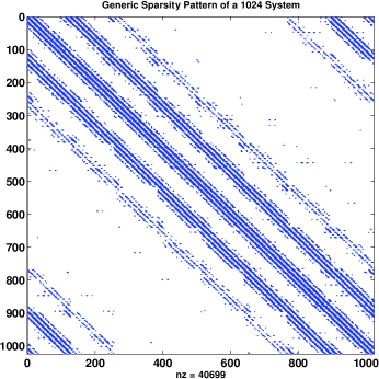
Fig. 1: Sparsity pattern for a typical configuration of our system for 1024 particles with $k=1$. For smaller $k$ the pattern remains more or less the same, while the number of nonzeros in the matrix increases. For larger $k$ the pattern also remains more or less the same, while the number of nonzeros in the matrix decreases.

Below, we provide a brief overview of properties of Slater matrices arising from the choices discussed above. First, in figure 1, we show the sparsity pattern of the Slater matrix for a typical configuration with $1024$ particles and $k=1$. As the basis functions have local support (after truncating outside a cut-off radius) and the electrons, on average, are distributed evenly, the sparsity pattern is similar to that of a finite difference matrix for a regular 3D grid and a relatively wide stencil, where the width of the stencil is comparable to the cut-off radius of the Gaussian orbitals (which in turn depends on $k$). Second, we give typical spectra for matrices arising from systems with $1024$ particles and $k=1.5$, $1$, and $0.5$. We point out that for the physics the ordering of rows and columns is irrelevant, since the square of the determinant is invariant under such changes. However, the eigenvalues can change significantly under reordering of rows and columns, which in turn can have a significant influence on the convergence of iterative methods (see section 3 for the reordering algorithm used). In figures 2–4, for each value of $k$, we provide the spectrum of a matrix before reordering, the spectrum of that same matrix after reordering, and the spectrum of that matrix after reordering and with preconditioning. The latter spectrum is the most relevant for the iterative solver.

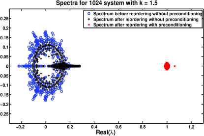
Fig. 2: Spectra for a typical configuration of our system for 1024 particles with $k=1.5$, before and after reordering, and with preconditioning for the reordered system.

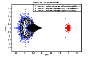
Fig. 3: Spectra for a typical configuration of our system for 1024 particles with $k=1$, before and after reordering, and with preconditioning for the reordered system. The value $k=1$ is used in the experiments reported in section 4.

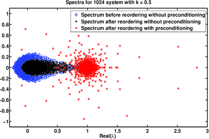
Fig. 4: Spectra for a typical configuration of our system for 1024 particles with $k=0.5$, before and after reordering, and with preconditioning for the reordered system. Note that the scale of this picture differs from the previous two. In addition, a lonely eigenvalue of the preconditioned system after reordering at $11.77$ has been left out to obtain a better scale.

Next, in Table 1, we provide typical condition numbers for various values of the parameter $k$ (in the Gaussian orbitals) and three problem sizes, $n=686$, $1024$, and $2000$. Note that, although for $k=0.5$ the condition number appears to increase slightly by preconditioning, the spectrum improves drastically. This also bears out in the iterative solver; preconditioning reduces the number of iterations. From Table 1, we see that the condition number of the unpreconditioned Slater matrix increases with decreasing $k$. This is to be expected; see, e.g., [9].

$k$	$1.5$			$1.0$			$0.5$
Size	686	1024	2000	686	1024	2000	686	1024	2000
$\kappa(A)$	73	1.4e2	1.3e3	1.6e2	6.7e2	6.7e2	2.4e3	1.1e4	8.3e3
$\kappa\left(A(LU)^{-1}\right)$	1.2	1.4	4.7	3.1	10	23	8.0e3	1.5e5	1.1e5

Table 1: Typical (spectral) condition numbers, $\kappa$, for Slater matrices and ILUTP preconditioned Slater matrices for $k=1.5$, $1$, $0.5$ and problem sizes $n=686$, $1024$, $2000$.

Although the orbitals for realistic systems (physical materials) may differ significantly from Gaussians, we expect many of the properties of the resulting Slater matrices to be similar. If orbitals decay sufficiently fast, the matrix will have the same banded sparsity pattern (after appropriate reordering) and be diagonally dominant or nearly so. In that case, all or most eigenvalues will be in the right half plane. However, a poor ordering of rows and columns will lead to eigenvalues located around the origin, as is the case here. If the decay is slow the matrix will become more ill-conditioned. Moreover, if the decay is sufficiently slow, there will be no ordering that yields diagonal dominance and the spectrum cannot be guaranteed to be in the right-half plane. In that case, we expect that there will be no ordering that, by itself, will lead to a nice spectrum (for iterative solvers), and preconditioning will be more important. Analyzing these properties and their dependency on the properties of orbitals, decay rate, and lattice type will be future work.

2.2 Markov Chain Monte Carlo

The Monte Carlo method is used to compute the high dimensional integrals of (10) below. Direct sampling would be very inefficient, because the wave function assumes large values only in a small region of the $3n$ dimensional space. Therefore, a Markov Chain Monte Carlo algorithm (MCMC) using a Metropolis update rule is used. For a comprehensive discussion of the Metropolis algorithm see [12, 19, 33]. The first VMC for bosonic systems was reported in [26].

The MCMC algorithm samples configurations as follows. At each step, the current configuration $R$ (representing the collective coordinates of all particles) is changed by moving one particle a small (random) distance, generating a trial configuration $R^{\prime}$. The particles can be moved in order or by random selection. The trial configuration is accepted with a probability that is equal to the ratio of the probabilities (densities) of the two configurations, assuming uniform sampling of the trial coordinate. Hence we compute $\frac{|\Psi(R^{\prime})|^{2}}{|\Psi(R)|^{2}}$ and compare with a random number drawn from the uniform distribution on $(0,1)$; the new configuration is accepted if the ratio is larger than the random number. Hence, this is where the determinant ratios arise. The exponentials of Jastrow factors must be computed as well, but since they are cheap for sufficiently large $n$ (in fact, they are identical in form to what is done in well-studied classical simulations [20, 4]), we will ignore them in this paper. If the trial configuration is accepted, the new configuration becomes $R^{\prime}$, otherwise the new configuration is $R$ (again). Since we move a single particle at each step, say particle $i$, in the trial configuration only $r_{i}$ is changed to $r^{\prime}_{i}$, and the Slater matrices (8) for the current configuration $R$ and the trial configuration $R^{\prime}$ differ only in row $i$. Therefore, consecutive Slater matrices in our MCMC algorithm differ in one row or are the same (when the trial configuration is rejected). We refer to the attempted move of one particle as a step and to the sequence of attempted moves of all particles as a sweep.

2.3 Local Energy

One important property of many body systems to calculate is the expectation value of the energy [19],

$$E_{V}=\frac{\int\Psi_{\alpha}^{*}(R)H\Psi_{\alpha}(R)dR}{\int\Psi_{\alpha}^{*}(R)\Psi_{\alpha}(R)dR}=\frac{\int|\Psi_{\alpha}(R)|^{2}E_{L,\alpha}(R)dR}{\int\Psi_{\alpha}^{*}(R)\Psi_{\alpha}(R)dR},$$ (10)

where $E_{L,\alpha}(R)=(H\Psi_{\alpha}(R))/\Psi_{\alpha}(R)$ is referred to as the local energy, and $H$ denotes the Hamiltonian of the system; see, for example, [33, section 4.5] and [23, p. 45]. Notice that the observable $E_{L,\alpha}(R)$ averaged over samples taken from the VMC sampling gives us the expectation value of the energy. The algorithm assumes that $\Psi_{\alpha}(R)$ and $\nabla\Psi_{\alpha}(R)$ are continuous in regions of finite potential. The computation of $E_{L,\alpha}(R)$ requires the calculation of the Laplacian $\nabla^{2}_{i}\Psi_{\alpha}(R)/\Psi_{\alpha}(R)$ and gradient $\nabla_{i}\Psi_{\alpha}(R)/\Psi_{\alpha}(R)$ with respect to each particle $i$. This must be done once per sweep. These quantities are computed by evaluating another determinant ratio. For a given $i$, we replace row $i$ in the Slater matrix by its Laplacian respectively its gradient, and then evaluate the ratio of the determinant of this matrix with the determinant of the Slater matrix. As this has to be done once per sweep, it also scales as $O(n^{3})$, and the methods described in this paper naturally generalize to evaluating these quantities by iterative methods with a reduced scaling.

As a point of note, the only computationally slow aspect of the Diffusion Monte Carlo method (DMC) that differs from VMC involves computing the gradient of the wave function for particle $i$ at each step where particle $i$ is moved. Again, the determinant ratio methods discussed in this paper are also applicable to this situation.

2.4 Optimization

The outer loop of the VMC method consists of updating the vector of variational parameters, $\alpha$, after the MCMC evaluation of the average of $E_{L,\alpha}$, so as to minimize the total average energy. In principle, these variational parameters could vary over all possible functions for all $n$ single particle orbitals. In practice, the orbitals are often optimized over a smaller subclass of possible functions. For example, in our model system, one might imagine optimizing $k$ or the location of the orbitals, $Z_{j}$ (i.e., off the b.c.c. lattice). In more realistic scenarios, each orbital itself has more structure and might be expanded in terms of basis functions such as plane waves or Gaussian basis functions (9). Often, then, the expansion factors will be optimized (in addition to the Jastrow factors). Care must be taken when using more complicated representations. If, for example, each single particle orbital is composed of $n$ plane waves and there are $n$ orbitals to be evaluated for $n$ particles, even constructing the Slater matrix would scale as $O(n^{3})$ per sweep. However, by tabulating the orbitals on a grid, and doing a table lookup when needed, the cost of constructing the matrix can be brought down to $O(n^{2})$ operations per sweep, since there are $O(n^{2})$ matrix elements, or $O(n)$ if the matrix is sparse.

In the next section, we describe our algorithm, which reduces the cost of evaluating determinant ratios for physically realistic systems to about $O(n^{2})$ per sweep.

3 Algorithmic Improvements

As described in the previous section, the sequence of particle updates, moving particle $i_{k}$ at step $k$ in the MCMC method, leads to a sequence of matrix updates for the trial configuration,

$$\tilde{A}_{k}=A_{k}+e_{i_{k}}u_{k}^{T}=A_{k}(I+A_{k}^{-1}e_{i_{k}}u_{k}^{T}),$$ (11)

where

$$(u_{k})_{j}=\phi_{j}(r^{\prime}_{i_{k}})-\phi_{j}(r_{i_{k}}),\quad\mbox{ for }j=1,\ldots,n,$$ (12)

$A_{k}$ is the Slater matrix at the ${k}^{th}$ Monte Carlo step, $e_{i_{k}}$ is the Cartesian basis vector with a $1$ at position $i_{k}$, the $\phi_{j}$ are the single particle orbitals used in (3)–(8), and $r_{i_{k}}$ and $r^{\prime}_{i_{k}}$ are the old and the new position of the particle $i_{k}$, respectively. We do not need to compute $\phi_{j}(r_{i_{k}})$ since it equals $(A_{k})_{i_{k},j}$. The acceptance probability of the trial configuration depends on the squared absolute value of the determinant ratio of the two matrices,

$$\frac{|\det\tilde{A}_{k}|^{2}}{|\det A_{k}|^{2}}=\left|1+u_{k}^{T}A_{k}^{-1}e_{i_{k}}\right|^{2},$$ (13)

which can be computed by solving the linear system $A_{k}z_{k}=e_{i_{k}}$ and taking the inner product $u_{k}^{T}z_{k}$. We compare the value from (13) with a random number drawn from the uniform distribution on $(0,1)$. If the trial configuration giving $\tilde{A}_{k}$ is accepted, $A_{k+1}=\tilde{A}_{k}$, if the trial configuration is rejected, $A_{k+1}=A_{k}$.

The use of maximally localized single particle orbitals leads to a sparse Slater matrix in some cases (insulators). In this case, iterative solvers provide a promising approach to compute these determinant ratios, as long as effective preconditioners can be computed or updated cheaply. Variations of incomplete decompositions (such as incomplete LU) are good candidates for this problem, as they have proven effective for a range of problems and require no special underlying structure (in principle). Unfortunately, the sequence of particle updates leads to matrices that are far from diagonally dominant, often have eigenvalues surrounding the origin, and have unstable incomplete decompositions in the sense defined in [6, 30]. However, the properties of orbitals and localization suggest that with a proper ordering of orbitals and particles the Slater matrix will be nearly diagonally dominant. Our method resolves the preconditioning problem by combining the following three improvements.

First, we have derived a geometric reordering of electrons and orbitals, related to the ordering proposed in [18], that provides nearly diagonally dominant Slater matrices. This ordering combined with an ILUTP preconditioner [29, 30] leads to very effective preconditioners; see section 4. However, reordering the matrix and computing an ILUTP preconditioner every (accepted) VMC step would be too expensive. Therefore, as the second improvement, we exploit the fact that $A_{k+1}=A_{k}(I+A_{k}^{-1}e_{i_{k}}u_{k}^{T})$ (11) and use a corresponding update to the right preconditioner, $M_{k}$, such that $A_{k+1}M_{k+1}=A_{k}M_{k}$. This leads to cheap intermediate updates to our preconditioners. Moreover, if $M_{k}$ has been computed such that $A_{k}M_{k}$ has a favorable spectrum for rapid convergence [34, 22, 30], then subsequent preconditioned matrices, $A_{k+s}M_{k+s}$, have the same favorable spectrum. However, each update increases the cost of applying the preconditioner, and we periodically compute a new ILUTP preconditioner. Third, we assess whether potential instability of the incomplete LU decomposition affects the iteration by applying the stability metrics from [6, 30, 14] in an efficient manner. We only reorder the matrix if instability occurs, or if our iterative solver does not converge to the required tolerance in the maximum number of iterations, or if our iterative solvers takes more than four times the average number of iterations. This monitoring and reordering is necessary as the matrix becomes far from diagonally dominant and the incomplete LU decompositions slowly deteriorate due to the continual updates to the Slater matrix. This approach has proved very effective and limits the number of reorderings to a few per sweep. In spite of the matrix reordering, the explicit reordering of electrons and orbitals, based on the stability metric discussed below or on slow convergence, pivoting in the incomplete LU factorization is necessary. If we do not pivot the factorization occasionally breaks down. Such a breakdown could be avoided by doing the explicit reordering of electrons and orbitals every step, but this would be too expensive. Moreover, not pivoting leads to denser $L$ and $U$ factors and slower convergence in the iterative linear solver; both effects increase the total amount of work.

3.1 Reordering for Near Diagonal Dominance and Efficient Reordering Criteria

First, we discuss an efficient way to judge the quality of the preconditioner. In the second part of this section, we discuss a reordering that improves the quality of the preconditioner.

The quality of an ILU preconditioner for the matrix $A$, $LU\approx A$, can be assessed by its accuracy and stability [6]. The accuracy of the ILU preconditioner, defined as

$$N_{1}=||A-LU||_{F},$$ (14)

measures how close the product $LU$ is to the matrix $A$. The stability of the preconditioner, for right preconditioning defined as

$$N_{2}=||I-A(LU)^{-1}||_{F},$$ (15)

measures how close the preconditioned matrix is to the identity. For left preconditioning, $N_{2}=||I-(LU)^{-1}A||_{F}$. Although for some classes of matrices $N_{1}$ is a good measure of preconditioning quality, for general matrices $N_{2}$ is a more useful indicator [6, 7]. We will see that this is also the case here. In general, instability arises from a lack of diagonal dominance and manifests itself in very small pivots and/or unstable triangular solves.

In practice, computing $N_{2}$ is much too expensive, and we need to consider a more economic indicator. An alternative approach, suggested in [14], is to compute $||(LU)^{-1}e||_{\infty}$, where $e$ is the vector of all $1$’s. However, this still requires solving an additional linear system. Instead, we propose to use an effective or local stability measure,

$$N=\max_{i}\|v_{i}-A(LU)^{-1}v_{i}\|_{2},$$ (16)

where the $v_{i}$ are the Arnoldi vectors generated in the GMRES algorithm [31] during a linear solve. $N$ measures the instability of the preconditioned matrix over the Krylov space from which we compute a solution. If $N$ is small, there is no unit vector $z\in K_{m}(A(LU)^{-1},r_{0})$ for which $\|(I-A(LU)^{-1})z\|_{2}$ is large (where $m$ is the number of GMRES iterations). Indeed, for unit $z\in K_{m}(A(LU)^{-1},r_{0})$, $\|(I-A(LU)^{-1})z\|_{2}\leq mN$. $N$ can be small or modest when $N_{2}$ is large; however, this indicates that the instability does not play a role for vectors in the subspace over which a solution was computed; hence, the name effective or local stability. Note that $N$ can be computed during the GMRES iteration at negligible cost, in contrast to the expensive computation of $N_{2}$. If $N$ is large, the preconditioned matrix is ill-conditioned over the Krylov space used to find a solution, and we reorder the matrix as described below. Large $N$ indicates that the solution might be inaccurate and that the preconditioner is deteriorating. This typically would lead to poor convergence either in the present solve or later, and so reordering and updating the preconditioner is better.

To check whether $N_{1}$ and $N_{2}$ are good indicators of preconditioner quality for our problem, we run the MCMC algorithm for $100$ sweeps for a test problem with $2000$ particles, and we check $N_{1}$ and $N_{2}$ each time GMRES does not converge in $15$ iterations (which is relatively slow; see section 4). It would be useful to check the reverse as well, but computing $N_{1}$ and $N_{2}$ for every MC step ($200,000$ steps) would be too expensive. If GMRES does not converge in $15$ iterations, we reorder the matrix as described below, compute a new ILUTP preconditioner, and solve the linear system again from scratch. This procedure always led to convergence within $15$ iterations after the reordering. Although the experiments in section 4 are computed using a C/C++ code, for experiments in this subsection we use a Matlab based VMC code, developed for easy experimentation, that uses the GMRES and luinc routines of Matlab. The code uses left preconditioning, luinc with a drop tolerance of $\tau=0.01$, and it allows pivoting in the entire pivot column (default). Furthermore, we use Gaussian orbitals (9) with $k=1$.

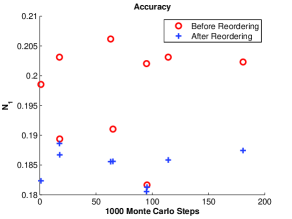
Fig. 5: Accuracy before and after reordering.

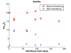
Fig. 6: Stability before and after reordering.

In Figures 5 and 6 we plot, respectively, $N_{1}$ and $N_{2}$ at those Monte Carlo steps where the GMRES algorithm does not converge in $15$ iterations, implying a deterioration of the preconditioner. We also plot $N_{1}$ and $N_{2}$ after reordering and recomputing the preconditioner. Figure 5 shows that the accuracy is always quite good, and hence accuracy is not a good indicator for reordering the matrix to improve preconditioner quality. This is in line with observations from [6]. Reordering does improve the accuracy further. Figure 6 shows that poor convergence goes together with very large values of $N_{2}$, and so $N_{2}$ is a better indicator for reordering the matrix to improve the preconditioner. Note that reordering improves the stability significantly, and usually reduces it to modest values, but with some exceptions. As $N_{2}$ seems a good indicator, but too expensive, we next consider the effective stability $N$.

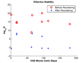
Fig. 7: Effective stability before and after reordering.

Figure 7 shows large values of $N$ corresponding to steps where the GMRES algorithm does not converge. The value of $N$ is modest at other Monte Carlo steps (note that it is easy to compute $N$ at every step). This demonstrates that $N$ is an equally good indicator of the effectiveness of the preconditioner as $N_{2}$, and hence we will use $N$ as an indicator for matrix reordering. We remark that more timely reordering (before $N$ gets so large that the matrix is numerically singular) also leads to smaller values for $N$ after reordering the matrix and recomputing the preconditioner. Next, we discuss reordering the matrix when the quality of the preconditioner deteriorates.

Instability in the incomplete factorization, as discussed above (small pivots and/or ill-conditioned triangular solves), is generally associated with a lack of diagonal dominance [14, 6]. Instability can generally be removed or significantly reduced by preprocessing the coefficient matrix. Preprocessing strategies involve permutations and scalings for improving the conditioning, near-diagonal dominance, and the structure of the coefficient matrix; modifications such as perturbing diagonal elements are also possible [14, 6]. Improving near-diagonal dominance of the matrix through a judicious ordering of unknowns and equations has been shown quite effective in addressing instability, leading to a better preconditioner. In [7], the authors show that a simple reordering of the matrix can improve the quality of incomplete factorization preconditioners. More sophisticated reorderings that improve the near-diagonal dominance of the matrix are discussed in [16, 17]. These papers also show that reordering can have a dramatic effect on the convergence of ILU preconditioned iterative methods. Reorderings that exploit the physics of the underlying problem have also proved quite effective [13].

We remark that the physics underlying our problem and the optimization of orbitals suggest that a proper ordering should lead to a nearly diagonally-dominant matrix. We also observe that, as all orbitals are scaled equally, we do not expect scaling to provide much improvement.

Since the orbitals used in our study are monotonically decreasing with distance, we propose a reordering that is simple, improves the near-diagonal dominance of the Slater matrix, and incorporates the physics of our problem. This reordering strategy performs a geometric reordering of particles and orbitals, and is similar to the reordering of inputs and outputs for a reliable control scheme in [18]. Our algorithm consists of the following steps, ignoring sparsity for simplicity.

1.	Label the particles ($P_{i}$) and orbitals ($O_{j}$) from $1$ to $n$,
	giving the following Slater matrix $A$:
	$\displaystyle\hbox{}\;\vbox{\kern 48.63776pt\hbox{$\kern 128.29214pt\kern-8.75pt\left(\kern-128.29214pt\vbox{\kern-48.63776pt\vbox{\halign{$#$\hfil\kern 2\p@\kern\@tempdima& \thinspace\hfil$#$\hfil&& \quad\hfil$#$\hfil\cr\hfil\crcr\kern-12.0pt\cr$\hfil\kern 2.0pt\kern 8.75pt&O_{1}&O_{2}&&O_{n}\crcr\kern 2.0pt\cr P_{1}$\hfil\kern 2.0pt\kern 8.75pt&\phi_{1}(r_{1})&\phi_{2}(r_{1})&\cdots&\phi_{n}(r_{1})\cr P_{2}$\hfil\kern 2.0pt\kern 8.75pt&\phi_{1}(r_{2})&\phi_{2}(r_{2})&\cdots&\phi_{n}(r_{2})\cr$\hfil\kern 2.0pt\kern 8.75pt&\vdots&\vdots&&\vdots\cr P_{n}$\hfil\kern 2.0pt\kern 8.75pt&\phi_{1}(r_{n})&\phi_{2}(r_{n})&\cdots&\phi_{n}(r_{n})\cr\cr}}\kern-12.0pt}\,\right)$}},$
2.	for $i=1$, …, $n-1$ do
		Find the closest orbital $O_{j}$ to $P_{i}$ for $j\in\{i,i+1,\ldots,n\}$
		if $j\neq i$ then
			renumber $O_{j}$ as $O_{i}$ and $O_{i}$ as $O_{j}$ (swap columns $j$ and $i$)
		else
			find the particle $P_{k}$ closest to orbital $O_{i}$ for $k\in\{i,i+1,\ldots,n\}$
			if $k\neq i$ then
				renumber $P_{k}$ as $P_{i}$ and $P_{i}$ as $P_{k}$ (swap rows $i$ and $k$)
			end if
		end if
	end for

As mentioned above, reordering the matrix and recomputing the ILUTP preconditioner always leads to convergence within $15$ GMRES iterations. So, the algorithm is quite effective. We can see from Figure 7 that $N$ is always significantly reduced by reordering the matrix and recomputing the preconditioner. Moreover, more timely reordering of the matrix, before $N$ gets so large that the matrix is numerically singular, also leads to smaller values for $N$ after reordering.

The computational cost of a straightforward implementation of this reordering is $O(n^{2})$. Since for our current experiments (and problem sizes) the runtime of reordering is negligible and reordering is needed only two or three times per sweep, we have not (yet) focused on an efficient implementation, especially since this likely requires substantial work in the software for matrix storage and manipulation. However, we will do this in the future. We remark that for sparse matrices where the number of nonzeros per row and per column is roughly constant, independent of $n$, an $O(n)$ implementation is possible. Moreover, this global reordering algorithm ignores the local nature of the particle updates and resulting changes to the matrix. In addition, maintaining further (multilevel) geometric information related to relative positions of particles and orbitals should make reordering more efficient. Hence, longer term we expect to replace this algorithm by one that makes incremental updates to the local ordering. If we start with a good ordering and the matrix is sparse (in the sense that the decay of the orbitals does not depend on the problem size), we expect that such local updates can be done at constant or near constant cost.

3.2 Cheap Intermediate Updates to the Preconditioner

Computing a new ILUTP preconditioner for every accepted particle update would be very expensive. However, we can exploit the structure of the matrix update to compute a cheap update to the preconditioner that maintains good convergence properties.

Assume that at some step $k$ we have computed an incomplete LU preconditioner (ILU) with threshold and pivoting from the matrix $A_{k}$. We have

$$A_{k}Q_{k}\simeq L_{k}U_{k},$$ (17)

where $Q_{k}$ is a column permutation matrix, and $L_{k}$ and $U_{k}$ are the incomplete lower and upper triangular factors, respectively. We consider right preconditioning, and so, instead of $A_{k}z_{k}=e_{i_{k}}$, we solve the right preconditioned linear system,

$$A_{k}M_{k}\tilde{z}_{k}=e_{i_{k}}\quad\mbox{with}\quad z_{k}=M_{k}\tilde{z}_{k},$$ (18)

where $M_{k}=Q_{k}\left(L_{k}U_{k}\right)^{-1}$ is the preconditioner. If the trial move of particle $i_{k}$ is accepted, we consider for the next step the updated matrix $A_{k+1}=A_{k}(I+(A_{k}^{-1}e_{i_{k}})u_{k}^{T})$; see (11). Now, let $M_{k}$ be such that $A_{k}M_{k}$ has a favorable spectrum for rapid convergence [34, 22, 30]. Then defining the updated preconditioner $M_{k+1}$ such that $A_{k+1}M_{k+1}=A_{k}M_{k}$ gives a new preconditioned matrix with the same favorable spectrum. Hence, we define the new preconditioner as

$$M_{k+1}=(I+(A_{k}^{-1}e_{i_{k}})u_{k}^{T})^{-1}M_{k}=\left(I-\frac{(A_{k}^{-1}e_{i_{k}})u_{k}^{T}}{1+u_{k}^{T}A_{k}^{-1}e_{i_{k}}}\right)M_{k},$$ (19)

without explicitly computing $M_{k+1}$. Since $A_{k}^{-1}e_{i_{k}}=z_{k}$ and $1+u_{k}^{T}A_{k}^{-1}e_{i_{k}}$ have already been computed to find the determinant ratio (13), we get $M_{k+1}$ for free, and the cost of applying $M_{k+1}$ is that of applying $M_{k}$ plus the cost of a dot product and vector update. Let $\hat{z}_{k}=(1+u_{k}^{T}A_{k}^{-1}e_{i_{k}})^{-1}z_{k}$. Then $M_{k+1}$ is defined as

$$M_{k+1} = (I-\hat{z}_{k}u_{k}^{T})Q_{k}(L_{k}U_{k})^{-1},$$ (20)

where the inverse of $L_{k}U_{k}$ is implemented, of course, by a forward solve for $L_{k}$ and a backward solve for $U_{k}$.

Since $z_{k}$ is approximated by an iterative process, and there is no need to solve very accurately, we have $A_{k+1}M_{k+1}\approx A_{k}M_{k}$, rather than exact equality. However, we have the following result. Let $\zeta_{k}=A_{k}^{-1}e_{i_{k}}$ and let $r_{k}=e_{i_{k}}-A_{k}z_{k}=A_{k}(\zeta_{k}-z_{k})$. Then we have

$$A_{k+1}M_{k+1} = A_{k}(I+\zeta_{k}u_{k}^{T})(I-\frac{z_{k}u_{k}^{T}}{1+u_{k}^{T}z_{k}})M_{k}$$

$$= A_{k}\left(I+\zeta_{k}u_{k}^{T}-\frac{\zeta_{k}u_{k}^{T}}{1+u_{k}^{T}z_{k}}+\frac{(\zeta_{k}-z_{k})u_{k}^{T}}{1+u_{k}^{T}z_{k}}-\zeta_{k}u_{k}^{T}\frac{u_{k}^{T}z_{k}}{1+u_{k}^{T}z_{k}}\right)M_{k}$$

$$= A_{k}\left(I+\frac{(\zeta_{k}-z_{k})u_{k}^{T}}{1+u_{k}^{T}z_{k}}\right)M_{k}$$

$$= A_{k}M_{k}+\frac{r_{k}u_{k}^{T}}{1+u_{k}^{T}z_{k}}M_{k}.$$

So, the relative change in the preconditioned matrix is small unless $|1+u_{k}^{T}z_{k}|$ is very small or $\|r_{k}\|\|M_{k}\|$ is large relative to $\|A_{k}M_{k}\|$. However, $|1+u_{k}^{T}z_{k}|$ governs the acceptance probability of the particle move. So, a very small value would occur in the preconditioner update with very small probability; we do not need to update the preconditioner if a trial move is rejected. This also guarantees that an accepted particle move will never result in a singular matrix, as the move will be accepted with probability $0$. If $\|M_{k}\|$ is large while $\|A_{k}M_{k}\|$ is small (say $O(1)$), then $A$ must have small singular values. In that case, an accurate $z_{k}$ requires a sufficiently small residual. Hence, unless $\|A_{k}M_{k}\|$ is large (which monitoring $N$ guards against), a proper choice of stopping criterion for $\|r_{k}\|$ should keep the relative change in the preconditioned matrix small.

Obviously, we can repeat the update of the preconditioner for multiple updates to the matrix. Defining $z_{s}=A_{s}^{-1}e_{i_{s}}$ (approximately from the iterative solve) and $\hat{z}_{s}=(1+u_{s}^{T}z_{s})^{-1}z_{s}$, where $u_{s}$ is given by (12) and $s=k,\ldots,k+m$, we have

$$M_{k+m} = \left(I-\hat{z}_{k+m-1}u_{k+m-1}^{T}\right)\cdots\left(I-\hat{z}_{k+1}u_{k+1}^{T}\right)\left(I-\hat{z}_{k}u_{k}^{T}\right)M_{k}.$$ (21)

In this case, the cost of applying the preconditioner slowly increases, and we should compute a new ILUTP preconditioner when the additional cost of multiplying by the multiplicative updates exceeds the (expected) cost of computing a new preconditioner. Of course, we also must compute a new preconditioner if we reorder (large $N$).

This technique for updating the preconditioner is similar to the idea of updating the (exact) inverse of the Jacobian matrix for Broyden’s method [25], which is applied to the exact inverse of the Slater matrix in [28]. See also [8] which uses a similar approach to updating a preconditioner, however, for a general nonlinear iteration. So, the notion to keep the preconditioned matrix fixed, $A_{k+1}M_{k+1}=A_{k}M_{k}$, appears to be new.

4 Numerical Experiments

In this section, we numerically test our new algorithm. Apart from testing the performance of our algorithm, we must also test its reliability and accuracy. Since we compute the determinant ratios in the MCMC algorithm by iterative methods, we replace the acceptance/rejection test by an approximate test. In addition, the updating of preconditioners and their dependence on occasional reordering may lead to slight inconsistencies in the computed acceptance/rejection probabilities. This may affect the property of detailed balance for equilibrated configurations. Although we assume that using sufficiently small tolerances would make such potential problems negligible, we test and compare an observable (kinetic energy) computed in the new algorithm and in the standard algorithm. We remark that the standard method, with an updated inverse, also has the potential of accumulation of errors, which may affect its accuracy. However, the standard algorithm has performed satisfactorily, and a successful comparison of the results of our algorithm to those of the standard algorithm should engender confidence.

As described in section 2, we use Gaussian functions for the single-particle orbitals with $k=1$, and we ignore the Jastrow factor. The lattice (giving the approximate locations of the nuclei in a solid) is selected as a Body Centered Cubic (b.c.c.) lattice, a lattice formed by cubes with nuclei/orbitals on all vertices and one in the middle. To test the scaling of our method, we fix the density of the electrons at $(3/4\pi)=0.2387$ ptcl/unit and increase the number of electrons $n$; this corresponds to increasing the number of cubes in the lattice. This causes the number of orbitals to increase linearly with the electron number. As the orbitals are located on a b.c.c. lattice, we choose values of $n=2K^{3}$ where $K$ is an integer representing the number of orbitals along one side of the computational domain, and so the b.c.c. lattice is commensurate with the periodic box. Note that this leaves the spacing of the lattice (the distance between orbitals) the same for all $n$. The length of the side of a cube is $2.031$, and the nearest neighbor distance is $1.759$. The calculation of properties on larger and larger lattices is a typical procedure in QMC simulations to estimate the errors induced by not simulating an infinite number of particles. It is important to recognize that, although we are simulating an insulator, the electrons are not confined to the neighborhood of a single orbital and move around the entire box (hence the need for occasional reordering of the matrix). Since we use Gaussian orbitals, the Slater matrix has no coefficients that are (exactly) zero. However, most of the coefficients are very small and negligible in computations. Therefore, to make the matrix sparse, we drop entries less in absolute value than $10^{-5}$ times the maximum absolute value of any coefficient in the matrix. The number of non-zeros per row of the matrix varies between $40$ and $50$.

We use QMCPACK [24] for our simulations and, in its standard version, for comparison. In order to efficiently implement our iterative algorithms, we rewrote a significant part of QMCPACK to handle sparse matrices . It might be advantageous to work with sparse vectors as well (sometimes referred to as sparse-sparse iterations) as the right hand sides in (18) are Cartesian basis vectors. On the other hand, the preconditioner may quickly destroy sparsity of the iteration vectors. This remains something to test in the future. We integrated the new components of our VMC algorithm in QMCPACK [24] (written in C/C++); this includes the GMRES algorithm [31], the ILUTP preconditioner [29], our algorithms to update the preconditioner by rank-one updates to the identity (section 3.2), our reordering algorithm (section 3.1), and our test for instability of the preconditioner (section 3.1).

To simulate the system and gather statistics on the quality of the results for the new method and on its performance, we carry out $120$ sweeps. We discount the data corresponding to the first $20$ sweeps, which are used to ensure that the system is in equilibrium.

In the GMRES algorithm, we set the maximum number of iterations to $40$, and the relative convergence tolerance to $10^{-6}$. We monitor $N$, the effective stability (see section 3.1), to decide when to reorder the matrix; we reorder when $N>100$. This is relatively low, but from experience this leads to faster (average) convergence. Note that, in our experiments, the number of reorderings is never more than three per sweep (see below). Finally, since $N$ does not always predict slow convergence, even though it is quite reliable, we also reorder when the number of GMRES iterations reaches four times the average number of iterations or when the method does not converge in the maximum number of iterations. However, the occurrence of slow convergence while $N$ is small accounts only for a very small fraction of the total number of reorderings, a few percent at most. If $N>100$ or GMRES does not converge fast enough, we solve the same system again (from scratch) after reordering and computing a new preconditioner (GMRES is not restarted); this always resolves the convergence problem in our tests. In figures 8 and 9, we provide some information on $N$ for the system with $4394$ particles. In figure 8, we give $\log_{10}(N)$ for each Monte Carlo step in a representative window of roughly $6000$ MC steps (the number of reorderings in this window is slightly higher than average though); in figure 9, we provide a histogram for the number of Monte Carlo steps between reorderings (each bin is of size $100$). We note that sometimes reorderings follow each other with relatively short intervals. For the $4394$ system, we have on average $2.73$ reorderings per sweep (see table 4); so, the number of steps between reorderings is, on average, about $1600$ steps. However, we have a fair number of much shorter intervals. We conjecture that such shorter intervals occur when multiple particles are not relatively close to any orbital (nucleus), for example, when multiple pairs of electrons ‘swap’ nuclei. As the matrix changes only by one row per (successful) step and only by a modest amount, it is likely that matrices for which a good preconditioner is difficult to compute are clustered in the MCMC sequence. Alternatively, this phenomenon might suggest that we need a better reordering algorithm.

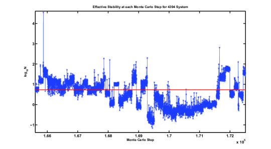
Fig. 8: Effective stability, $N$, at each Monte Carlo step for the $4394$ system for a representative window of roughly $6000$ steps. The horizontal (red) line indicates the ($\log_{10}$ of) the average $N$ (the average $N$ is around $5.36$).

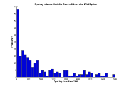
Fig. 9: Histogram for the number of steps between reorderings (large $N$ or slow convergence) for the $4394$ system. The size of each bin is $100$.

For preconditioning, we use the ILUTP preconditioner from SPARSKIT [30]. This preconditioner uses pivoting and a relative threshold to drop (off-diagonal) coefficients based on magnitude to obtain sparse lower triangular and upper triangular factors, $L$ and $U$, such that $AQ\approx LU$. We set the relative drop tolerance to $0.01$ and we allow pivoting in the entire row. We set the permutation tolerance that governs the pivoting to $0.05$. Finally, in ILUTP one can set the maximum number of additional nonzeros (fill-in) per row allowed in both the $L$ and $U$ factor. We set this to half the average number of nonzeros per row of the matrix, resulting in at most twice as many nonzeros in the $L$ and $U$ factor together as in the matrix, $A$. The average number of nonzeros in the preconditioner remains well below this maximum; see Table 4.

The experimental results are given in four tables. In the first two tables, we compare the results of our method to those of the standard method to demonstrate the reliability and accuracy of the new method. In the other two tables, we assess the scaling of our method as the number of particles increases.

First, we assess how close the determinant ratio computed by the new method is to that computed by the standard method. This determines the probability of a wrong decision in the acceptance/rejection test. Let $q$ be the exact determinant ratio squared and $q_{a}$ be the approximate determinant ratio squared computed by an iterative method; then the probability of a wrong decision at one step in the Metropolis algorithm is $f=|min(q,1)-min(q_{a},1)|$. The average value of $f$ over a random walk (the entire sequence of MCMC steps), $\bar{f}$, gives the expected number of errors in the acceptance/rejection test (Exp. Errors in Table 2). We call an approximation

• extremely good if $f<0.0001$,

• very good if $f<0.001$, and

• good if $f<0.01$.

The results of this test for eight successive problem sizes ($2\cdot 7^{3}$, $2\cdot 8^{3}$, …, $2\cdot 14^{3}$) are given in Table 2. The high percentage of extremely good approximations in Table 2 shows that approximating determinant ratios does not interfere with the accuracy and reliability of the simulation. In fact, the new algorithm makes a different accept/reject decision from that made by the standard algorithm only once every $10^{5}$ steps. Since the autocorrelation time is smaller than this by over an order of magnitude, the system should quickly forget about this ‘incorrect’ step. Note that given the tolerance in GMRES the step is not unlikely even in the standard algorithm. We also report the acceptance ratio, which is defined as the ratio of the number of accepts to the total number of Monte Carlo steps. The desired range of the acceptance ratio is between $0.2$ and $0.8$, and this is satisfied in our simulation. Higher or lower acceptance ratios are likely to create problems, as this typically indicates that successive MC steps remain correlated for a long time [10].

Size	686	1024	1458	2000	2662	3456	4394	5488
Exp. Errors	4.45e-6	4.22e-6	5.03e-6	4.41e-6	4.63e-6	4.50e-6	3.96e-6	4.07e-6
Extr. Good	99.49	99.53	99.57	99.49	99.50	99.47	99.56	99.56
Very Good	99.99	99.98	99.99	99.99	99.99	99.99	99.99	99.99
Good	100	100	100	100	100	100	100	100
Acc. Ratio	0.5879	0.5880	0.5887	0.5880	0.5881	0.5898	0.5878	0.5883

Table 2: Accuracy of the acceptance/rejection test, giving the average expected number of errors in the acceptance test (Exp. Errors), the percentage of extremely good approximations (Extr. Good), the percentage of very good approximations (Very Good), the percentage of good approximations (Good), and the acceptance ratio of trial moves (Acc. Ratio).

To further check the accuracy of the results of the simulation, we compute the kinetic energy of the system (an important observable). The kinetic energy of the system is defined as

$$E=\frac{\hbar^{2}}{2\rho n}\sum_{ij}\left(6k-4k^{2}||r_{j}-Z_{i}||^{2}\right)A_{ij}\left({A}^{-1}\right)_{ji},$$ (22)

where $\hbar$ is the reduced Planck’s constant ($h/2\pi$), $\rho$ is the electron mass, $n$ is the system size, $k=1$ is defined as in (9), $r_{j}$ is the position of particle $j$, $Z_{i}$ is the position of orbital $i$, and $A$ is the Slater matrix as given in (8). (We use units where $\hbar=\rho=1$). It should be noted that we use the exact kinetic energy in this test even though, in practice, our algorithm would also use iterative solvers to efficiently evaluate this observable (which involves the Laplacian of the wave function). This is done so as not to confound two sources of errors (one being a few rare ‘incorrect’ steps on the Markov chain and the other being errors in computing the kinetic energy). We compute the kinetic energy in two separate experiments. However, in order to emphasize how close the results of the new algorithm are to those of the standard algorithm, we start both experiments with the same starting configuration and using the same initial seed for the random number generator. Since the expectation of an incorrect acceptance/rejection is extremely small, both experiments follow the same chain for an extended period of time, and therefore the difference in kinetic energy between the experiments is much smaller than the statistical variation that would be expected if the chains were independent instead of correlated. We compute the kinetic energy by sampling (22) at the end of each sweep (doing $120$ sweeps and discarding the first $20$). The first experiment computes the determinant ratio for acceptance/rejection tests using the standard QMCPACK algorithm, while the second experiment uses the new (sparse) algorithm. The average energy over the whole simulation is listed in Table 3. It is evident that the energies from the two algorithms are close for all system sizes. We also compute the standard deviation of the kinetic energy, $\sigma$, using DataSpork [11], taking into account the autocorrelation.

Size	686	1024	1458	2000	2662	3456	4394	5488
Standard QMCPACK Algorithm
Energy	2.0984	2.1074	2.1107	2.1024	2.0964	2.0948	2.1035	2.1016
(hartree)
$\sigma$	0.0075	0.0077	0.0040	0.0045	0.0024	0.0028	0.0034	0.0035
Sparse Algorithm
Energy	2.0984	2.1074	2.1107	2.1040	2.1010	2.0999	2.1049	2.1010
(hartree)
$\sigma$	0.0075	0.0077	0.0040	0.0034	0.0023	0.0045	0.0033	0.0034

Table 3: Kinetic Energy and Standard Deviation.

Next, we analyze the performance of our algorithm and compare the performance experimentally with that of the standard algorithm.

The computational costs per sweep, that is, per $n$ MCMC steps, of the various components of the sparse algorithm are as follows.

• Matrix-vector products in GMRES: $2k_{1}k_{2}n^{2}$, where $k_{1}$ is the average number of GMRES iterations per Monte Carlo step (per linear system to solve), and $k_{2}=\mathrm{nnz}(A)/n$ (average number of nonzeros (nnz) in $A$ per row).

• Computing ILUTP preconditioners: $\alpha k_{2}k_{3}sn^{2}$, where $k_{3}\ll 1$ is the number of times the preconditioner is computed per MCMC step, $\alpha=(\mathrm{nnz}(L)+\mathrm{nnz}(U))/\mathrm{nnz}(A)$, and $s$ is the cost per nonzero in the preconditioner of computing the ILUTP preconditioner. Notice that $\alpha\leq 2$ by choice (see above), and effectively is about $1.25$ (see Table 4). The worst case cost of computing an ILUTP preconditioner with a constant (small) maximum number of nonzeros per row (independent of $n$) is $O(n^{2})$. However, our timings show that, for this problem, the cost is always $O(n)$, which seems to be true in general for the ILUTP preconditioner. The parameter $k_{3}$ should be picked to balance the cost of computing the ILUTP preconditioner with the cost of applying the multiplicative updates to the preconditioner. Hence, if computing the preconditioner has linear cost, $k_{3}$ should be a constant based on an estimate of the cost of computing the ILUTP preconditioner.

• Applying the preconditioner in GMRES: $2\alpha k_{1}k_{2}n^{2}+2(k_{1}/k_{3})n^{2}$, where $(1/2)k_{3}^{-1}$ is the average number of preconditioner updates in (21).

• Matrix reordering: $k_{5}k_{6}n$, where $k_{5}$ is the number of times the reordering is performed per sweep, and $k_{6}$ is the average cost of comparisons and swapping rows (or columns) per row. The parameter $k_{6}$ can vary from nearly constant to $O(n)$; however, it can be brought down to a constant by a more elaborate implementation. In general, the cost of the reorderings is almost negligible. Moreover, a careful incremental implementation should reduce the overall cost of reordering to $O(n)$ per sweep.

Table 4 gives a quick overview of experimental values for the most important parameters. We see that the average number of GMRES iterations, $k_{1}$, initially increases slowly but levels off for larger numbers of particles. The numbers of nonzeros in the matrix, $k_{2}$, and in the preconditioner, $\alpha k_{2}$, are roughly constant with $\alpha\approx 1.25$. Finally, we see that the number of reorderings per sweep, $k_{5}$, increases slowly.

Size	686	1024	1458	2000	2662	3456	4394	5488
nr. GMRES iter.	8.91	9.34	9.53	9.59	9.83	10.20	10.22	10.10
nnz(A)/n	42.38	42.38	42.39	42.38	42.37	42.37	42.37	42.37
nnz(L+U)/n	55.04	54.48	54.33	53.61	53.27	53.28	53.28	53.01
nr. reorder/sweep	0.65	1.03	1.19	1.73	2.23	2.63	2.73	3.12

Table 4: Analysis of computational cost, providing for each problem size the average number of GMRES iterations per linear system solve ($k_{1}$), the average number of nonzeros per row in the matrix $A$ ($k_{2}$), the average number of nonzeros (per row) in the $L$ and $U$ factors together ($\alpha k_{2}$), and the average number of matrix reorderings per sweep ($k_{5}$).

Based on the numbers in Table 4 and the complexity analysis above, we expect the experimental complexity of the new algorithm (for the values of $n$ used) to be slightly worse than $O(n^{2})$. However, if the average number of GMRES iterations ($k_{1}$) remains bounded for increasing $n$, as suggested by the table, and we change the reordering algorithm to a version that is $O(n)$ per reordering, we have an $O(n^{2})$ algorithm.

We compare the average runtimes per sweep of VMC using QMCPACK with the sparse algorithm with the average runtimes of QMCPACK with the standard algorithm for eight problems sizes in Table 5 and Figure 10. This comparison includes all parts of the simulation, updating the Slater matrix, computing (some) observables, and the various parts of computing the determinant ratios discussed above. For QMCPACK with the sparse algorithm, the percentage of runtime spent in the linear solver ranges from about $85\%$ for the smallest system to $95\%$ and higher for the larger systems. For QMCPACK with the standard algorithm the percentages are even higher. We see that the break-even point for the new algorithm (for this problem) occurs for about $3000$ particles. Fitting both sequences of runtimes to a power law ($an^{b}$), we find that QMCPACK scales as $O(n^{2.67})$ with the standard algorithm and as $O(n^{2.19})$ with the sparse algorithm. The exponent for QMCPACK with the sparse algorithm is slightly larger than $2$, which is partly explained by the slow increase in the number of GMRES iterations and in the number of reorderings, although the former appears to level off for larger $n$. However, we suspect that the exponent is also partly due to cache and other hardware effects. The exponent for QMCPACK with the standard algorithm depends on all components of the algorithm (not just the $O(n^{3})$ computation of determinant ratios); it is noteworthy that it is close to $3$ already for these system sizes. In the final section, we discuss how we intend to bring the scaling for the sparse algorithm down further in future work. We remark that based on a straightforward complexity analysis, the scaling for the standard algorithm will approach $O(n^{3})$ for large enough $n$.

Size	686	1024	1458	2000	2662	3456	4394	5488
std alg. (s)	2.52	7.18	16.09	36.83	81.27	173.24	340.94	649.94
sparse alg. (s)	5.71	12.18	24.67	47.55	86.11	167.43	312.05	549.17

Table 5: Scaling Results: the average runtime of a VMC sweep using QMCPACK with its standard algorithm for determinant ratios and with the new sparse algorithm for determinant ratios.

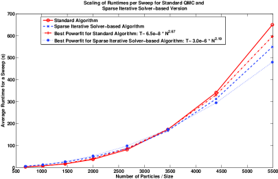
Fig. 10: The scaling of the runtime for a sweep (including all computations) for QMCPACK with its standard algorithm for determinant ratios and with the new sparse algorithm. The figure also shows the best power-law approximations for both versions.

5 Conclusions and Future Work

In this paper, we present an efficient algorithm for simulating insulators with the VMC method in the limit of large numbers of particles. Our algorithm reduces the scaling of computing the determinant ratios, the dominant computational cost for large $n$, from $O(n^{3})$ to slightly worse than $O(n^{2})$, where $n$ is the number of particles. This complements recent improvements in the scaling of constructing Slater matrices. Our main contribution is a method to compute efficiently for the Slater matrices a sequence of preconditioners that make the iterative solver converge rapidly. This involves cheap preconditioner updates, an effective reordering strategy, and a cheap method to monitor instability of the ILUTP preconditioners. Furthermore, we demonstrate experimentally that we can achieve the improved scaling without sacrificing accuracy. Our results show that preconditioned iterative solvers can reduce the cost of VMC for large(r) systems.

There are several important improvements to be explored for our proposed algorithm. First, we will implement an $O(n)$ version of the reordering algorithm. This is important for larger system sizes. We will also consider more elaborate reordering strategies like those in [16, 17]. Second, we intend to develop an incremental local reordering scheme that satisfies certain optimality properties. This should allow us to cheaply update the matrix (probably at constant cost) every Monte Carlo step or every few steps and exploit the fact that particle updates are strictly local. Potentially, the field of computational geometry might provide some insights for this effort. Third, although the ILUTP preconditioner leads to fast convergence, it is not obvious how to update the ILUTP preconditioner in its LU form. Again, the current approach with cheap intermediate, multiplicative updates by rank-one updates to the identity is effective, but it would be better to have preconditioners that can be updated continually with constant cost, local updates, and that adapt in a straightforward manner to a reordering of the matrix (at constant cost). We do not know if such preconditioners exist and whether they would yield fast convergence. In future work, we will explore forms of preconditioning that might satisfy these requirements and an underlying theory of preconditioners for Slater matrices. The latter would also include analyzing the matrix properties of Slater matrices. Fourth, an interesting experiment (also suggested by the referees) is to check whether replacing the (sparse) iterative solver by a sparse direct solver might be advantageous for certain problem sizes. We expect that for small problems the standard algorithm is fastest and for large(r) problems sparse iterative solvers are fastest. However, there might be a range of physically relevant problem sizes for which sparse direct solvers are the best. Fifth, we will extend our algorithm to other types of orbitals. One specific goal will be to adapt our algorithm to achieve quadratic scaling when the single particle orbitals are delocalized. Note that the optimization of orbitals [1, 15, 35] discussed in the Introduction leads to decaying orbitals for many systems. Finally, we will test our algorithm for realistic materials and much larger system sizes.

References

- [1] D. Alfé. Order(N) methods in QMC. 2007 Summer School on Computational Materials Science, http://www.mcc.uiuc.edu/summerschool/2007/qmc/.
- [2] D. Alfé and M. J. Gillan. An efficient localized basis set for Quantum Monte Carlo calculations on condensed matter. Physical Review B (Rapids), 70:161101 (1–4), 2004.
- [3] D. Alfé and M. J. Gillan. Linear-scaling Quantum Monte Carlo with non-orthogonal localized orbitals. Journal of Physics: Condensed Matter, 16:L305–L311, 2004.
- [4] M. P. Allen and D. J. Tildesley. Computer Simulation of Liquids. Oxford University Press, 1987.
- [5] Z. Bai, W. Chen, R. Scalettar, and I. Yamazaki. Numerical methods for Quantum Monte Carlo simulations of the Hubbard model. In T. Y. Hou, C. Liu, and J.-G. Liu, editors, Multi-Scale Phenomena in Complex Fluids, ISBN-9787040173581. Higher Education Press, China, February 2009. An early version appeared as Technical Report CSE-2007-36, Department of Computer Science, UC Davis, Dec.4, 2007 and revised on Feb.25, 2008.
- [6] M. Benzi. Preconditioning techniques for large linear systems: A survey. Journal of Computational Physics, 182(2):418 – 477, 2002.
- [7] M. Benzi, D. B. Szyld, and A. van Duin. Orderings for incomplete factorization preconditioning of nonsymmetric problems. SIAM Journal on Scientific Computing, 20(5):1652–1670, 1999.
- [8] L. Bergamaschi, R. Bru, A. Martinez, and M. Putti. Quasi-Newton preconditioners for the inexact Newton method. Electronic Transaction on Numerical Analysis, 23:76–87, 2006. http://etna.mcs.kent.edu/vol.23.2006/pp76-87.dir/pp76-87.pdf.
- [9] J. P. Boyd and K. W. Gildersleeve. Numerical experiments on the condition number of the interpolation matrices for radial basis functions. Applied Numerical Mathematics, 61:443–459, 2011.
- [10] D. Calvetti and E. Somersalo. Introduction to Bayesian Scientific Computing: Ten Lectures on Subjective Computing, volume 2 of Surveys and Tutorials in the Applied Mathematical Sciences. Springer, 2007.
- [11] D. M. Ceperley. DataSpork analysis toolkit. Materials Computation Center at the University of Illinois at Urbana-Champaign, http://www.mcc.uiuc.edu/dataspork/.
- [12] D. M. Ceperley, G. V. Chester, and M. H. Kalos. Monte Carlo simulation of a many-fermion system. Phys. Rev. B, 3081(16):3081 –3099, 1977.
- [13] M. P. Chernesky. On preconditioned Krylov subspace methods for discrete convection-diffusion problems. Numerical Methods for Partial Differential Equations, 13(4):321–330, 1997.
- [14] E. Chow and Y. Saad. Experimental study of ILU preconditioners for indefinite matrices. Journal of Computational and Applied Mathematics, 86(2):387 – 414, 1997.
- [15] N. Drummond and P. L. Rios. Worksheet 1: Using localized orbitals in QMC calculations. 2007 Summer School on Computational Materials Science, http://www.mcc.uiuc.edu/summerschool/2007/qmc/.
- [16] I. S. Duff and J. Koster. The design and use of algorithms for permuting large entries to the diagonal of sparse matrices. SIAM Journal on Matrix Analysis and Applications, 20(4):889–901, 1999.
- [17] I. S. Duff and J. Koster. On algorithms for permuting large entries to the diagonal of a sparse matrix. SIAM Journal on Matrix Analysis and Applications, 22(4):973–996, 2001.
- [18] J. M. Edmunds. Input and output scaling and reordering for diagonal dominance and block diagonal dominance. IEE Proceedings - Control Theory and Applications, 145(6):523–530, 1998.
- [19] W. M. C. Foulkes, L. Mitas, R. J. Needs, and G. Rajagopal. Quantum Monte Carlo simulations of solids. Rev. Mod. Phys., 73(1):33–83, 2001.
- [20] D. Frenkel and B. Smit. Understanding Molecular Simulation, Second Edition: From Algorithms to Applications, volume 1 of Computational Science Series. Academic Press, 2002.
- [21] G. H. Golub and C. F. Van Loan. Matrix Computations. The Johns Hopkins University Press, 1996.
- [22] A. Greenbaum. Iterative Methods for Solving Linear Systems. SIAM, 1997.
- [23] B. Hammond, W. A. Lester, and P. J. Reynolds. Monte Carlo Methods in Ab Initio Quantum Chemistry. World Scientific, Singapore, 1994.
- [24] J. Kim et al. QMCPACK. Materials Computation Center at the University of Illinois at Urbana-Champaign, http://cms.mcc.uiuc.edu/qmcpack/.
- [25] C. T. Kelley. Solving Nonlinear Equations with Newton’s Method. Society for Industrial and Applied Mathematics, 2003.
- [26] W. McMillan. Ground state of liquid helium4. Physical Review, 138(2A):A442 – A451, April 1965.
- [27] L. Mitas and J. C. Grossman. Quantum Monte Carlo study of Si and C molecular systems. in Recent Advances in Quantum Monte Carlo Methods, W. A. Lester (Ed.), pages 133–162, 1997.
- [28] P. K. V. V. Nukala and P. R. C. Kent. A fast and efficient algorithm for Slater determinant updates in Quantum Monte Carlo simulations. J. Chem. Phys., 130(204105), 2009.
- [29] Y. Saad. ILUT: a dual threshold incomplete ILU factorization. Numer. Linear Algebra Appl., 1:387–402, 1994.
- [30] Y. Saad. Iterative Methods for Sparse Linear Systems. Society for Industrial and Applied Mathematics, 3600 Market Street, Philadelphia, PA 19104-2688, USA, 2nd edition, 2003.
- [31] Y. Saad and M. H. Schultz. GMRES: A generalized minimal residual algorithm for solving nonsymmetric linear systems. SIAM Journal on Scientific and Statistical Computing, 7(3):856–869, 1986.
- [32] R. T. Scalettar, K. J. Runge, J. Correa, P. Lee, V. Oklobdzija, and J. L. Vujic. Simulations of interacting many body systems using p4. International Journal of High Speed Computing, 7(3):327–349, 1995.
- [33] J. Thijssen. Computational Physics. Cambridge University Press, 1999.
- [34] H. A. van de Vorst. Iterative Krylov Methods for Large Linear Systems. Cambridge Monographs on Applied and Computational Mathematics. Cambridge University Press, 2003.
- [35] A. J. Williamson, R. Q. Hood, and J. C. Grossman. Linear-scaling Quantum Monte Carlo calculations. Phys. Rev. Lett., 87(24):246406, 2001.