Turbulent front speed in the Fisher equation: dependence on Damköhler number

Abstract

Direct numerical simulations and mean-field theory are used to model reactive front propagation in a turbulent medium. In the mean-field approach, memory effects of turbulent diffusion are taken into account to estimate the front speed in cases when the Damköhler number is large. This effect is found to saturate the front speed to values comparable with the speed of the turbulent motions. By comparing with direct numerical simulations, it is found that the effective correlation time is much shorter than for non-reacting flows. The nonlinearity of the reaction term is found to make the front speed slightly faster.

I Introduction

It is well known that the propagation speed of a flame front is greatly enhanced if a mixture of fuel and oxygen is in a turbulent state. This topic of turbulent premixed combustion was pioneered by Damköhler D40 some 70 years ago and is reviewed extensively in recent literature Pet99 ; BPBD05 ; Dri08 . In spite of its importance, the question of burning velocities in a turbulent medium continues to be of major importance even today Kido02 ; VL06 ; Kitagawa08 .

Much of the current work is based on the original Damköhler paradigm for premixed combustion. He distinguishes two regimes, namely those of large-scale and small-scale turbulence. For the purpose of the present paper it is useful to base this distinction on a comparison of the mean turbulent flame width with the scale of the energy-carrying eddies Pet99 . In the small-scale turbulence regime, also referred to as the distributed reaction zone regime, the turbulent flame speed is computed using a formula where the microscopic diffusivity is replaced by the sum of microscopic and turbulent diffusivities. This is possible because there is good scale separation. This implies that the turbulent front thickness (i.e. the thickness of the flame brush) is much broader than the scale of the turbulent eddies. This regime is characterized by small Damköhler numbers. In the opposite case of large Damköhler numbers, the turbulent front thickness is smaller than the scale of the turbulent eddies and can therefore no longer be described by turbulent diffusion. This regime is characterized as that of large-scale turbulence. In this case the turbulent front speed reaches its maximal value that is given by the rms velocity of the turbulence in the direction of front propagation.

The regime of large-scale turbulence is subdivided further into regimes of corrugated and wrinkled flamelets, depending essentially on the ratio of Reynolds number to Damköhler number, which is also related to the Karlovitz number. When the Reynolds number is small compared with the Damköhler number (small Karlovitz number), the flame front is merely wrinkled, but for large Reynolds numbers (large Karlovitz number) it becomes corrugated and can consist of isolated flamelets detached from other parts of the front. In the present paper we will mainly be concerned with the flame speed rather than the question of whether the flame front is wrinkled or corrugated.

In turbulent combustion, the averaged flame speed, $s_{\rm T}$, is usually normalized by the corresponding laminar flame speed, $s_{\rm L}$, and one is interested in the dependence on the normalized turbulent velocity, ${v^{\prime}}$. For the regime of large-scale turbulence, the speed-up ratio of turbulent to laminar flame speed is given by the geometric increase of the wrinkled surface area of the flame front. Damköhler assumed that the increase in surface area is proportional to the ratio of the turbulent velocity of the eddies to the laminar flame speed. This leads to the expectation that the dependence of $s_{\rm T}$ on ${v^{\prime}}$ is given by Pet99

$$s_{\rm T}/s_{\rm L}=1+{v^{\prime}}/s_{\rm L}.$$ (1)

This equations captures the expected limiting cases that $s_{\rm T}$ should not become larger than ${v^{\prime}}$ and that $s_{\rm T}=s_{\rm L}$ in the absence of turbulence, i.e., for ${v^{\prime}}=0$. However, unsatisfactory agreement with measurements motivated the search for other dependencies. For example, Pocheau Poc92 derives the more general formula

$$s_{\rm T}/s_{\rm L}=\left[1+\left({v^{\prime}}/s_{\rm L}\right)^{n}\right]^{1/n},$$ (2)

where $n$ is a parameter. This formula obeys the aforementioned limiting case for any value of $n$. Pocheau Poc92 contrasts the formula with another one proposed by Yakhot Yak88 ,

$$s_{\rm T}/s_{\rm L}=\exp\left[\left({v^{\prime}}/s_{\rm T}\right)^{2}\right],$$ (3)

where $s_{\rm T}<{v^{\prime}}$ for ${v^{\prime}}\to\infty$. Yet another fit formula is given by

$$s_{\rm T}/s_{\rm L}=1+C_{\rm W}\left({v^{\prime}}/s_{\rm L}\right)^{m}$$ (4)

with fit parameters $C_{\rm W}$ and $m=0.7$ Wil85 . Both (3) and (4) have a front speed less than $v^{\prime}$ for ${v^{\prime}}\to\infty$, provided $m<1$ in Eq. (4). As can be seen from Fig. 1, the different proposals for the front speed are quite similar, making it difficult to use measurements to distinguish between them. Furthermore, realistic descriptions of flame properties are hampered by the fact that feedback on the flow by the actual combustion process depends to the specific case and is not easy to model. The feedback on the flow is therefore usually ignored. It might therefore be useful to return to a simple model of front propagation that can be treated in more detail and to address the unsettled question regarding the different proposals in Eqs (1)–(4) for the dependence of $s_{\rm T}$ on ${v^{\prime}}$. Following Kerstein Ker02 , we consider here the Fisher equation, which is also known as the Kolmogorov–Petrovskii–Piskunov (KPP) equation KPP37 . An important difference to earlier work is the fact that we solve this equation in the three-dimensional case in the presence of a turbulent velocity field.

The Fisher or KPP equation is a simple scalar equation that possesses propagating front solutions. This equation is familiar in biomathematics Mur93 as a simple model for the spreading of diseases. It has also been amended by an advection term to describe the interaction with a turbulent velocity field in one BN09 and multiple PBNT10 dimensions, the effects of cellular flows CTVV03 , and the scaling of the front thickness BVV08 . Furthermore the equation has also been modified to account for different interacting species, that can be used to model the spreading of auto-catalytically polymerizing left and right handed nucleotides BM04 . Given that $C$ is a passive (albeit reacting) scalar, the Fisher equation does ignore any feedback on the flow and is therefore well suited to help clarifying questions regarding the relation between $s_{\rm T}$ and ${v^{\prime}}$.

Figure 1: Comparison of different expressions for the normalized front speed, $s_{\rm T}/s_{\rm L}$, as a function of the turbulent velocity, ${v^{\prime}}/s_{\rm L}$. The labels $n=1$ and $n=2$ refer to Eqs. (1) and (2), while Y88 and W85 refer to Eqs. (3) and (4).

In the present paper we consider both direct numerical simulations (DNS) of this equation in three dimensions as well as its averaged form where the effects of turbulence are being parameterized by a non-Fickian diffusion equation. Such an equation allows for the ballistic spreading of a passive scalar concentration on short time scales, which is expected to be important when the front propagates at a speed comparable to that of the turbulence itself.

II The Fisher equation

A simple model of front propagation is the Fisher equation which, in the simplest case, is a one-dimensional partial differential equation Mur93 ; KPP37 ; Fis37 ; Kal84 ,

$$\frac{\partial C}{\partial t}={C\over\tau_{\rm c}}\left(1-{C\over C_{0}}\right)+D\frac{\partial^{2}C}{\partial x^{2}},$$ (5)

for the concentration $C$. Here, $\tau_{\rm c}$ is the chemical reaction time, $D$ is the diffusivity, and $C_{0}$ is some saturation value above which further growth is quenched. Equation (5) corresponds to an autocatalytic reaction were a reactant ${\cal R}$ yields a product ${\cal P}$ at a rate $k$ that is itself proportional to the concentration of the products, $[{\cal P}]$, i.e.

$${\cal R}\stackrel{{\scriptstyle k~{}}}{{\longrightarrow}}{\cal P}\quad\mbox{with}\quad k=[{\cal P}]/\tau_{\rm c}C_{0}.$$ (6)

This can then also be written as ${\cal P}+{\cal R}\to 2{\cal P}$. Saturation of the product concentration, $C=[{\cal P}]$, results from the fact that the total mass is conserved, i.e. $[{\cal R}]+[{\cal P}]=C_{0}=\rm const$. The evolution equation for the concentration $C=[{\cal P}]$ is then given by Eq. (5).

This equation has two solutions, an unstable solution, $C=0$, and a stable one, $C=C_{0}$. The diffusion term seeds the neighboring regions that are in an unstable state, which promotes the rapid transition from $C=0$ to $C=C_{0}$. This leads to the propagation of the transition front in the direction down the gradient of $C$ with a front speed Mur93

$$s_{\rm L}=2\sqrt{D/\tau_{\rm c}},$$ (7)

where the subscript L refers to the laminar front speed.

In many cases of practical interest the diffusion coefficient $D$ is rather small and is hardly relevant when there is rapid advection through fluid motions. In that case the governing equations become advection–reaction–diffusion equations. This can be written as

$$\frac{\partial C}{\partial t}+\bm{\nabla}\cdot(\bm{U}C)={C\over\tau_{\rm c}}\left(1-{C\over C_{0}}\right)+D\nabla^{2}C,$$ (8)

where $\bm{U}$ is the flow speed. If the flow is turbulent and has zero mean, there can be circumstances where the average concentration $\overline{C}$ can be described by an equation similar to Eq. (5), but with $C$ being replaced by the mean value $\overline{C}$, and $D$ being replaced by some turbulent diffusivity $D_{\rm t}$, i.e.

$$\frac{\partial\overline{C}}{\partial t}={\overline{C}\over\tau_{\rm c}}\left(1-{\overline{C}\over C_{0}}\right)+D_{\rm T}\frac{\partial^{2}\overline{C}}{\partial x^{2}},$$ (9)

where $D_{\rm T}=D+D_{\rm t}$ is the total (i.e. the sum of microscopic and turbulent) diffusivity. We have here assumed that the mean concentration shows a systematic variation in the $x$ direction and have thus assumed averaging over the $y$ and $z$ directions, so $\overline{C}(x,t)$ can be described by a one-dimensional evolution equation.

Given the similarity between Eqs. (5) and (9), one would expect that in the turbulent case with appropriate initial conditions the effective turbulent propagation speed $s_{\rm T}$ of the front can still be described by an expression similar to Eq. (7), but with $D$ being replaced by $D_{\rm T}$, i.e. $s_{\rm T}=2\sqrt{D_{\rm T}/\tau_{\rm c}}$. A useful estimate for the turbulent diffusivity is $D_{\rm t}=u_{\rm rms}/3k_{\rm t}$, where $k_{\rm t}$ is the wavenumber of the energy-carrying eddies and $u_{\rm rms}$ is the rms velocity of the turbulence BSV09 . Thus, for $D_{\rm t}\gg D$, the effective value of $s_{\rm T}$ is expected to be $2(u_{\rm rms}/3\tau_{\rm c}k_{\rm t})^{1/2}$. On the other hand, one cannot expect the front speed to increase indefinitely with decreasing $\tau_{\rm c}$. Indeed, one would not expect $s_{\rm T}$ to exceed the rms velocity of the turbulence in the direction of front propagation. Following common practice, we denote it by ${v^{\prime}}$. Under the assumption of isotropy, ${v^{\prime}}$ is related to the three-dimensional rms velocity by ${v^{\prime}}=u_{\rm rms}/\sqrt{3}$.

An important nondimensional measure of $\tau_{\rm c}$ is the Damköhler number, which is the ratio of the turnover time, $(u_{\rm rms}k_{\rm t})^{-1}$, to $\tau_{\rm c}$. This number is here defined as

$$\mathrm{Da}=(\tau_{\rm c}u_{\rm rms}k_{\rm t})^{-1}.$$ (10)

Note that our definition of Da is based on the wavenumber $k_{\rm t}$ rather than the scale $2\pi/k_{\rm t}$, which would have reduced the numerical value of Da by a factor of $2\pi$. For small values of $\mathrm{Da}$ we expect $s_{\rm T}\approx 2{v^{\prime}}\,\mathrm{Da}^{1/2}$, while for large values one expects $s_{\rm T}\approx{v^{\prime}}$ Poc92 . Thus, a more general formula is expected to be

$$s_{\rm T}^{2}={v^{\prime}}^{2}f(\mathrm{Da}),$$ (11)

where $f(\mathrm{Da})$ increases linearly with $\mathrm{Da}$ for $\mathrm{Da}\ll 1$ and $f(\mathrm{Da})\approx 1$ for $\mathrm{Da}\gg 1$. This saturation behavior can also be interpreted as a reduction of the effective value of $\tau_{\rm c}$ EKR98 . An important goal of this paper is to determine the form of the function $f(\mathrm{Da})$.

III Non-Fickian diffusion

The Fickian diffusion approximation made in Eq. (9) for the mean concentration $\overline{C}$ becomes invalid if $\overline{C}$ varies rapidly in time, and in principle also in space. This is indeed expected to be the case when $\mathrm{Da}\gg 1$. For rapid time variations, Eq. (9) attains then an extra time derivative and takes the form BKM04

$$\tau\frac{\partial^{2}\overline{C}}{\partial t^{2}}+\frac{\partial\overline{C}}{\partial t}={\overline{C}\over\tau_{\rm c}}\left(1-{\overline{C}\over C_{0}}\right)+D_{\rm T}\frac{\partial^{2}\overline{C}}{\partial x^{2}},$$ (12)

which is a damped wave equation with relaxation time $\tau$ and an additional reaction term. The presence of the nonlinearity in the reaction term leads to an additional contribution in the $\overline{C}$ equation which has here been ignored (see Appendix A for a more consistent treatment).

Without the reaction term, Eq. (12) is also known as the telegraph equation. This equation emerges naturally when computing turbulent transport coefficients using the $\tau$ approximation BF03 . Evidence for the existence of the wave term has been found from isotropic forced turbulence simulations BKM04 . A non-dimensional measure of $\tau$ is given by the Strouhal number,

$$\mathrm{St}=\tau u_{\rm rms}k_{\rm t}=\tau u_{\rm rms}^{2}/3D_{\rm t},$$ (13)

where the first equality is useful for turbulence simulations where $\tau u_{\rm rms}k_{\rm t}$ is readily evaluated, while the second equality is useful for the mean-field model, where $k_{\rm t}$ does not appear explicitly and $D_{\rm t}$ and $u_{\rm rms}$ are given.

Using DNS of forced turbulence with a passive scalar, the value of St has been determined to be around 3 by relating triple corrections to quadratic ones BKM04 . Although we consider the value of St as being fairly well constrained, we do consider below a range of different values.

The purpose of this section is to study solutions of Eq. (12) that can then be compared with DNS of the Fisher equation coupled with the Navier-Stokes equations for obtaining a turbulent velocity that enters Eq. (8). We consider first the case where $D$ is negligible and solve Eq. (12) for different values of Da in a one-dimensional domain that was chosen long enough so that the front speed can be determined accurately enough. We use a numerical scheme that is second order in space and third order in time BD02 . In some cases a resolution of $2^{15}\approx 3\times 10^{4}$ mesh points was necessary.

Figure 2: Dependence of the front speed of solutions of Eq. (12) on Da for different values of St and $\mathrm{Pe}=\infty$. The lines represent fits given by Eq. (15).

We study first the dependence of the front speed on Da for a range of different values of St and $D\ll D_{\rm t}$. Here, $s_{\rm T}$ is determined by differentiating the concentration integrated over the whole domain,

$$s_{\rm T}(t)={\mathrm{d}\over\mathrm{d}t}\int{\overline{C}\over C_{0}}\,\mathrm{d}z,$$ (14)

and approximating the asymptotic front speed with the value at the time when the front has reached the other end of the domain. This quantity is also known as the reaction speed. This is indicated by $\overline{C}$ reaching a small fraction (e.g. $10^{-6}$) of $C_{0}$. The result is shown in Fig. 2. For small values of Da, the front speed is independent of the value of St and we reproduce the anticipated result, i.e. $f(\mathrm{Da})=4\,\mathrm{Da}$. For larger values of Da the front speed reaches eventually a constant value. However, the limiting value depends on St. Our results are well reproduced by the fit formula

$${s_{\rm T}^{2}\over{v^{\prime}}^{2}}\equiv f(\mathrm{Da},\,\mathrm{St})\approx{4\,\mathrm{Da}\over 1+3\,\mathrm{St}\,\mathrm{Da}}.$$ (15)

This formula obeys the anticipated limiting behaviors for small and large values of Da, provided $\mathrm{St}\approx 4/3$. The numerically determined data agree quite well with Eq. (15). However, in some cases the numerical data are somewhat uncertain and depend also slightly on resolution and domain size.

In the DNS presented below, where the numerical resolution is still limited, the value of $D$ is often not negligible. Its value is characterized by the Peclet number,

$$\mathrm{Pe}=u_{\rm rms}/Dk_{\rm t}\approx 3D_{\rm t}/D.$$ (16)

For small values of Da, the expression for the front speed should be $s_{\rm T}=2\sqrt{(D_{\rm t}+D)/\tau_{\rm c}}$, which can then be written as

$$s_{\rm T}/{v^{\prime}}=2\sqrt{\left(1+3\mathrm{Pe}^{-1}\right)\mathrm{Da}}\quad\mbox{(for $\mathrm{Da}\ll 1$)}.$$ (17)

For larger values of $\mathrm{Da}$ we solve Eq. (12) numerically. A good fit formula for $f$ is given by

$$f(\mathrm{Da},\,\mathrm{St},\,\mathrm{Pe})\approx 4\mathrm{Da}\left({3\over\mathrm{Pe}}+{1\over 1+3\mathrm{St}\,\mathrm{Da}}\right).$$ (18)

In Fig. 3 we compare the fit formula with the numerically obtained front speeds for different values of Pe, keeping $\mathrm{St}=3$. The agreement is again quite good.

Figure 3: Dependence of the front speed of solutions of Eq. (12) on Da for different values of Pe and $\mathrm{St}=3$. The lines represent fits given by Eq. (18).

In turbulent combustion it is customary to plot the normalized front speed, $s_{\rm T}/s_{\rm L}$, as a function of the normalized turbulent velocity, ${v^{\prime}}/s_{\rm L}$. Using our definitions of $\mathrm{Da}$ and $\mathrm{Pe}$ in Eqs. (10) and (16), respectively, we have ${v^{\prime}}/s_{\rm L}=({\mathrm{Pe}/12\,\mathrm{Da}})^{1/2}$ and find

$${s_{\rm T}\over s_{\rm L}}=\left[1+{1\over 3\mathrm{St}/4+\epsilon{v^{\prime}}/s_{\rm L}}\left({{v^{\prime}}\over s_{\rm L}}\right)^{2}\right]^{1/2},$$ (19)

where we have defined $\epsilon=k_{\rm t}\ell_{\rm F}$ with $\ell_{\rm F}=(\tau_{\rm c}D/12)^{1/2}$ being a measure for the laminar flame thickness. Note that $\epsilon$ can also be expressed in terms of Da and Pe via

$$\epsilon=(12\mathrm{Da}\,\mathrm{Pe})^{-1/2}.$$ (20)

A more familiar quantity is the ratio $\ell/\ell_{\rm F}=\epsilon^{-1}$, where $\ell=k_{\rm t}^{-1}$ is the typical eddy scale. Even if we can assume the value of St to be given, $\epsilon$ is not a fixed quantity. It is therefore clear that there cannot be a unique relationship between $s_{\rm T}/s_{\rm L}$ and ${v^{\prime}}/s_{\rm L}$. Instead, there must be a family of solutions depending on the value of $\epsilon$; see Fig. 4.

Figure 4: Dependence of $s_{\rm T}/s_{\rm L}$ and ${v^{\prime}}/s_{\rm L}$ for $\epsilon=0$ (solid line), 0.3 (dotted), 1 (dashed), and 3 (dash-dotted). Note that there is no unique relationship between $s_{\rm T}/s_{\rm L}$ and ${v^{\prime}}/s_{\rm L}$.

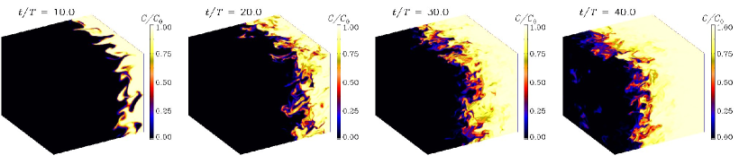
Figure 5: Visualization of the concentration $C$ on the periphery of the box at different times for Run A1. Here, $T=(u_{\rm rms}k_{\rm t})^{-1}$ is the turnover time.

IV DNS of the Fisher equation

We now consider DNS of Eq. (8) where $\bm{U}$ is obtained by solving the Navier-Stokes equation for an isothermal gas with a forcing term that is $\delta$ correlated in time. The forcing function consists of plane waves whose wave vector is random and its length is within a narrow window around some mean forcing wavenumber $k_{\rm t}$. Since the gas is compressible and the density $\rho$ is not constant, Eq. (8) now takes the form

$$\frac{\partial C}{\partial t}+\bm{U}\cdot\bm{\nabla}C={C\over\tau_{\rm c}}\left(1-{C\over C_{0}}\right)+\bm{\nabla}\cdot\left(\rho D\bm{\nabla}{C\over\rho}\right),$$ (21)

which we solve together with the momentum and continuity equations,

$${\partial\bm{U}\over\partial t}=-\bm{U}\cdot\bm{\nabla}\bm{U}-c_{\rm s}^{2}\bm{\nabla}\ln\rho+\bm{f}+\bm{F}_{\rm force},$$ (22)

$${\partial\rho\over\partial t}=-\bm{\nabla}\cdot\rho\bm{U},$$ (23)

where $\bm{F}_{\rm force}=\nu(\nabla^{2}\bm{U}+{\textstyle{\frac{1}{3}}}\bm{\nabla}\bm{\nabla}\cdot\bm{U}+2\bm{\mathsf{S}}\bm{\nabla}\ln\rho)$ is the viscous force, $\bm{\mathsf{S}}={\textstyle{\frac{1}{2}}}\left[\bm{\nabla}\bm{U}+(\bm{\nabla}\bm{U})^{\rm T}\right]-{\textstyle{\frac{1}{3}}}\bm{\mathsf{I}}\bm{\nabla}\cdot\bm{U}$ is the traceless rate of strain tensor, $\bm{\mathsf{I}}$ is the unit matrix, $\nu$ is the molecular diffusivity, and $c_{\rm s}=\rm const$ is the isothermal sound speed. The forcing function $\bm{f}$ is of the form

$$\bm{f}(\bm{x},t)=\mathrm{Re}\{N\bm{f}_{\bm{k}(t)}\exp[\mathrm{i}\bm{k}(t)\cdot\bm{x}+\mathrm{i}\phi(t)]\},$$ (24)

where $\bm{x}$ is the position vector. The wave vector $\bm{k}(t)$ and the random phase $-\pi<\phi(t)\leq\pi$ change at every time step. For the time-integrated forcing function to be independent of the length of the time step $\delta t$, the normalization factor $N$ has to be proportional to $\delta t^{-1/2}$. On dimensional grounds it is chosen to be $N=f_{0}c_{\rm s}(k_{\rm t}c_{\rm s}/\delta t)^{1/2}$, where $f_{0}$ is a nondimensional forcing amplitude. The value of the coefficient $f_{0}$ is chosen such that the maximum Mach number stays below about 0.5. Here we choose $f_{0}=0.02$. We force the system with nonhelical transversal waves,

$$\bm{f}_{\bm{k}}=\left(\bm{k}\times\bm{e}\right)/\sqrt{\bm{k}^{2}-(\bm{k}\cdot\bm{e})^{2}},$$ (25)

where $\bm{e}$ is an arbitrary unit vector not aligned with $\bm{k}$; note that $|\bm{f}_{\bm{k}}|^{2}=1$.

In the $x$ direction we use periodic boundary conditions for $\bm{U}$ and $\rho$ and $\partial C/\partial x=0$ for $C$, while we use periodic boundary conditions in the $y$ and $z$ directions. The simulations were performed with the Pencil Code PencilCode , which uses sixth-order explicit finite differences in space and a third-order accurate time stepping method BD02 .

For the calculations we use units where $k_{1}=c_{\rm s}=\rho_{0}=1$. However, most of the results are presented in an explicitly non-dimensional form by normalizing with respect to relevant quantities such as the rms velocity of the turbulence or the turnover time. Our simulations are characterized by several non-dimensional parameters. In addition to the values of Da and Pe, defined in Eqs. (5) and (16), respectively, there is the Schmidt number, $\mathrm{Sc}=\nu/D$. In those cases where the Damköhler number was large, we had to increase the value of $D$ in order to resolve the flame front. This was done by decreasing $\mathrm{Sc}$ to values below unity. The degree of scale separation is given by the ratio $k_{\rm t}/k_{1}$.

Table 1: Summary of the runs discussed in this paper.

Run	$A$	Re	Pe	Da	Ka	$k_{\rm t}/k_{1}$	$s_{\rm T}/{v^{\prime}}$	$s_{\rm T}/s_{\rm L}$	${v^{\prime}}/s_{\rm L}$	$\ell/\ell_{\rm F}$
A1	$1$	$117$	$117$	$0.2$	$14.6$	$5.0$	$0.97$	$7.50$	$7.75$	$15.0$
A2	$1$	$115$	$115$	$0.5$	$4.8$	$5.1$	$1.60$	$7.03$	$4.38$	$26.3$
A3	$1$	$122$	$49$	$1.6$	$3.6$	$5.1$	$2.33$	$3.77$	$1.61$	$30.4$
A4	$1$	$121$	$12$	$4.8$	$4.8$	$5.1$	$3.55$	$1.63$	$0.46$	$26.3$
A5	$1$	$120$	$4$	$15.9$	$3.6$	$5.1$	$7.29$	$1.16$	$0.16$	$30.3$
B1	$4$	$38$	$513$	$1.6$	$3.6$	$1.6$	$1.88$	$9.76$	$5.19$	$98.9$
B2	$2$	$41$	$164$	$4.9$	$3.6$	$1.6$	$2.21$	$3.69$	$1.67$	$98.8$
B3	$2$	$165$	$165$	$4.9$	$3.6$	$1.6$	$2.52$	$4.22$	$1.67$	$98.9$
B4	$2$	$41$	$16$	$4.9$	$36.4$	$1.6$	$2.80$	$1.47$	$0.53$	$31.3$
B5	$2$	$40$	$16$	$50.3$	$3.6$	$1.6$	$7.25$	$1.19$	$0.16$	$98.9$

V Results

In the following we present results for uniform aspect ratio, $A=L_{x}/L_{y}=1$ with $k_{\rm t}/k_{1}=5$ (series A), and $A=2$ or 4 with $k_{\rm t}/k_{1}=1.6$ (series B). Our runs of series A and B are summarized in Table 1. The resolution in the $y$ and $z$ directions is always $256^{2}$ meshpoints, but it is larger in the $x$ direction in runs where the aspect ratio $A$ is larger than unity. In Fig. 5 we show the concentration $C$ on the periphery of the computational domain at different times for $\tau_{\rm c}=3/c_{\rm s}k_{1}$, which corresponds to $\mathrm{Da}=0.5$; see Table 1. One sees clearly how the front spreads and propagates in the negative $x$ direction. The front speed is determined in the same way as for the mean-field model, i.e. using Eq. (14), except that $\overline{C}$ is computed from the actual $C$. This can also be formulated as a volume integral,

$$s_{\rm T}(t)={1\over L_{x}L_{y}}{\mathrm{d}\over\mathrm{d}t}\int{C\over C_{0}}\,\mathrm{d}V.$$ (26)

In Fig. 6 we show examples of the evolution of the mean concentration and the instantaneous front speed as functions of time for series A. The resulting ratios $s_{\rm T}/{v^{\prime}}$, $s_{\rm T}/s_{\rm L}$, ${v^{\prime}}/s_{\rm L}$, and $\ell/\ell_{\rm F}$ are summarized in Table 1 for series A and B.

Figure 6: Mean concentration and the instantaneous front speed as functions of time.

In most of the cases considered in this paper, the value of $\mathrm{Pe}$ is not in the asymptotic regime. It might therefore be sensible to compare the relative front speed, $s_{\rm T}/{v^{\prime}}$ against the function $f(\mathrm{Da},\,\mathrm{St},\,\mathrm{Pe})$. This is done in Fig. 7, where we show the non-dimensional front speed, $s_{\rm T}/{v^{\prime}}$, versus $f(\mathrm{Da},\,\mathrm{St},\,\mathrm{Pe})$, for three values of St using values of Da and Pe, as evaluated from Eqs. (10) and (16). Surprisingly, the best fit is obtained for rather small values of St of 0.03. This suggests that, for the present applications, the relevant value of $\tau$ is much smaller than in the case of a non-reacting passive scalar.

Figure 7: Relative front speed as a function of $f$ for three values of St. The squares indicate runs where the fluid is at rest and the front is moving through the domain while the asterisk denote runs with an inlet velocity chosen such that the front is approximately stationary within the domain. The solid line gives the theoretically expected result, $s_{\rm T}/{v^{\prime}}=f(\mathrm{Da},\,\mathrm{St},\,\mathrm{Pe})^{1/2}$. Note that the best agreement with the theoretical values is achieved for St=0.03.

Figure 8: Relative turbulent front speed versus Da. The squares indicate runs where the fluid is at rest and the front is moving through the domain while the asterisk denote runs with an inlet velocity chosen such that the front is approximately stationary within the domain. For the latter, big asterisks denote cases where $\mathrm{Pe}>10$. The lines give the theoretical expectations for $\mathrm{St}=0.03$ and Pe=1 (solid line), 10 (dotted), and 100 (dashed line).

Next, we plot $s_{\rm T}/{v^{\prime}}$ versus Da for different values of Pe; see Fig. 8 using the previously inferred value St=0.03. The data points from the DNS tend to lie between the curves for $\mathrm{Pe}=1$ and 10, even though most of the actual values of Pe are beyond Pe=10. This too suggests some inconsistency between the DNS and the mean-field description in terms of the telegraph equation. Finally we plot the DNS results in a state diagram of $s_{\rm T}/s_{\rm L}$ versus ${v^{\prime}}/s_{\rm L}$ using St=0.03; see Fig. 9. The data lie between the theoretical curves for $\ell/\ell_{\rm F}=10$ and 100, which is roughly in agreement with the values given in Table 1.

Figure 9: Turbulent front speed versus turbulence intensity for $\epsilon=0.1$ (solid line), 1 (dotted), and 10 (dashed) using $\mathrm{St}=0.03$. The squares indicate runs where the fluid is at rest and the front is moving through the domain while the asterisk denote runs with an inlet velocity chosen such that the front is approximately stationary within the domain. For the latter, big asterisks denote cases where $\mathrm{Pe}>10$. The lines give the theoretical expectations.

VI Conclusions

In the present work, the Fisher equation has served as a simple model equation for front propagation in a turbulent flow. The model has similarities with turbulent combustion, but is much simpler. Nevertheless, it is clear that even this simple model harbors surprises that one might have overlooked under more complex conditions. Using three-dimensional simulations we have been able to compare with the associated mean-field model. For small Damköhler numbers, the effective front speed can be approximated by replacing the diffusivity by a turbulent value. However, for Damköhler numbers larger than unity, this simple procedure fails, because it would suggest front speeds that exceed the characteristic speed of the turbulent eddies. A simple remedy is then to use a non-Fickian diffusion law for the turbulent diffusion and to retain the time derivative in the expression for the concentration flux. Earlier work did already confirm the principal validity of this approach and resulted in an estimate for the relevant relaxation time, which is characterized by the Strouhal number. The current work shows that the best fit to the simulation data can be achieved with a Strouhal number that is as small as 0.03, which is about 100 times smaller than the earlier determined value for passive scalar diffusion in forced turbulence. This difference is connected with the presence of a reaction term in the evolution equation for the passive scalar concentration.

Appendix A Mean-field effect of the reaction term

In order to assess the effect of neglecting the reaction term in the analysis presented above, we present now a simple mean-field theory for the Fisher equation using the $\tau$ equation. We start with the passive scalar equation with a reaction term as given by Eq. (8), split $C=\overline{C}+c$ and $\bm{U}=\overline{\bm{U}}+\bm{u}$ into mean and fluctuating parts, neglect the molecular diffusion term for simplicity, and define the mean concentration flux $\overline{\mbox{\boldmath${\cal F}$}}{}=\overline{\bm{u}c}$ and the mean squared concentration, $\overline{\cal H}=\overline{c^{2}}$, so the equation for the mean concentration is

$${\partial\overline{C}\over\partial t}=-\bm{\nabla}\cdot(\overline{\bm{U}}\,\overline{C}+\overline{\mbox{\boldmath${\cal F}$}}{})+{\overline{C}\over\tau_{\rm c}}\left(1-{\overline{C}\over C_{0}}\right)-{\overline{\cal H}\over\tau_{\rm c}C_{0}},$$ (27)

so the equation for the fluctuations is, to linear order in the fluctuations,

$${\partial c\over\partial t}=-\bm{\nabla}\cdot(\overline{\bm{U}}c+\bm{u}\overline{C})+{c\over\tau_{\rm c}}\left(1-{2\overline{C}\over C_{0}}\right)+...$$ (28)

where the dots denote higher order terms for which we shall adopt a general closure assumption. Next, we derive evolution equations for $\overline{\mbox{\boldmath${\cal F}$}}{}$ and $\overline{\cal H}$, ignore a mean flow for simplicity, and assume $\bm{\nabla}\cdot\bm{u}=0$, so we have

$${\partial\overline{\mbox{\boldmath${\cal F}$}}{}\over\partial t} = -\tilde{D}_{\rm t}\bm{\nabla}\overline{C}+{\overline{\mbox{\boldmath${\cal F}$}}{}\over\tau_{\rm c}}\left(1-{2\overline{C}\over C_{0}}\right)-{\overline{\mbox{\boldmath${\cal F}$}}{}\over\tau},$$ (29)

$${\partial\overline{\cal H}\over\partial t} = -2\overline{\mbox{\boldmath${\cal F}$}}{}\cdot\bm{\nabla}\overline{C}+2{\overline{\cal H}\over\tau_{\rm c}}\left(1-{2\overline{C}\over C_{0}}\right)-{\overline{\cal H}\over\tau}.$$ (30)

In Eqs. (29) and (30) we can write the last two terms as $-\overline{\mbox{\boldmath${\cal F}$}}{}/\tau_{{\cal F}}$ and $-\overline{\cal H}/\tau_{{\cal H}}$, respectively, where

$${1\over\tau_{{\cal F}}(\overline{C})} = {1\over\tau}-{1\over\tau_{\rm c}}\left(1-{2\overline{C}\over C_{0}}\right),$$ (31)

$${1\over\tau_{{\cal H}}(\overline{C})} = {1\over\tau}-{2\over\tau_{\rm c}}\left(1-{2\overline{C}\over C_{0}}\right).$$ (32)

On sufficiently long time scales we may ignore the time derivatives in Eqs. (29) and (30), so we arrive at closed expressions for $\overline{\mbox{\boldmath${\cal F}$}}{}$ and $\overline{\cal H}$, that we insert into Eq. (27), so we obtain

$${\partial\overline{C}\over\partial t}+\bm{U}_{\rm c}\cdot\bm{\nabla}\overline{C}={\overline{C}\over\tau_{\rm c}}\left(1-{\overline{C}\over C_{0}}\right)+D_{\rm T}\nabla^{2}\overline{C},$$ (33)

where $\bm{U}_{\rm c}(\overline{C})$ is a new effective advection speed and $D_{\rm T}=D+D_{\rm t}$ is again the sum of turbulent and microscopic diffusivities with

$$\bm{U}_{\rm c}(\overline{C})=2D_{\rm t}{\tau_{{\cal H}}\over\tau_{\rm c}}{\bm{\nabla}\overline{C}\over C_{0}},\quad D_{\rm t}(\overline{C})=\tau_{{\cal F}}(\overline{C})\,{v^{\prime}}^{2}.$$ (34)

One may expect that the term $\bm{U}_{\rm c}$ slows down the propagation speed of the front, because it is directed up the concentration gradient. Note that the sign of the $\bm{U}_{\rm c}$ term is opposite to that of a similar term in the so-called $G$ equation Pet99 ; Wil85 of turbulent front propagations, which is however not an equation for the flame brush, but for the detailed position of the wrinkled flame front (at $G=0$) with an advection speed that is given by $\bm{u}-s_{\rm L}\hat{\mbox{\boldmath$n$}}{}$, where $\hat{\mbox{\boldmath$n$}}{}=\bm{\nabla}G/|\bm{\nabla}G|$ is a unit vector normal to the flame front, but it enters with a minus sign and thus corresponds to an enhanced speed down the gradient of $G$. However, by solving Eq. (27) with Eqs. (29) and (30), it turns that when the $\overline{\cal H}$ term is included, it accelerates the front; see Table 2. Note also that the coefficient $D_{\rm t}$ is reduced and can even become negative in the unstable part of the front where $C=0$ (or at least $C<C_{0}/2$); see Eqs. (31) and (34). In that case our expression for turbulent diffusion becomes invalid and one has to include higher order derivatives that would guarantee stability at small length scales.

Table 2: Dependence of $s_{\rm T}/{v^{\prime}}$ without and with $\overline{\cal H}$ in a model for $\mathrm{Pe}=10$. Note the slight increase of $s_{\rm T}/{v^{\prime}}$ when $\overline{\cal H}$ compared to the case where it is neglected.

Da	$s_{\rm T}/{v^{\prime}}$(without $\overline{\cal H}$)	$s_{\rm T}/{v^{\prime}}$(with $\overline{\cal H}$)
0.10	0.25	0.25
0.30	0.44	0.47
0.50	0.59	0.65
0.61	0.66	0.73

- (1) G. Damköhler, Elektrochem. angew. Phys. Chem. 46, 601 (1940).
- (2) N. Peters, J. Fluid Mech. 384, 107 (1999).
- (3) R. W. Bilger, S. B. Pope, K. N. C. Bray and J. F. Driscoll, Proc. Combust. Inst. 30, 21 (2005).
- (4) J. F. Driscoll, Prog. Energy Comb. Sci. 34, 91 (2008).
- (5) H. Kido, M. Nakahara, K. Nakashima and J. Hashimoto, Proc. Combust. Inst. 29, 1855 (2002).
- (6) V. R. Savarianandam and C. J. Lawn, Combust. Flame. 146, 1 (2006).
- (7) T. Kitagawa, T. Nakahara, K. Maruyama, K. Kado, A. Hayakawa, and S. Kobayashi, Int. J. Hydrogen Energy 33, 5842 (2008).
- (8) A. Pocheau, Europhys. Lett. 20, 401 (1992).
- (9) V. Yakhot, Combust. Sci. Technol. 60, 191 (1988).
- (10) F. A. Williams, Combustion Theory. Addison-Wesley (1985).
- (11) A. R. Kerstein, Proc. Combust. Inst. 29, 1763 (2002).
- (12) J. D. Murray, Mathematical Biology. An introduction. Springer, New York (2002).
- (13) A. Brandenburg, A. Svedin, G. M. Vasil, Monthly Notices Roy. Astron. Soc. 395, 1599 (2009).
- (14) R. Benzi and D. R. Nelson, Physica D 238, 2003 (2009).
- (15) P. Perlekar, R. Benzi, D. R. Nelson, F. Toschi, eprint arXiv:1006.3204 (2010)
- (16) M. Cencini, A. Torcini, D. Vergni, and A. Vulpiani, Phys. Fluids 15, 679 (2003).
- (17) S. Berti, D. Vergni, and A. Vulpiani, Europhys. Lett. 83, 54003 (2008).
- (18) A. Brandenburg and T. Multamäki, Int. J. Astrobiol. 3, 209 (2004).
- (19) A. N. Kolmogorov, I. G. Petrovskii, and N. S. Piskunov, Moscow Univ. Bull. Math. 1, 1 (1937).
- (20) R. A. Fisher, Ann. Eugenics 7, 353 (1937).
- (21) P. Kaliappan, Physica D 11, 368 (1984).
- (22) The Pencil Code is a high-order finite-difference code (sixth order in space and third order in time) for solving the compressible MHD equations; http://pencil-code.googlecode.com.
- (23) E. G. Blackman and G. B. Field, Phys. Fluids 15, L73 (2003).
- (24) T. Elperin, N. Kleeorin, and I. Rogachevskii, Phys. Rev. Lett. 80, 69 (1998).
- (25) A. Brandenburg, P. Käpylä, and A. Mohammed, A., Phys. Fluids 16, 1020 (2004).
- (26) A. Brandenburg and W. Dobler, Comp. Phys. Comm. 147, 471 (2002).
- (27) G. Lodato, P. Domingo, L. Vervisch, J. Comp. Phys. 227, 5105 (2008).