Reentrance effect in macroscopic quantum tunneling
and non-adiabatic Josephson dynamics in $d$-wave junctions

Abstract

We develop a theoretical description of non-adiabatic Josephson dynamics in superconducting junctions containing low energy quasiparticles. Within this approach we investigate the effects of midgap states in junctions of unconventional d-wave superconductors. We identify a reentrance effect in the transition between thermal activation and macroscopic quantum tunneling, and connect this phenomenon to the experimental observations in Phys. Rev. Lett. 94, 087003 (2005). It is also shown that nonlinear Josephson dynamics can be defined by resonant interaction with midgap states reminiscent to nonlinear optical phenomena in media of two-level atoms.

With the advent of superconducting qubits Makhlin2001 ; Wendin2007 ; Clark2008 a general interest has grown towards realization of macroscopic quantum dynamics in superconducting weak links. The superconducting qubits developed so far are based on Josephson tunnel junctions of conventional superconductors. A conceptually interesting and practically important question is whether other types of Josephson weak links, such as junctions of high temperature superconductors, and mesoscopic metallic or semiconducting weak links can be employed in qubit circuits. The central aspect of this problem is to understand the role of low energy electronic states usually present in such junctions. The low energy quasiparticles are driven away from equilibrium by temporal variation of the superconducting phase across the junction, and produce a non-adiabatic contribution to the Josephson current. This effect is commonly considered to result in dissipation, and decoherence of qubit states. However, examples from nonlinear optics show that resonant interaction with localized electronic states (two-level atoms) may generate a nonlinear dispersion of electromagnetic modes leading to a variety of nonlinear phenomena involving coherent energy exchange between macroscopic and microscopic variables Eberly . This kind of nonlinear phenomena, whose origin differs from the nonlinearity of the adiabatic Josephson potential, has never been studied in the context of macroscopic Josephson dynamics.

In this Letter we investigate the non-adiabatic Josephson dynamics in artificial grain boundary junctions of high temperature superconductors Mannhart2002 , which is caused by interaction with superconducting surface bound states (midgap states). The midgap states (MGS) situate at zero energy in the middle of the superconducting energy gap Hu1994 , and are fundamentally connected to the unconventional d-wave superconducting order parameter in these materials VanHarlingen1995 ; Tsuei2000 . We find that interaction with the MGS has implications in both the imaginary time dynamics (tunneling) and the real time nonlinear dynamics of the junction. First, we show that the MGS are capable of significantly affecting the transition between the thermal activation and macroscopic quantum tunneling (MQT) decay of Josephson current state inducing multiple, forward and backward, transitions between the two regimes. We suggest that such a reentrance phenomenon underlines the experimentally observed Bauch2005 anomaly of the switching current rates. Secondly, we show that the nonlinear resonant response of d-wave junctions may be entirely caused by the nonlinear dynamics of the MGS, and lead to a bifurcation regime with an explosive growth of the response amplitude. These findings are made within the framework of a general theoretical description of the non-adiabatic Josephson dynamics in junctions containing low energy quasiparticles, developed in this paper.

The special role of the MGS is explained by their discrete energy spectrum, and pairwise coupling to the temporal variation of the superconducting phase. Tunneling spectroscopy data Covington1997 as well as observation of a $\pi$-junction transition Testa2005 provide experimental evidence for the MGS existence. The equilibrium properties of MGS and their role in the dc Josephson effect are well studied in the literature (see reviews Kashiwaya2000 ; Lofwander2001 and references therein). The multiple degenerate zero energy level of the MGS splits into a narrow band under the effects of tunneling and anisotropy of the d-wave order parameter, $\Delta({\mathbf{k}_{F}})=\Delta_{0}\cos(2\theta)$. Due to the small bandwidth a thermal saturation of the MGS occurs at relatively low temperatures that may be comparable to the MQT transition temperature. This saturation effect accompanied by the decrease of the MGS-induced dissipation underlines, as we show, the reentrance effect in the MQT transition. In junctions with atomically smooth interfaces, a large fraction of tunneling electron trajectories contains hybridized MGS pairs. The two-state Rabi dynamics and the MGS saturation at large driving amplitudes define the nonlinear property of real time Josephson dynamics.

MQT transition temperature. We start with the discussion of the effect of MGS on the MQT transition temperature. We follow the method of Ref. Grabert1984 , based on the analysis of the imaginary time dynamics of phase fluctuations, $\delta\varphi(\tau)$, around the steady phase difference across the junction, $\varphi=\varphi_{b}$, at the top of the barrier of the tilted Josephson potential. In this method, the MQT transition is manifested by an instability of the phase fluctuations described with an effective euclidian action, $S_{\text{eff}}[\varphi]\approx S_{\text{eff}}[\varphi_{b}]+\sum_{n}\Lambda(\varphi_{b},i\nu_{n})\delta\varphi_{n}\delta\varphi_{-n}$, $\nu_{n}=2\pi nT$ ($k_{B}=\hbar=1$). The transition corresponds to the change of the sign of the kernel, $\Lambda(\varphi_{b},i\nu_{1})$, and the temperature is given by the equation $\Lambda(\varphi_{b},i\nu_{1})=0$.

To derive the effective action for the superconducting phase, we consider the partition function of d-wave junction, $Z=\int\mathcal{D}\varphi\mathcal{D}^{2}\psi\,e^{-(S_{\varphi}[\varphi]+S_{\psi}[\varphi,\psi])}$, and perform integration over fermionic variables $\psi$ Ambegaokar1982 . Here $S_{\varphi}=\int d\tau[(C/8e^{2})\dot{\varphi}^{2}-I_{\text{e}}\varphi/2e]$ is the macroscopic part of the action contributed by the charging energy of the junction capacitance, $C$, and the inductive energy of the biasing current, $I_{e}$. Furthermore, $S_{\psi}=\int d\tau\int dr\ \bar{\psi}(\partial_{\tau}+\mathcal{H}+(i/4)\mathrm{sign}(x)\dot{\varphi})\psi$ is the microscopic part of the action, associated with the mean-field Hamiltonian of the superconducting electrons, $\mathcal{H}$, the last term provides electro-neutrality within the electrodes ZAZ2 .

We perform the integration by choosing a general method suitable for all kinds of junctions regardless of their transparencies or presence of localized surface states. We separate the spatial problem from the temporal one by introducing a basis of instantaneous eigenstates of electronic Hamiltonian, $\mathcal{H}\phi_{i}=E_{i}\phi_{i}$, $\psi(\mathbf{r},\tau)=\sum_{i}\phi_{i}(\mathbf{r};\varphi)a_{i}(\tau)$. The Fermionic action then becomes, $S_{\psi}=\int d\tau\sum_{ij}\bar{a}_{i}G^{-1}_{ij}a_{j}$, where $G^{-1}_{ij}=\partial_{\tau}+{H}_{ij}(\varphi,\dot{\varphi})$, is the inverse Green’s function of the effective Hamiltonian,

$${H}_{ij} = E_{i}\delta_{ij}-i\dot{\varphi}\mathcal{A}_{ij};$$ (1)

$${A}_{ij} = \left(\phi_{i},i\partial_{\varphi}\phi_{j}\right)-(1/4)(\phi_{i},\mathrm{sign}(x)\sigma_{z}\phi_{j})$$ (2)

is the matrix element of quasiparticle transitions induced by temporal variation of the phase. The effective action has the form, $S_{\text{eff}}[\varphi]=S_{\varphi}-\text{Sp}\ln\hat{G}^{-1}$.

The saddle point solution is given by equation, $\delta S_{\text{eff}}=0$. For the fermionic contribution we have, $\delta\text{Sp}\ln G^{-1}=(1/2e)\text{Sp}\left(\hat{I}_{J}\hat{G}\delta\varphi\right)$, where

$$\hat{I}_{J}=2e\left(\partial_{\varphi}\hat{E}+i[\hat{E},\hat{\mathcal{A}}]\right)\vspace{-0.2cm}$$ (3)

is the Josephson current operator ZAZ2 , see Appendix. At the static saddle point, $-\hat{G}^{0}(\tau,\tau)=\hat{n}^{0}(\hat{E})$ is the equilibrium density matrix commuting with $\hat{E}$, therefore only the diagonal (adiabatic) part of the current operator contributes to the Josephson current, $I_{J}^{ad}(\varphi)=2e\sum_{i}\partial_{\varphi}E_{i}n^{0}_{i}$, that defines $\varphi_{b}$, $I_{J}^{ad}(\varphi_{b})-I_{\text{e}}=0$.

The non-adiabatic effect is described by the second functional derivative of the fermionic action, $(1/2e)^{2}\text{Sp}\left(\delta\varphi\hat{I}_{J}\hat{G}^{0}\hat{I}_{J}\hat{G}^{0}\delta\varphi\right)$, and the fluctuation kernel reads (see Appendix), $\Lambda(i\nu_{n})=(C/8e^{2})\left(\nu_{n}^{2}-\omega_{b}^{2}-i\nu_{n}\gamma_{0}(i\nu_{n})\right)$. Here $\omega_{b}^{2}=-(2e/C)\partial_{\varphi}I_{J}^{ad}$ is the plasma frequency at the barrier, and

$$\gamma_{0}(i\nu_{n})=\frac{4e^{2}}{C}\sum_{ij}\frac{\varepsilon_{ij}|\mathcal{A}_{ij}|^{2}(n_{i}^{0}-n_{j}^{0})}{\varepsilon_{ij}-i\nu_{n}},\vspace{-0.2cm}$$ (4)

is the quasiparticle response; $\varepsilon_{ij}=E_{i}-E_{j}$, $n_{i}^{0}=n_{F}(E_{i})$ is the Fermi filling factor, all functions are taken at $\varphi=\varphi_{b}$.

Up to this point the derivation is general, and Eq. (4) applies to all the quasiparticles. At small frequencies, however, only the MGS and itinerant nodal quasiparticles Scalapino1995 are relevant. Furthermore, the MGS contribution has more pronounced temperature dependence compared to the nodal states because MGS have a small bandwidth, $\varepsilon_{m}\ll\Delta_{0}$. Focusing on the more interesting effect of the MGS, we truncate Eq. (4) to the MGS subspace. The matrix elements, $\mathcal{A}_{ij}$, only connect MGS pairs of the same electronic trajectory while transitions among the trajectories are forbidden due to preserved translational invariance. Parameterizing the MGS pairs with the angle, $\theta$, between the incidental wave vector $\mathbf{k}_{F}$ of the respective trajectory and the interface normal (see top inset Fig 1), and denoting, $\varepsilon(\theta)=E_{1}(\theta)-E_{2}(\theta)$, $A(\theta)=\mathcal{A}_{12}$, we present the equation for the transition temperature on the form,

$$\nu^{2}-\omega_{b}^{2}-{8e^{2}S\over C}\nu^{2}\left\langle{\varepsilon A^{2}(n_{1}^{0}-n_{2}^{0})\over\varepsilon^{2}+\nu^{2}}\right\rangle=0,$$ (5)

where angle brackets indicate the average over the Fermi surface, $S$ is the junction area, $\nu=2\pi T$.

The temperature dispersion of the MGS term in Eq. (5) is primarily defined by the Fermi filling factors and the resonant denominator, while the particular form of the smooth functions $\varepsilon(\theta)$ and $A(\theta)$ plays a secondary role. This allows us to formulate an analytical model equation for the transition temperature, thus circumventing the difficulty of evaluating anisotropy of the MGS, which generally can only be done numerically. By replacing $\varepsilon A^{2}(\theta)(d\varepsilon/d\theta)^{-1}$ with a constant, we get Eq. (5) on the form, $F(x)=\varepsilon_{m}^{2}x^{2}(1+\eta f(x))-\omega_{b}^{2}=0$, where $f(x)=\int_{0}^{1}dy\tanh(\pi y/2x)(x^{2}+y^{2})^{-1}$, and $x=\nu/\varepsilon_{m}$; $\eta=8a\pi/R_{n}C\varepsilon_{m}$ is the coupling strength, $R_{n}=\pi/e^{2}S\langle D\rangle$ is the normal junction resistance, and $a\sim 1$ is a geometry specific constant. The latter estimate is obtained from the scaling, $\varepsilon_{m}\propto\sqrt{D}\Delta_{0}$, and $A\propto\sqrt{D}$, in the limit of small transparency, $D\ll 1$, extracted from the analytical equations for the MGS spectrum and transition matrix elements , see Appendix. The advantageous property of this analytical model is that it applies to junctions with interface faceting, which is taken into account by average values of the model parameters, $\eta$, $\varepsilon_{m}$, and $\omega_{b}$.

Numerical solutions to the modeled Eq. (5) are presented in the inset to Fig. 1. They demonstrate splitting of a single critical point into three critical points manifesting the reentrance effect. The bifurcation of the solution to Eq. (5) occurs at the coupling strength, $\eta=25$, and the barrier frequency, $\omega_{b}=3.45\,\varepsilon_{m}$. This phenomenon can be understood as a reentrance effect: At high temperature the thermal activation undergoes a transition to MQT in the absence of interaction with MGS since the MGS are saturated; with lowering temperature, the MQT rate decreases because of increased interaction with MGS, and thermal activation takes over; then it undergoes the second transition to MQT in the presence of interaction. This finding constitutes the first main results of this paper.

In the experiment with a tilt YBCO junction Bauch2005 an anomalous temperature dependence of the Josephson current decay rate has been observed, which can be interpreted in terms of the reentrance effect: transition to the MQT regime at $T_{1}\approx 135$ mK is interrupted, at $T_{2}\approx 90$ mK, by reentrance of the thermal activation, which then undergoes the second MQT transition at $T_{3}\approx 45$ mK, as sketched on Fig. 1. To make a quantitative comparison we fit the three experimental transition temperatures by adjusting the average model parameter values, $\eta$, $\varepsilon_{m}$, and $\omega_{b}$, see Appendix, as shown on Fig. 1. Including the stray $LC$-oscillator of the experimental setup Bauch2006 does not make any qualitative difference but rather insignificantly (within 20%) shifts the parameters values. The best fit is eventually achieved for the values, $\varepsilon_{m}\approx 320$ mK, $\omega_{b}\approx 1.7$ K, $\omega_{p}\approx 2.5$ K, and $C\approx 36$fF, assuming experimental values of the critical current, $I_{C}=1.4\mu$A, and the switching current, $I_{e}\approx 0.9I_{C}$. Given the experimental junction transparency, $D\sim 10^{-4}$, we are able to evaluate the maximum energy gap at the interface, $\Delta_{0}\approx 16$ K. The geometrical constant in the equation for $\eta$ is estimated for the experimental value $R_{n}=500\,\Omega$, $a\approx 1.5$, as expected.

In our discussion the temperature dependence of the adiabatic Josephson potential has been ignored. This dependence, also originating from the thermal saturation of the MGS band, may play a role in junctions with large capacitance where it may modify, as shown in Bauch2005 , the thermally activated decay rate and provide an alternative explanation to the experimentally observed feature.

Consistency of our non-adiabatic reentrance scenario with the experimental observations strongly indicates involvement of the MGS pairs in the macroscopic dynamics of the junction. Moreover, it provides us with valuable information about the microscopic MGS parameters.

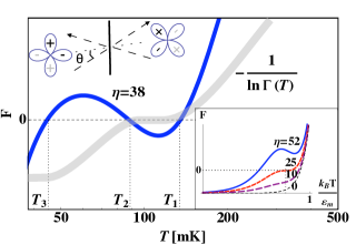
Figure 1: Reentrance effect in MQT. Sketch of temperature dependence of decay rate (wide shadow line) illustrates the effect featuring three transitions between thermal activation and MQT regimes. Experimental transition temperatures are given by zeros of function $F(x)$, defined in the text (blue line) for $\eta=38$. Lower inset shows development of non-monotonic feature of function $F(x)$ with increasing $\eta$, at $\eta>25$. Upper inset illustrates junction geometry and scattering electron trajectory (dashed line).

Nonlinear resonance Josephson dynamics. To investigate the real time Josephson dynamics, one needs to generalize our approach to non-equilibrium states. This is done by considering the partition function defined through the action on the real time Keldysh contour Zaikin1990 . Then proceeding, as before, by introducing the instantaneous basis, we derive the equation for the Keldysh-Green’s functions, $\hat{G}^{ab}$, $[i\partial_{t}-\hat{H}(\varphi^{a},\dot{\varphi}^{a})]\hat{G}^{ab}(t-t^{\prime})=a\delta^{ab}\delta(t-t^{\prime})$, with the same Hamiltonian as in Eq. (1), here $a,b=\pm$ label the forward and backward branches of the Keldysh contour. The semiclassical dynamics of the superconducting phase is given by the least action principle, $(\delta/\delta\chi)S_{\text{eff}}[\varphi,\chi]_{\chi=0}=0$, formulated in terms of the Wigner variables, $\varphi^{a}=\varphi+a\chi/2$ Kamenev2005 . Calculating the functional derivative, we get,

$${C\over 2e}\,\ddot{\varphi}+\text{Tr}\left(\hat{I}_{J}\hat{\rho}\right)={I_{e}},\quad\hat{I}_{J}=2e(\partial_{\varphi}\hat{E}+i[\hat{E},\hat{\mathcal{A}}]).$$ (6)

Here $\hat{\rho}(t)=(1/2i)\sum_{a}\hat{G}^{aa}(t,t)$ is the non-equilibrium single particle density matrix, which satisfies, by virtue of the equation for $\hat{G}^{ab}$, the Liouville equation,

$$i\dot{\hat{\rho}}=[\hat{H}\,,\,\hat{\rho}],\quad\hat{H}=\hat{E}-\dot{\varphi}\hat{\mathcal{A}}.$$ (7)

Eqs. (6) and (7) are exact in the semiclassical limit, and give a general description of the non-adiabatic Josephson dynamics in all kinds of junctions. These equations constitute another main result of this paper.

For the MGS pairs, Eq. (7) reduces to the Bloch equation for the two-level density matrix parameterized with the angle $\theta$. In this case, Eqs. (6), (7) become analogous to the ones describing electromagnetic modes in a cavity embedded in a medium of two-level atoms Eberly . The most interesting is the case of the resonant excitation of the MGS pairs, which corresponds to the Josephson plasma frequency lying within the MGS band, $\omega_{p}<\varepsilon_{m}$. Suppose a small oscillating biasing current is applied to the junction, $I_{e}\cos\omega t$, with frequency slightly detuned from the plasma frequency, $\delta=\omega-\omega_{p}\ll\omega$. The resonant dynamics of the superconducting phase, $\varphi(t)=\text{Re}(\varphi_{\omega}e^{-i\omega t})$, is described by the averaged equation for slow varying complex amplitude, $\varphi_{\omega}(t)$,

$$-2i\dot{\varphi}_{\omega}+\left[-2\delta+\gamma(r)\right]\varphi_{\omega}=eI_{e}/\omega_{p}C,$$ (8)

where $\gamma=\gamma^{\prime}+i\gamma^{\prime\prime}$ is the nonlinear MGS response,

$$\gamma^{\prime}(r)=\gamma_{0}^{\prime}+\partial^{2}_{\varphi}\bar{\varepsilon}{\gamma^{\prime\prime}\over\Gamma_{1}}\,r^{2},\;\gamma^{\prime\prime}(r)\!=\!\frac{\Gamma\gamma_{0}^{\prime\prime}}{\sqrt{(r\bar{A}\omega)^{2}+\Gamma^{2}}}$$ (9)

(the nonlinear adiabatic term is dropped from Eq. (8) to emphasize the MGS effect). In Eq. (9) the bar indicates the resonant values, $r=|\varphi_{\omega}|$, and the quantity $\gamma_{0}$ refers to the linear MGS response given by the analytical continuation of Eq. (4) to real frequencies, $i\nu\rightarrow\omega+i0$. The response is calculated (see Appendix) by solving the Bloch equation (7) assuming the MGS adiabatically following, in the rotating frame, the evolution of the phase amplitude, and adding small decoherence rates $\Gamma_{1},\Gamma_{2}\ll\varepsilon_{m}$. The MGS decoherence is induced, e.g., by scattering to the itinerant nodal states by the facet edges or other rare inhomogeneities, leading to the MGS intrinsic broadening, $\Gamma=\sqrt{\Gamma_{1}\Gamma_{2}}$. The dissipative part of the linear response is estimated,

$$\gamma_{0}^{\prime\prime}(\omega,T)\sim{\omega\over\varepsilon_{m}R_{n}C}\tanh{\omega\over 4T}.$$ (10)

It gives the frequency independent quality factor at zero temperature, $Q_{MGS}=\omega/\gamma_{0}^{\prime\prime}\sim\varepsilon_{m}R_{n}C$. It is instructive to compare this result to the damping effect of the nodal quasiparticles, $Q_{nodal}\sim\Delta_{0}R_{n}C\gg Q_{MGS}$, see Appendix (cf. Bruder1995 ; Barash1995 ; Kawabata2005 ).

Equation (9) provides an extension of the linear response equation (4) to the nonlinear region, when the Rabi frequency of MGS transitions exceeds the MGS intrinsic width, $r\bar{A}\omega\gtrsim\Gamma$. In this nonlinear regime relevant for narrow MGS levels the stationary response amplitude as function of detuning is defined by relation,

$$\delta=\frac{1}{2}\gamma^{\prime}(r)\pm\frac{1}{2r}\sqrt{(e{I}_{e}/C\omega_{p})^{2}-[\gamma^{\prime\prime}(r)r]^{2}}.$$ (11)

The response demonstrates the bifurcation regime shown in Fig. 2, which is typical for nonlinear oscillators, but here is entirely controlled by MGS characteristics rather than adiabatic Josephson potential. The bifurcation appears at very small driving currents, $\tilde{I}_{e}=(I_{e}/2I_{C})Q_{MGS}\sim\Gamma/\omega\bar{A}\ll 1$. The most striking feature of the response is the explosive growth of the peak amplitude, $r_{max}=\tilde{I}_{e}[1-(\tilde{I}_{e}/I_{e}^{\ast})^{2}]^{-1/2}$, for the driving current approaching the value $I_{e}^{\ast}=\Gamma/\omega\bar{A}$. This effect is caused by the MGS saturation at large driving amplitudes, which is manifested by decreasing damping in equation (9). The divergency is smeared by adding small damping, e.g., by nodal quasiparticles, and changes to a steep dependence asymptotically approaching the line, $r_{max}=(\tilde{I}_{e}-I_{e}^{\ast})(Q_{nod}/Q_{MGS})$. The Rabi dynamics of the MGS should be more clearly exposed in the time resolved experiments.

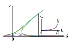
Figure 2: Effect of MGS on nonlinear resonance response of the junction. Response amplitude as function of detuning is shown for different amplitudes of driving current. Inset: maximum response amplitude as a function of driving current, dots indicate current values in the main figure.

In conclusion, we considered the effects of midgap states on Josephson dynamics in d-wave superconducting junctions. The analysis is based on the developed general theoretical framework for non-adiabatic Josephson dynamics in junctions containing low energy quasiparticles. We identified a reentrance effect in MQT, and connected that to the experimental observations. We also investigated the nonlinear dynamical response of the junction caused by coupling to nonlinear MGS dynamics. By analyzing the experiment Bauch2005 in terms of the interaction with MGS, we found that the MGS bandwidth in the experimental junction is smaller than the Josephson plasma frequency, $\varepsilon_{m}<\omega_{p}$. This implies that the resonance condition for MGS excitation is not fulfilled, and MGS should not affect the real time junction dynamics, which thus would be similar to conventional Josephson oscillators. The quality factor is then defined by the nodal quasiparticles, and is estimated from the experimental data, $Q_{nod}\sim(\Delta_{0}/\omega_{p})^{2}\sim 40$. In order to increase this factor the strategy would be to increase the ratio, $\Delta_{0}/\omega_{p}$, which is, however, impossible beyond the limit, $Q_{nod}\sim 1/D$, provided MGS remain off-resonance ($\varepsilon_{m}\sim\sqrt{D}\Delta_{0}<\omega_{p}$). Exceeding this limit necessarily implies resonant excitation of the MGS, and establishing the nonlinear regime described in this paper.

Acknowledgement. We are thankful to J. Clark, M. Fogelström, T. Löfwander, and C. Tsuei for useful discussions; illuminative discussion of experiment with Th. Bauch and F. Lombardi are gratefully acknowledged. The work was supported by the Swedish Research Council (VR), and the European FP7-ICT Project MIDAS.

Appendix A Appendix

In this appendix we present details of the derivation of (a) effective action for superconducting phase, multiple critical temperatures for transitions between thermal activation and MQT regimes under interaction with MGS; (b) MGS energy spectrum and transition matrix elements, MGS linear response and comparison to the damping effect of nodal quasiparticles; and (c) the nonlinear junction dynamics under resonant interaction with MGS.

Appendix B Reentrance effect in MQT

In this section we derive the dispersion equation for small phase fluctuation in imaginary time used to evaluate the crossover temperature between thermal activation and MQT decay of persistent Josephson current. To this end we shall also need to derive equations defining the MGS characteristics: energy dispersion equation, and interlevel matrix elements, and discuss MGS general properties, and present some explicit analytical equations.

B.1 Imaginary time approach

Starting from the imaginary time representation of partition function and performing integration over the fermionic fields, one obtains the equilibrium partition function as a path integral over the phase with an euclidian effective action $S_{E}^{\text{eff}}$,

$$Z=\int\mathcal{D}\varphi e^{-S_{E}^{\text{eff}}[\varphi]},\qquad S_{E}^{\text{eff}}[\varphi]=\int_{0}^{\beta}d\tau\left[\frac{C}{8e^{2}}\dot{\varphi}^{2}+U_{\text{ext}}(\varphi)\right]-\text{Sp}\ln\hat{G}^{-1},$$ (12)

where $U_{\text{ext}}(\varphi)=-(I_{\text{e}}/2e)\varphi$ is an inductive energy of a biasing current $I_{e}$, and

$$\hat{G}^{-1}_{ij}=\Bigl{(}\partial_{\tau}+\hat{H}_{ij}(\varphi,\dot{\varphi})\Bigr{)},\qquad\hat{H}_{ij}=\delta_{ij}E_{i}-i\dot{\varphi}\mathcal{A}_{ij}.$$ (13)

The matrix $\hat{E}$ in this equation is constructed with the eigen energies, $E_{ij}=E_{i}\delta_{ij}$ of the microscopic junction Hamiltonian,

$$\mathcal{H}\phi_{i}=E_{i}\phi_{i},$$ (14)

$$\mathcal{H}=\left[\frac{(-i\mathbf{\nabla})^{2}}{2m}-\mu+V\right]\sigma_{z}+\hat{\Delta}e^{i\chi}\sigma_{+}+\hat{\Delta}e^{-i\chi}\sigma_{-},$$ (15)

where $\hat{\Delta}$ denotes a non-local operator, $\hat{\Delta}\phi\equiv\int d\mathbf{r}^{\prime}\Delta(\mathbf{r},\mathbf{r}^{\prime})\phi(\mathbf{r}^{\prime})=\int d\mathbf{k}\,\Delta(\mathbf{k},\mathbf{r})\int d\mathbf{R}\,\phi(\mathbf{r}+\mathbf{R})e^{i\mathbf{k}\cdot\mathbf{R}}$, and

$$\chi(\mathbf{r})\equiv\begin{cases}\frac{\varphi}{2},\ &\mathbf{r}\in L\\ -\frac{\varphi}{2},\ &\mathbf{r}\in R\end{cases},$$ (16)

denotes the phase of the order parameter in the left ($L$) and right ($R$) electrodes; $V(\mathbf{r})$ represents an interface potential.

The matrix of operator $\mathcal{\hat{A}}$ is constructed with the matrix elements of the transition between the basis states, Eq. (14),

$$\mathcal{A}_{ij}=(\phi_{i},\left[i\partial_{\varphi}-(1/4)\sigma_{z}\mathrm{sign}(x)\right]\phi_{j}).$$ (17)

An alternative representation of this matrix is given through the relation to the matrix $I_{ij}=(\phi_{i},\,\hat{I}_{J}\,\phi_{j})$,

$$i\mathcal{A}_{ij}=\frac{1}{2e}\frac{I_{ij}}{\varepsilon_{ij}},\qquad i\neq j,$$ (18)

where $\varepsilon_{ij}=E_{i}-E_{j}$. As it is shown in the next section, this matrix represents the Josephson current flowing through the junction, and is connected to the current density operator via equations,

$$I_{ij}=\int_{S}d\mathbf{n}\cdot\mathbf{j}_{ij}(\mathbf{r}),$$

$$\mathbf{j}_{ij}(\mathbf{r})=\frac{e}{2m}\left.(i\mathbf{\nabla}-i\mathbf{\nabla}^{\prime})\phi_{i}^{\dagger}(\mathbf{r})\phi_{j}(\mathbf{r}^{\prime})\right|_{\mathbf{r}=\mathbf{r^{\prime}}}.$$ (19)

B.2 Current operator

Here we present a proof for the interpretation of $\hat{I}_{J}$ as the quantum mechanical current operator. To do so we identify the current density operator as

$$\mathbf{j}_{ij}(\mathbf{r})=\frac{e}{2m}\left.(i\mathbf{\nabla}-i\mathbf{\nabla}^{\prime})\phi_{i}^{\dagger}(\mathbf{r})\phi_{j}(\mathbf{r}^{\prime})\right|_{\mathbf{r}=\mathbf{r^{\prime}}}.$$ (20)

The current through the interface, $S$, is given by

$$I_{ij}=\int_{S}d\mathbf{n}\cdot\mathbf{j}_{ij}(\mathbf{r}).$$

If we consider the system as an infinitely large loop we can use the fact that no current is flowing through any other part of the surface of the superconductor so we may extend the surface $S$ around the whole superconductor and use Gauss law:

$$2I_{ij}=\int_{\mathbf{r}\in L}dV\ \mathbf{\nabla}\cdot\mathbf{j}_{ij}(\mathbf{r})-\int_{\mathbf{r}\in R}dV\ \mathbf{\nabla}\cdot\mathbf{j}_{ij}(\mathbf{r}).$$ (21)

From the explicit form of the BdG Hamiltonian (15) one finds the relations,

$$\begin{split}(-i\mathbf{\nabla})\cdot\mathbf{j}_{ij}(\mathbf{r})&=-\frac{e}{2m}\left[[-\nabla^{2}\phi_{i}(\mathbf{r})]^{\dagger}\phi_{j}(\mathbf{r})-\phi_{i}^{\dagger}(\mathbf{r})[-\nabla^{2}\phi_{j}(\mathbf{r})]\right]\\ &=-e\left[(E_{i}-E_{j})\phi_{i}^{\dagger}(\mathbf{r})\sigma_{z}\phi_{j}(\mathbf{r})+\phi^{\dagger}_{i}(\mathbf{r})[\mathcal{H},\sigma_{z}]\phi_{j}(\mathbf{r})\right].\\ \end{split}$$ (22)

The last term (the commutator between the ”charge operator” $\sigma_{z}$, and the quasiparticle Hamiltonian) can be rewritten as

$$[\sigma_{z},\mathcal{H}]=2i\partial_{\chi}\mathcal{H}=\begin{cases}4i\partial_{\varphi}\mathcal{H},\ &\mathbf{r}\in L\\ -4i\partial_{\varphi}\mathcal{H},\ &\mathbf{r}\in R\\ \end{cases}.$$ (23)

The current operator then becomes

$$I_{ij}=(-i)2e\left[(\phi_{i},i\partial_{\varphi}\mathcal{H}\phi_{j})-(E_{j}-E_{i})\frac{1}{4}(\phi_{i},\mathrm{sign}(x)\sigma_{z}\phi_{j})\right].$$ (24)

By differentiating the eigenvalue equation $\mathcal{H}\phi_{i}=E_{i}\phi_{i}$ wrt $\varphi$ one obtains the following identities:

$$\begin{split}&(\phi_{i},i\partial_{\varphi}\mathcal{H}\phi_{i})=i\partial_{\varphi}E_{i},\\ &(\phi_{i},i\partial_{\varphi}\mathcal{H}\phi_{j})=(E_{j}-E_{i})(\phi_{i},i\partial_{\varphi}\phi_{j}),\quad i\neq j\end{split}.$$ (25)

From this one sees that the current matrix elements are given by

$$\begin{split}I_{ii}&=2e\partial_{\varphi}E_{i},\\ I_{ij}&=2ei(E_{i}-E_{j})\mathcal{A}_{ij},\end{split}$$ (26)

or in explicit matrix form

$$\hat{I}=2e\left(\partial_{\varphi}\hat{E}+i[\hat{E},\hat{A}]\right).$$ (27)

B.3 Quasiclassical wave functions

In this subsection we sketch the quasiclassical formalism used for the evaluation of the MGS properties.

Consider an interface with normal, $\hat{\mathbf{n}}$, pointing in the positive $x$ direction ($\hat{\mathbf{n}}\cdot\hat{\mathbf{x}}>0$). The incident angle, $\theta$, of an electronic trajectory is defined through the relation

$$k_{F}\cos\theta=\mathbf{k}_{F}\cdot\mathbf{n}.$$

The d-wave order parameter is aligned with the crystal a-b axes according to $\Delta_{0}(k_{a}^{2}-k_{b}^{2})$ where $k_{a}=\hat{\mathbf{k}}_{F}\cdot\hat{\mathbf{a}}$, $k_{b}=\hat{\mathbf{k}}_{F}\cdot\hat{\mathbf{b}}$. Introducing the misorientation angle $\alpha:$ $\mathbf{n}\cdot\mathbf{a}=\cos\alpha$ and $\mathbf{n}\cdot\mathbf{b}=\sin\alpha$ we can write $k_{a}=\cos(\alpha-\theta)$ and $k_{b}=\sin(\alpha-\theta)$. The order parameter can then be written as a function of the two angles $\alpha,\theta$:

$$\Delta(\theta)=\Delta_{0}\cos 2(\alpha-\theta).$$ (28)

Assuming specular reflection, the momentum parallel to the interface is conserved upon reflection, while the perpendicular momentum is inverted, (or equivalently, the reflected angle is given by $\pi-\theta$). The quasiclassical wave functions have the form of linear combinations of plane waves

$$\phi(\mathbf{r},\mathbf{k}_{F||})=\frac{1}{\sqrt{S}}e^{i\mathbf{k}_{F||}\cdot\mathbf{r}_{||}}\sum_{\sigma=\pm}\tilde{\phi}^{\sigma}(x)e^{i\mathbf{k}_{F}^{\sigma}\cdot\mathbf{n}x},$$ (29)

where $\mathbf{r}=x\mathbf{n}+\mathbf{r}_{||}$, $\mathbf{k}_{F}^{\sigma}=\sigma\mathbf{k}_{F\perp}+\mathbf{k}_{F||}$, and $S$ is the interface area. The slowly varying envelopes, $\tilde{\phi}^{\sigma}(x)$, satisfy the quasiclassical BdG equations,

$$\left[\mathbf{v}^{\sigma}_{F}\cdot\mathbf{n}(-i\partial_{x})\sigma_{z}+\Delta_{j}^{\sigma}e^{i\chi}\sigma_{+}+\Delta_{j}^{\sigma}e^{-i\chi}\sigma_{-}\right]\tilde{\phi}^{\sigma}(x)=E\tilde{\phi}^{\sigma}(x),\quad j=\begin{cases}L,\quad x<0\\ R,\quad x>0\end{cases},$$ (30)

where the shorthand notation is introduced, $\Delta_{j}^{\sigma}=\Delta_{0}\cos 2\left(\sigma\theta-\alpha_{j}\right),$ and $\alpha_{j=L,R}$ denote the angles of the a-b crystal axes to the normal of the interface, $\hbar=1$. It is convenient to incorporate the sign of the order parameter into the phase,

$$\varphi_{j}^{\sigma}=\begin{cases}\varphi/2+\Theta(-\Delta_{L}^{\sigma})\pi,\quad&j=L\\ -\varphi/2-\Theta(-\Delta_{R}^{\sigma})\pi,\quad&j=R\end{cases}.$$ (31)

The local interface potential is replaced in the quasiclassical approximation with the boundary conditions for slow wave functions envelops,

$$\phi^{\sigma}(0^{-})=T^{\sigma\sigma^{\prime}}\phi^{\sigma^{\prime}}(0^{+}),$$ (32)

where $T^{\sigma\sigma^{\prime}}$ denotes a general single channel (i.e. for given trajectory) transfer matrix, characterized by the transmission amplitude, $d(\theta)$, and reflection amplitude $r(\theta)$, ($|r|^{2}+|d|^{2}=1$).

B.4 MGS spectrum and transition matrix elements

Here we derive equations defining the MGS energy spectrum and transition matrix elements for planar junctions with specular interfaces.

The bound state solutions to equation (30) have the general form,

$$\tilde{\phi}^{\sigma}(x)=\begin{cases}A^{\sigma}u_{L}^{\sigma}e^{-\zeta_{L}^{\sigma}|\tilde{x}|},\quad x<0\\ B^{\sigma}u_{R}^{\sigma}e^{-\zeta_{R}^{\sigma}|\tilde{x}|},\quad x>0\end{cases},$$ (33)

where

$$u^{\sigma}_{j}=\frac{1}{\sqrt{2}}\begin{pmatrix}e^{-i\gamma_{j}^{\sigma}}\\ e^{i\gamma_{j}^{\sigma}}\end{pmatrix},\quad\zeta_{j}^{\sigma}=\frac{|\Delta_{j}^{\sigma}|}{|\mathbf{v}_{F}^{\sigma}\cdot\mathbf{n}|}\sin\eta_{j}^{\sigma},\quad j=L,R,$$ (34)

and $\gamma_{j}^{\sigma}=\sigma\eta_{j}^{\sigma}+\varphi_{j}^{\sigma}/2$ with

$$2\eta_{j}^{\sigma}=\begin{cases}\text{acos}(E/|\Delta_{l}^{\sigma}|),\quad j=L\\ -\text{acos}(E/|\Delta_{r}^{\sigma}|),\quad j=R\end{cases}.$$ (35)

Using the properties of the spinors, the matching condition Eq. (32) can be rewritten into two sets of equations $A^{\sigma}=\mathcal{N}^{\sigma\sigma^{\prime}}B^{\sigma^{\prime}}$, $0=\mathcal{M}^{\sigma\sigma^{\prime}}B^{\sigma^{\prime}}$ where $\mathcal{N}^{\sigma\sigma^{\prime}}=T^{\sigma\sigma^{\prime}}\cos\left(\gamma_{L}^{\sigma}-\gamma_{R}^{\sigma^{\prime}}\right),\ \mathcal{M}^{\sigma\sigma^{\prime}}=T^{\sigma\sigma^{\prime}}i\sin\left(\gamma_{L}^{\sigma}-\gamma_{R}^{\sigma^{\prime}}\right)$, determining the coefficients, $A^{\sigma}$, and, $B^{\sigma}$, upto a normalization constant. The condition that these equations have non-trivial solutions, $\text{det}\mathcal{M}=0$, defines the spectral equation,

$$\prod_{\sigma=\pm}\sin\left[\gamma_{L}^{\sigma}(E)-\gamma_{R}^{\sigma}(E)\right]=R\prod_{\sigma=\pm}\sin\left[\gamma_{L}^{\sigma}(E)-\gamma_{R}^{-\sigma}(E)\right].$$ (36)

where $R=|r|^{2}=1-D$.

To obtain an expression for the transition matrix elements, $\mathcal{A}_{12}$, we make use of the relationship with the current matrix elements in Eq. (18),

$$\mathcal{A}\equiv i\mathcal{A}_{12}=\frac{1}{2e}\frac{I_{12}}{(E_{1}-E_{2})},$$

where the current matrix elements are given by Eq. (20) within the quasiclassical approximation,

$$I_{12}=e\sum_{\sigma=\pm}\left.(\mathbf{v}_{F}^{\sigma}\cdot\mathbf{n})(\tilde{\phi}^{\sigma}_{1})^{\dagger}\tilde{\phi}_{2}^{\sigma}\right|_{x=0}=e\sum_{\sigma=\pm}(\mathbf{v}_{F}^{\sigma}\cdot\mathbf{n})[B^{\sigma}_{1}]^{*}B^{\sigma}_{2}\cos\left[\eta^{\sigma}_{R}(E_{1})-\eta^{\sigma}_{R}(E_{2})\right].$$ (37)

B.5 Selection rule

For a junction with $\frac{\pi}{4}/\frac{\pi}{4}$ orientation, there exists a symmetry relation, $\Delta_{L}^{\sigma}=\Delta_{R}^{\sigma}\equiv\Delta_{\frac{\pi}{4}}$, and consequently, $\eta_{L}^{\sigma}=-\eta_{R}^{\sigma}\equiv\eta_{\frac{\pi}{4}}=(1/2)\text{acos}(E/\Delta_{\frac{\pi}{4}})$. The spectral equation then simplifies,

$$\cos^{2}(2\eta_{\frac{\pi}{4}})=D\cos^{2}(\varphi/2),$$ (38)

and has the two solutions $E_{1}=-E_{2}=\sqrt{D}\Delta_{\frac{\pi}{4}}\cos(\varphi/2)$. For a spatially symmetric potential, the amplitudes in Eq. (33) are given by equations (upto normalization factor ensuring that $(\phi,\phi)=1$),

$$B^{+}_{1,2} =\sqrt{R}\cos(\varphi/2),\quad A^{+}_{1,2} =\pm\sqrt{R}\cos(\varphi/2)$$ (39)

$$B^{-}_{1,2} =\sin(2\eta_{\frac{\pi}{4}}(E_{1,2})+\varphi/2),\quad A^{-}_{1,2} =\pm\sin(2\eta_{\frac{\pi}{4}}(E_{1,2})+\varphi/2)$$

Inserting these amplitudes into equation (37) for the current matrix element (which is proportional to $\mathcal{A}$), we arrive at the important result,

$$\mathcal{A}=0.$$

Now we show that this result is a particular case of a general selection rule forbidding transitions among the MGS for any symmetric junction. This selection rule is imposed by the symmetry of the Hamiltonian, Eq. (15), under charge and parity conjugation $\mathcal{CP}$,

$$\mathcal{CP}\phi(\mathbf{r})=\phi^{*}(-\mathbf{r}).$$

To prove our statement we first note that the $\mathcal{C}\mathcal{P}$-symmetry splits the Hilbert space of the Hamiltonian (15), into two subspaces which correspond to the even and odd transformations of the eigen states under $\mathcal{C}\mathcal{P}$ conjugation,

$$\mathcal{CP}\phi_{i}=\pm\phi_{i}.$$

Then we find that the operator that defines the transition matrix elements, $\mathcal{A}=i\mathcal{A}_{12}=-(\phi_{1},[\partial_{\varphi}+(i/4)\text{sign}(x)\sigma_{z}]\phi_{2})$, respects the $\mathcal{C}\mathcal{P}$-symmetry, and therefore the matrix elements between the states belonging to the odd-subspace and even-subspace vanish.

Next, we notice that an arbitrary symmetric junction is obtained by continuous rotation of the ${\pi\over 4}/{\pi\over 4}$ junction. Such a rotation preserves the $\mathcal{C}\mathcal{P}$-symmetry, and the eigen functions transform smoothly under the rotation, unless the nodes of the order parameter are crossed. Therefore, the wave functions initially belonging to different discrete subspaces of the symmetry operator will maintain this property during the rotation. Inspection of Eqs. (33) and (39) for the ${\pi\over 4}/{\pi\over 4}$ junction proves that indeed the two MGS eigen functions obtain opposite signs under $\mathcal{C}\mathcal{P}$ transformation, and thus belong to different subspaces of the symmetry operator.

This proves that the transition matrix elements will equal zero for the MGS of all symmetric junctions.

B.6 $\frac{\pi}{4}+\kappa/\frac{\pi}{4}-\kappa$ orientations

The antisymmetric orientation is one of the few orientations for which one can obtain non-trivial analytical solutions $\mathcal{A}$. For these orientations the symmetry holds,

$$|\Delta_{L}^{\pm}|=|\Delta_{R}^{\mp}|\equiv\Delta^{\pm}.$$ (40)

For trajectories that admit a pair of MGS we find the spectral equation,

$$\cos^{2}(\eta^{+}+\eta^{-})=D\cos^{2}\varphi/2.$$ (41)

where the shorthand $\eta^{\pm}=\eta_{L}^{\pm}=-\eta_{R}^{\mp}$ was introduced for notational convenience. Using the definitions, $\cos 2\eta^{\pm}=E/|\Delta^{\pm}|$, and $\sin 2\eta^{\pm}=\sqrt{1-E^{2}/|\Delta^{\pm}|^{2}}$, we find the solution,

$$E=\pm|\Delta^{+}\Delta^{-}|\sqrt{D}\cos\frac{\varphi}{2}\frac{2\sqrt{1-D\cos^{2}\frac{\varphi}{2}}}{\sqrt{(|\Delta^{+}|+|\Delta^{-}|)^{2}-4|\Delta^{+}\Delta^{-}|D\cos^{2}\frac{\varphi}{2}}}.$$ (42)

Once an analytical expression for the spectrum has been found one can also obtain an analytic expression for $\mathcal{A}$ in terms of $\eta^{\pm}$,

$$\mathcal{A}_{12}=\sqrt{R}\frac{(\sin 2\eta^{+}-\sin 2\eta^{-})}{2E\sin\left(\eta^{+}+\eta^{-}\right)}\left(\frac{|\Delta^{+}\Delta^{-}|\sin 2\eta^{+}\sin 2\eta^{-}}{|\Delta^{+}|\sin 2\eta^{+}+|\Delta^{-}|\sin 2\eta^{-}}\right).$$ (43)

Here $\eta^{\pm}=(1/2)\arccos(E/|\Delta^{\pm}|)$ with the energy given by Eq. (42).

Notice that for $\kappa=0$, we have $\eta^{+}=\eta^{-}$, so that the matrix element vanishes for this orientation, as also shown above. For small misorientation, $\kappa\ll 1$, this expression can be expanded into

$$\mathcal{A}_{12}\approx\frac{\sqrt{RD}\cos\frac{\varphi}{2}}{\sqrt{1-D\cos^{2}\frac{\varphi}{2}}}\frac{\delta\Delta}{\Delta},$$ (44)

where $\delta\Delta(\theta)=\Delta^{+}(\theta)-\Delta_{0}\sin 2\theta\approx 2\kappa\Delta_{0}\cos 2\theta$. This equation reduces at small transparency,

$$\mathcal{A}_{12}\approx\sqrt{D}\cos\frac{\varphi}{2}\frac{\delta\Delta}{\Delta}\approx 2\kappa\sqrt{D}\cot(2\theta).$$ (45)

B.7 Transition temperature

The decay of the persistent Josephson current at large bias current applied to the junction is represented by escape of a fictitious particle representing the junction from a metastable potential well of the ”washboard potential” formed by the periodic Josephson potential, $U_{J}(\varphi)$, and potential of the current bias, $U_{\text{ext}}(\varphi)=-(I_{e}/2e)\varphi$. Grabert and Weiss Grabert1984 devised a method for direct calculation of a critical temperature of transition from the thermally activated escape to the escape via MQT by analyzing small fluctuations around the saddle point located at the barrier top, $\varphi_{b}$. The semiclassical euclidian action is expanded to second order in the deviation, $\delta\varphi=\varphi-\varphi_{b}$,

$$\begin{split}S_{E}^{\text{eff}}[\varphi]&\approx S^{(0)}[\varphi_{b}]+S_{E}^{(2)}[\delta\varphi],\\ S_{E}^{(2)}&=\int_{0}^{\beta}d\tau\int_{0}^{\beta}d\tau^{\prime}\delta\varphi(\tau)\Lambda(\tau-\tau^{\prime})\delta\varphi(\tau^{\prime})\\ &=\sum_{n}\Lambda(i\omega_{n})|\varphi_{n}|^{2}.\end{split}$$ (46)

The Fourier components, $\Lambda(i\nu_{n})$, of the fluctuation kernel, $\Lambda(\tau-\tau^{\prime})$, with Matsubara frequencies, $\nu_{n}=2\pi n/\beta$, are then the eigenvalues associated with the gaussian fluctuations around the stationary point, $\varphi_{b}$. In the thermal activation regime, the stationary point is stable, and all the eigenvalues are positive, $\Lambda(i\omega_{n})>0$. Transition to the MQT regime is manifested by the instability, indicated by the sign change of the smallest eigenvalue, $\Lambda(i\nu_{1})<0$. The transition temperatures can thus be obtained by finding solutions to the equation, $\Lambda(i\nu_{1})=0$.

To evaluate the fluctuation part of the action for our system we expand in $\delta\varphi$ and keep only second order terms. This gives us,

$$S_{E}^{(2)}[\delta\varphi]=\int_{0}^{\beta}d\tau\left[\frac{C}{8e^{2}}\delta\dot{\varphi}^{2}+\frac{1}{2}\left.\frac{\partial^{2}U_{\text{ext}}}{\partial\varphi^{2}}\right|_{\varphi_{b}}\delta\varphi^{2}\right]+\int^{\beta}_{0}d\tau d\tau^{\prime}\delta\varphi(\tau)K(\tau-\tau^{\prime})\delta\varphi(\tau^{\prime}),$$ (47)

where

$$K(\tau-\tau^{\prime})=\frac{1}{2}\left.\frac{\delta^{2}\text{Sp}\ln\hat{G}^{-1}}{\delta\varphi(\tau)\delta\varphi(\tau^{\prime})}\right|_{\varphi=\varphi_{b}}.$$ (48)

It is convenient to perform the functional differentiation in a basis where the dependence on $\dot{\varphi}$ is removed. This is achieved by a using rotation matrix $U:\partial_{\varphi}U=i\mathcal{A}U$,

$$K(\tau-\tau^{\prime})=\frac{1}{2}\text{Tr}\left(\tilde{\hat{\rho}}(\tau)\frac{\partial^{2}\tilde{\hat{H}}}{\partial\varphi^{2}}(\tau)\right)_{\varphi_{b}}\delta(\tau-\tau^{\prime})+\text{Tr}\left(\tilde{\hat{G}}(\tau,\tau^{\prime})\frac{\partial\tilde{\hat{H}}}{\partial\varphi}(\tau^{\prime})\tilde{\hat{G}}(\tau^{\prime},\tau)\frac{\partial\tilde{\hat{H}}}{\partial\varphi}(\tau)\right)_{\!\varphi_{b}}.$$ (49)

The contribution from the first part combines with the second derivative of the external potential to define the barrier frequency,

$$-\omega_{b}^{2}=\frac{8e^{2}}{C}\left[\frac{1}{2}\frac{\partial^{2}U_{\text{ext}}}{\partial\varphi^{2}}+\frac{1}{2}\text{Tr}\left(\tilde{\hat{\rho}}(\tau)\frac{\partial^{2}\tilde{\hat{H}}}{\partial\varphi^{2}}(\tau)\right)\right]_{\varphi_{b}},$$ (50)

leaving the second part which we denote by small $k(\tau-\tau^{\prime})$:

$$k(\tau-\tau^{\prime})=\frac{1}{(2e)^{2}}\text{Tr}\left(\hat{G}(\tau,\tau^{\prime})\hat{I}_{J}(\tau^{\prime})\hat{G}(\tau^{\prime},\tau)\hat{I}_{J}(\tau)\right)_{\varphi_{b}}.$$ (51)

Here $\hat{I}_{J}$ is the current operator as defined in Eq. (64), the imaginary time (Matsubara) Green function for constant phase ($\varphi(\tau)=\varphi_{b}$) is given by equation,

$$(G_{0})_{ij}(\tau,\tau^{\prime})=-\left[\theta(\tau-\tau^{\prime})(1-\rho_{i}^{0})-\theta(\tau^{\prime}-\tau)\rho_{i}^{0}\right]e^{-E_{i}^{0}(\tau-\tau^{\prime})}\delta_{ij},$$ (52)

where $\rho_{i}^{0}=n_{F}(E_{i}^{0})$, and $E_{i}^{0}=E_{i}(\varphi_{b})$. Due to the boundary condition, $\delta\varphi(0)=\delta\varphi(\beta)$, we can perform integration by parts to obtain,

$$S_{E}^{(2)}[\delta\varphi]=\int_{0}^{\beta}d\tau d\tau^{\prime}\delta\varphi(\tau)\Lambda(\tau-\tau^{\prime})\delta\varphi(\tau^{\prime}),$$ (53)

where

$$\Lambda(\tau-\tau^{\prime})=\frac{C}{8e^{2}}\left[\left(-\partial_{\tau}^{2}-\omega_{b}^{2}\right)\delta(\tau-\tau^{\prime})+\frac{8e^{2}}{C}k(\tau-\tau^{\prime})\right].$$ (54)

The Fourier representation of the operator $\Lambda(\tau-\tau^{\prime})$ defines the eigenvalues,

$$\Lambda(i\nu_{n})=\frac{C}{8e^{2}}\left[-(i\nu_{n})^{2}-\omega_{b}^{2}-i\nu_{n}\gamma_{0}(i\nu_{n})\right],\qquad\nu_{n}=\frac{2\pi n}{\beta},$$ (55)

where $-i\nu_{n}\gamma_{0}(i\nu_{n})=(8e^{2}/C)k(i\nu_{n})$ has the explicit form,

$$\gamma_{0}(i\nu_{n})=\frac{4e^{2}}{C}\sum_{ij}\frac{\varepsilon_{ij}|\mathcal{A}_{ij}|^{2}(\rho_{i}^{0}-\rho_{j}^{0})}{\varepsilon_{ij}-i\nu_{n}}.$$ (56)

Here $\varepsilon_{ij}=E_{i}^{0}-E_{j}^{0}$ and $\mathcal{A}_{ij}=\mathcal{A}_{ij}(\varphi_{b})$. Comparing this result with Eq. (46) we find the equation for the transition temperature to the MQT regime,

$$\Lambda(i\nu_{1})\propto\nu_{1}^{2}-\omega_{b}^{2}-i\nu_{1}\gamma_{0}(i\nu_{1})=0.$$ (57)

B.8 MGS and reentrance effect

The reentrance effect described in the article results from a strong temperature dependence of dissipation produced by the MGS, which decrease with increasing temperature. After truncating to the MGS subspace, we present Eqs. (56) and (57) on the form, dropping the subscript,

$$\begin{split}&\nu^{2}-\omega_{b}^{2}-i\nu\gamma_{0}(i\nu_{1})=0\\ &\Rightarrow\nu^{2}-\nu\frac{4e^{2}S}{C}\sum_{\pm}\left\langle\frac{i\varepsilon\mathcal{A}^{2}\rho_{z}}{\pm\varepsilon-i\nu}\right\rangle=\omega_{b}^{2}\\ &\Rightarrow\nu^{2}\left(1+\frac{8e^{2}S}{C}\left\langle\frac{\varepsilon\mathcal{A}^{2}\rho_{z}}{\varepsilon^{2}+\nu^{2}}\right\rangle\right)=\omega_{b}^{2}.\\ \end{split}$$ (58)

Here $S$ is the junction area, and $\rho_{z}=n_{F}(E_{1})-n_{F}(E_{2})$ while the average $\langle\ldots\rangle$ is defined as

$$\langle\ldots\rangle=\int_{+}\frac{d^{2}\mathbf{k}_{F}}{(2\pi)^{2}}\ldots,$$ (59)

where integration is performed over the Fermi wave vectors in the positive direction of the interface normal. Assuming the interface to be orthogonal to the crystal a-b plane, and taking into account strong anisotropy of the Fermi surface, we write the integral on the form,

$$S\langle\ldots\rangle=N\int_{-\pi/2}^{\pi/2}d\theta\ldots\ldots,$$ (60)

where $N=Sk_{F}/2\pi c$ is the number of conducting channels for a stack 2D planes with spatial period $c$. For the sake of simplicity, we consider almost symmetric MGS spectrum, $E_{1}=-E_{2}=\varepsilon/2$, giving $\rho_{z}(T)=\tanh(\varepsilon/4T)$, and proceed to integration over $\varepsilon$ in the integral over $\theta$, The equation for the crossover temperature then becomes,

$$(2\pi T)^{2}\left(1+\frac{8e^{2}}{C}N\int_{0}^{\varepsilon_{m}}d\varepsilon g(\varepsilon)\frac{\varepsilon\mathcal{A}^{2}(\varepsilon)\tanh(\varepsilon/4T)}{\varepsilon^{2}+(2\pi T)^{2}}\right)=\omega_{b}^{2}.$$ (61)

where $g(\varepsilon)=4d\theta/d\varepsilon$ is the MGS spectral density. The important qualitative features of the integral, independent of junction geometry, are the saturation effect due to the MGS population number, $\tanh(\varepsilon/4T)$, and the resonance feature in the denominator, $\varepsilon^{2}+(2\pi T)^{2}$. Numerical studies show that these features define the temperature dependence of the integral, while the role of the function, $g(\varepsilon)\varepsilon\mathcal{A}^{2}(\varepsilon)$, which contains information about junction geometry, is qualitatively insignificant. This observation allows us to approximate the latter with some constant whose magnitude is set by $\mathcal{A}^{2}\sim D$, because $g(\varepsilon)\sim 1/\varepsilon_{m}$, and $\varepsilon\sim\varepsilon_{m}$;

$$g(\varepsilon)\varepsilon\mathcal{A}^{2}(\varepsilon)=a\int_{-\pi/2}^{\pi/2}d\theta D(\theta),$$ (62)

where $a$ is a geometry dependent numerical constant of order $\sim 1$. We are then able to formulate a simple model equation defining the transition temperature,

$$(2\pi T)^{2}\left(1+\frac{8\pi a}{R_{n}C}\int_{0}^{\varepsilon_{m}}d\varepsilon\frac{\tanh(\varepsilon/4T)}{\varepsilon^{2}+(2\pi T)^{2}}\right)=\omega_{b}^{2},$$ (63)

where $R_{n}=\pi/e^{2}S\langle D\rangle$ is the normal junction resistance.

B.9 Fitting MQT transition temperatures

Here we shall outline the method used to fit the transition temperatures in our model to the experiment in Bauch2006 . For this procedure, Eq. (63) will be our model. Before proceeding we first simplify our notation in Eq. (63) by writing $\gamma_{0}(i\nu)=i\nu\eta f(\nu/\varepsilon_{m})$, with $f(x)=\int_{0}^{1}dy\tanh(\pi y/2x)(x^{2}+y^{2})^{-1}$, where $\eta=8a\pi/R_{n}C\varepsilon_{m}$ is the coupling strength. The next, crucial step is to consider a dimensionless function, $F(x,\eta)=x^{2}(1+\eta f(x))$, where $x=2\pi T/\varepsilon_{m}$, and choose the scaling parameter $\varepsilon_{m}$ such that the three argument values, corresponding to given transition temperatures, $T_{1},\,T_{2}$, and $T_{3}$ give the same function value, $F(x_{1},\eta)=F(x_{2},\eta)=F(x_{3},\eta)$; this can only be achieved by adjusting simultaneously the shape of the function $F(x,\eta)$ by tuning parameter $\eta$. This procedure gives unique values for both parameters. Then the barrier frequency is determined by equating, $\omega_{b}^{2}=\varepsilon_{m}^{2}F(x_{1},\eta)$.

It should be noted that in our analysis we have neglected the temperature dependence of the adiabatic Josephson potential. In general the saturation of the MGS may lead to strong temperature dependence of the Josephson current - a feature suggested in Bauch2005 to be the origin of the hump structure. The model was that the potential barrier height changes between two asymptotically temperature independent values over a narrow region 100 mK $<T<$ 150 mK, assumed to still be in the thermally activated regime. The temperature dispersion of the decay rate corresponding to the two different barrier heights is indicated in their Fig. 2b by two shifted lines. This explanation was consistent with an MQT crossover temperature $T^{*}=50$ mK obtained from the plasma frequency with estimated junction capacitance $C=1$ pF. Later experimentsBauch2006 , however, suggested that this value of the junction capacitance was overestimated due to the presence of a stray capacitance originating from the STO substrate. Comparison with typical grain boundary junctions would suggest a junction capacitance of the order of 100 fF, thus increasing the crossover temperature to values right around the anomalous features of the temperature dispersion of the decay rate. Therefore, while the mechanism suggested in Bauch2005 could produce a feature like the one observed in their experiments, the parameters of this particular junction suggest that the reentrance effect discussed in the present paper may be more relevant.

In addition to the stray capacitance from the substrate it was arguedBauch2006 that the c-axis transport in the tilted junction may cause a stray inductance. We can include the effect of such a stray $LC$ oscillator in our analysis by adding an extra term, $\lambda x^{2}/(x^{2}+\tilde{\omega}_{0}^{2})$, to the function $F(x,\eta)$, where $\tilde{\omega}_{0}=\hbar\omega_{0}/\varepsilon_{m}$ is the dimensionless frequency of the stray oscillator, and $\lambda=\hbar^{2}/L_{0}C\varepsilon_{m}^{2}$ is the coupling containing the stray inductance and (unknown) capacitance $C$ of the junction. The latter is connected to the barrier frequency through the relations, $\omega_{b}=\omega_{p}(1-(I_{e}/I_{C})^{2})^{1/4}$, and $\omega_{p}=2eI_{C}/\hbar C$, and evaluated through an iteration procedure, assuming switching current $I_{e}\approx 0.9I_{C}=1.26\,\mu$A. Including the $LC$ oscillator does not produce any qualitative changes but rather slightly modifies numerical values of the fitting parameters. The best fit is eventually achieved for the values, $\varepsilon_{m}\approx 320$ mK, $\omega_{b}\approx 1.7$ K, $\omega_{p}\approx 2.5$ K, and $C\approx 36$fF, assuming experimental values of the critical current, $I_{C}=1.4\mu$A, and the switching current, $I_{e}\approx 0.9I_{C}$. Given the experimental junction transparency, $D\sim 10^{-4}$, we are able to evaluate the maximum energy gap at the interface, $\Delta_{0}\approx 16$ K. The geometrical constant in the equation for $\eta$ is estimated for the experimental value $R_{n}=500\,\Omega$, $a\approx 1.5$, as expected.

Appendix C Linear response

In this section we investigate the different processes contributing to the linear damping in d-wave Josephson junctions. We start by presenting the expression for the linear response in a general form, and then evaluate the contribution to the linear dissipation coming from the MGS to MGS transitions and compare that with the contributions coming from competing processes of nodal to nodal state transitions, and MGS to nodal state transitions.

The non-adiabatic, real-time dynamics in Josephson junctions is described by the dynamical equations governing the evolution of the superconducting phase,

$$\frac{C}{2e}\ddot{\varphi}+I_{J}^{\text{ad}}(\varphi)+\text{Tr}\left(\hat{I}_{J}(\hat{\rho}-\hat{\rho}^{0})\right)=I_{e}(t),\qquad\hat{I}_{J}=2e\left(\partial_{\varphi}\hat{E}+i\left[\hat{E},\hat{\mathcal{A}}\right]\right),$$ (64)

and the single quasiparticle density matrix,

$$i\partial_{t}\hat{\rho}=[\hat{H},\hat{\rho}],\qquad\hat{H}=\hat{E}-\dot{\varphi}\hat{\mathcal{A}}.$$ (65)

In Eq. (64), we have subtracted the adiabatic component of the Josephson current, $I_{J}^{\text{ad}}(\varphi)=\text{Tr}(\hat{I}_{J}\hat{\rho}^{0})$, where $\hat{\rho}^{0}$ denotes the initial density matrix, and added an external current, $I_{e}(t)$ of the biasing circuit.

The effects discussed in the article concern small oscillations around a stationary point $\varphi_{0}$. Straightforward linearization of Eqs. (64) and (65) with respect to small deviations from the equilibrium, $\varphi-\varphi_{0}$, $\rho-\rho^{0}$ lead to the dispersion equation,

$$\left(-\omega^{2}+\omega_{p}^{2}+\omega\gamma_{0}(\omega)\right)\varphi_{\omega}=0,$$ (66)

where $\gamma_{0}(\omega)$ denotes the linear response of the quasiparticles,

$$\gamma_{0}(\omega)=\frac{4e^{2}}{C}\sum_{ij}\frac{\mathcal{A}_{ij}^{2}\varepsilon_{ij}(\rho_{ii}^{0}-\rho_{jj}^{0})}{\varepsilon_{ij}-(\omega+i0)},$$ (67)

The indices $i,j,$ here refer to continuous and discrete sets of quantum numbers characterizing the different eigen states, $\phi_{i}$, of the microscopic Hamiltonian.

C.1 MGS to MGS transitions

Here we shall make use of the general expression for the linear response, Eq. (67), to evaluate the MGS contribution for nearly symmetric junctions $\kappa\ll 1$. The contribution due to MGS transitions has the form,

$$\gamma_{0}(\omega)=\frac{4e^{2}N}{C}\sum_{\pm}\int_{-\pi/2}^{\pi/2}d\theta\frac{\varepsilon\mathcal{A}^{2}\rho_{z}^{0}}{\pm\varepsilon-\omega-i0}.$$ (68)

where $\varepsilon=E_{1}(\varphi_{0})-E_{2}(\varphi_{0})$, $\rho_{z}^{0}=\rho^{0}_{11}-\rho^{0}_{22}\approx\tanh(\varepsilon/2T)$ and $\mathcal{A}=i\mathcal{A}_{12}(\varphi_{0})$. At resonance, $\omega<\varepsilon_{m}$, where $\varepsilon_{m}\sim\sqrt{D}\Delta_{0}$ is the MGS bandwidth, we find the dissipative part of the linear response

$$\gamma_{0}^{\prime\prime}(\omega)={\mathrm{I}m}\gamma_{0}=\left(\frac{4e^{2}N}{C}\right)\omega g(\omega)\bar{\mathcal{A}}^{2}\tanh{\omega\over 4T},$$ (69)

where $\bar{\mathcal{A}}=\mathcal{A}(\varphi_{0},\bar{\theta})$, $\bar{\theta}$ being the resonant angle, $\varepsilon(\bar{\theta})=\omega$. To get a rough estimate of the dissipation, we use estimates, $\bar{\mathcal{A}}\sim\kappa\sqrt{\bar{D}}$, and $g(\omega)\sim 1/\varepsilon_{m}$, to obtain,

$$\gamma_{0}^{\prime\prime}(\omega)\sim\frac{\kappa^{2}}{R_{n}C}\left(\frac{\omega}{\varepsilon_{m}}\right)\tanh{\omega\over 4T}.$$ (70)

It is instructive to compare this result to the dissipative effects of the competing processes, namely the nodal to nodal state transitions, and the MGS to nodal state transitions. Below we will show that both the processes produce dissipation, estimated at zero temperature with

$$\gamma_{nod}^{\prime\prime}\sim\gamma_{nod-MGS}^{\prime\prime}\sim\frac{1}{R_{n}C}\left(\frac{\omega}{\Delta_{0}}\right).$$ (71)

This dissipation is generally small compared to the MGS caused dissipation, by the factor $\sim\varepsilon_{m}/\Delta_{0}$, unless the junction geometry is particularly close to the symmetric orientation.

C.2 Nodal to nodal state transitions

Applying the general expression, Eq (67), for the linear response to the nodal quasiparticles we note that the scattering states are four-fold degenerate, and the indices $i$ label, besides the quasiclassical trajectory angle $\theta$ and the energy of the incoming quasiparticle $|E|>|\Delta(\theta)|$, also scattering states for electron/hole-like quasiparticles impinging onto the interface from the left/right labeled with $s=1,2,3,4$. Remembering that the temporal variation of the phase conserves the trajectory angle $\theta$, we write contribution of the nodal quasiparticles to the response at zero temperature on the form,

$$\gamma_{\text{nod}}(\omega)=\frac{4e^{2}N}{C}\int_{-\pi/2}^{\pi/2}d\theta\int\int{dEdE^{\prime}\over|\mathbf{v}_{F}\cdot\mathbf{n}|^{2}}\,\nu(E)\nu(E^{\prime})\,\frac{\sum_{ss^{\prime}}\mathcal{A}_{ss^{\prime}}^{2}(E,E^{\prime})\,\varepsilon\,[\mathrm{sign}(E)-\mathrm{sign}(E^{\prime})]}{\varepsilon-(\omega+i0)},$$ (72)

where $\varepsilon=E-E^{\prime}$, and $\nu(E)$ is the density of states,

$$\nu(E)=\frac{|E|}{\sqrt{E^{2}-\Delta^{2}}}.$$ (73)

The matrix element for the nodal state transitions is conveniently evaluated through the relation to the current, similar to the calculation for the MGS,

$$\mathcal{A}_{ss^{\prime}}(E,E^{\prime})=\frac{1}{2e}\frac{I_{ss^{\prime}}(E,E^{\prime})}{\varepsilon},$$ (74)

$$I_{ss^{\prime}}(E,E^{\prime})=e\left.\sum_{\sigma}(\mathbf{v}_{F}\cdot\mathbf{n})\phi^{\sigma{\dagger}}_{s}(x,E)\phi^{\sigma}_{s^{\prime}}(\tilde{x},E^{\prime})\right|_{x=0}.$$ (75)

The sum over scattering states in Eqs. (72)-(75) consists of the products of various scattered waves. Focusing on the most interesting tunnel limit, $D\ll 1$, we find that the main contribution is coming from the combination of the transmitted and reflected waves. The current for this combination, $I\sim e|\mathbf{v}_{F}\cdot\mathbf{n}|\sqrt{DR}$, is large compared, e.g., to the contribution of the transmitted waves, $I\sim e|\mathbf{v}_{F}\cdot\mathbf{n}|\,D$. Therefore $\mathcal{A}^{2}\varepsilon\sim|\mathbf{v}_{F}\cdot\mathbf{n}|^{2}RD/\varepsilon$, and we may present the matrix element factor in Eq. (72) on the form,

$$\sum_{ss^{\prime}}\mathcal{A}^{2}_{ss^{\prime}}(E,E^{\prime})\varepsilon=\frac{D|\mathbf{v}_{F}\cdot\mathbf{n}|^{2}}{\varepsilon}f_{1}\left(\varphi_{0},\frac{E}{\Delta},\frac{E^{\prime}}{\Delta}\right)+\mathcal{O}(D^{2}),$$ (76)

where $f_{1}$ is a dimensionless function constructed with the quasiclassical BdG amplitudes. With this expression the dissipative part of the response becomes,

$$\gamma_{\text{nod}}^{\prime\prime}(\omega)=\frac{4e^{2}N}{C}\int_{-\pi/2}^{\pi/2}d\theta\,|\Delta|\int_{1}^{\tilde{\omega}-1}d\tilde{E}\ \nu(\tilde{E})\nu(\tilde{\omega}-\tilde{E})\,\frac{D}{\omega}\,f_{1}(\varphi_{0},\tilde{E},\tilde{\omega}-\tilde{E}).$$ (77)

where we introduced notations, $\tilde{E}=E/\Delta$, and $\tilde{\omega}=\omega/\Delta$. We see from this equation, that the resonant transitions at $\omega\ll\Delta_{0}$ select a small energy interval, $1<\tilde{E}<\tilde{\omega}-1$. This imposes a constraint on the angles, $2|\Delta(\theta)|<\omega$, which are restricted to small areas around the nodes. This is the source of small value of the dissipation by nodal quasiparticles.

Linearizing the order parameter around this point, $\Delta\approx 2\Delta_{0}\theta$, and changing the variable, we finally obtain,

$$\gamma_{\text{nod}}^{\prime\prime}(\omega)=\frac{4e^{2}N}{C}\frac{\omega}{\Delta_{0}}\int_{2}^{\infty}{d\tilde{\omega}\over\tilde{\omega}^{3}}\,\int_{1}^{\tilde{\omega}-1}d\tilde{E}\ \nu(\tilde{E})\nu(\tilde{\omega}-\tilde{E})\,D\,f_{1}(\varphi_{0},\tilde{E},\tilde{\omega}-\tilde{E}).$$ (78)

This integral converges, and gives the estimate for the magnitude of dissipation produced by the nodal quasiparticles,

$$\gamma_{\text{nod}}^{\prime\prime}(\omega)\sim\frac{1}{R_{n}C}\frac{\omega}{\Delta_{0}}.$$ (79)

C.3 MGS to nodal state transitions

The contribution of these processes to the response function at zero temperature is given by equation,

$$\gamma_{\text{nod-MGS}}(\omega)=\frac{4e^{2}N}{C}\int_{-\pi/2}^{\pi/2}d\theta\int dE\nu(E)\frac{\sum_{s}\mathcal{A}^{2}_{s,MGS}(E,E_{\text{MGS}})\varepsilon\left[\mathrm{sign}(E)-\mathrm{sign}(E_{\text{MGS}})\right]}{\varepsilon-\omega-i0}$$ (80)

where $\varepsilon=E-E_{\text{MGS}}$, and $E_{MGS}\sim\sqrt{D}\Delta$ is the energy of the midgap state. To the lowest order in transparency, the components of the MGS wave functions are proportional to the factor, $\sqrt{\Delta/|\mathbf{v}_{F}\cdot\mathbf{n}|}$, originating from the wave functions normalization, and they do not depend on transparency. Evaluating the overlap in the expression for the current matrix elements at the transmitted side of the scattering state we find that it is proportional to $e|\mathbf{v}_{F}\cdot\mathbf{n}|\sqrt{D}\sqrt{\Delta/|\mathbf{v}_{F}\cdot\mathbf{n}|}$ to lowest order in transparency. The transition matrix element can then be written on the form, similar to the nodal to nodal transitions,

$$\sum_{s}\mathcal{A}^{2}_{s,MGS}(E,E_{\text{MGS}})\varepsilon=D\frac{\Delta|\mathbf{v}_{F}\cdot\mathbf{n}|}{\varepsilon}f_{2}\left(\varphi_{0},\frac{E}{\Delta},\frac{E_{\text{MGS}}}{\Delta}\right)+\mathcal{O}(D^{2}),$$ (81)

where $f_{2}$ is a dimensionless function of order one. Using the density of states in Eq. (73) and the resonance condition $\varepsilon=E-E_{\text{MGS}}=\omega$ we present the dissipation on the form,

$$\gamma_{\text{nod-MGS}}^{\prime\prime}(\omega)\sim\frac{4e^{2}N}{C}\int_{-\pi/2}^{\pi/2}d\theta\,\Theta(E_{\text{MGS}}+\omega-|\Delta|)\nu\left(\frac{E_{\text{MGS}}+\omega}{\Delta}\right)D\,\frac{|\Delta|}{\omega}\,f_{2}\left(\varphi_{0},\frac{E_{\text{MGS}}+\omega}{\Delta},\frac{E_{\text{MGS}}}{\Delta}\right).$$ (82)

We notice that again the resonance condition selects a small angle interval around the nodes. Furthermore, the MGS energy is small, $E_{\text{MGS}}/\Delta\sim\sqrt{D}\ll 1$, and can be dropped from the arguments of $\nu$, $\Theta$, and $f_{2}$. Then we get equation qualitatively analogous to the dissipation of nodal quasiparticles,

$$\gamma_{\text{nod-MGS}}^{\prime\prime}(\omega)=\frac{4e^{2}N}{C}\frac{\omega}{\Delta_{0}}\int_{1}^{\infty}{d\tilde{\omega}\over\omega^{3}}\,\nu(\tilde{\omega})\,D\,f_{2}(\varphi_{0},\tilde{\omega},0),$$ (83)

or

$$\gamma_{\text{nod-MGS}}^{\prime\prime}(\omega)\sim\frac{1}{R_{n}C}\frac{\omega}{\Delta_{0}}.$$ (84)

Appendix D Nonlinear MGS response

In this section we give a derivation of the nonlinear resonant response of the superconducting phase and MGS to the harmonic temporal oscillation of the current bias, $I_{e}(t)=I_{e}\cos\omega t$. The starting point is the dynamical Eqs. (64) and (65). In what follows, we only focus on the major nonlinear effect of the MGS transitions, neglecting transitions between the nodal states. The MGS dynamics is described with a continuum set of two-level density matrices, parameterized with trajectory angle $\theta$, and satisfying the dynamical Bloch equation,

$$\begin{split}\dot{\rho}_{+}&=(-i\varepsilon-\Gamma_{2})\rho_{+}+2\dot{\varphi}\mathcal{A}\rho_{z}\\ \dot{\rho}_{z}&=-\dot{\varphi}\mathcal{A}(\rho_{+}+\rho_{-})-\Gamma_{1}(\rho_{z}-\rho_{z}^{0}).\end{split}$$ (85)

Here the notations are introduced, $\rho_{z}=\rho_{11}-\rho_{22}$, $\rho_{+}=(\rho_{-})^{*}=\rho_{12}$, $\varepsilon=E_{1}(\varphi)-E_{2}(\varphi)$, and the transition matrix element is written on the form $\mathcal{A}_{12}=i\mathcal{A}(\varphi)$. Phenomenological decay rates $\Gamma_{1},\Gamma_{2}$ are introduced to account for intrinsic relaxation and dephasing of the MGS, due to e.g. weak short range disorder.

We consider small oscillations of the phase around the equilibrium value $\varphi_{0}$, driven by the external current, $I_{e}(t)=I_{e}\cos\omega t$, at a frequency not far from the resonant frequency $\delta=\omega-\omega_{p}\ll 1$. To separate the slow and fast dynamics we parametrize the phase as:

$$\begin{split}\varphi(t)&=\frac{1}{2}(\varphi_{\omega}(t)e^{-i\omega t}+c.c.)\\ \dot{\varphi}(t)&=\frac{\omega}{2i}(\varphi_{\omega}(t)e^{-i\omega t}-c.c.),\end{split}$$ (86)

where the complex variable $\varphi_{\omega}(t)=r(t)e^{i\vartheta(t)}$ depends on the amplitude of oscillations, $r(t)$, and the time dependent phase shift, $\vartheta(t)$. Using a similar separation for the slow- and fast parts of the off-diagonal elements of the density matrix,

$$\rho_{+}(t)=\rho_{\omega}(t)e^{-i\omega t},$$ (87)

we get, after expanding to first order in $\varphi-\varphi_{0}$ and averaging over fast variables (note $\mathcal{A}_{0}=\mathcal{A}(\varphi_{0})$ and $\varepsilon_{0}=\varepsilon(\varphi_{0})$),

$$\begin{split}\dot{\rho}_{\omega}&=-i(\varepsilon_{0}-\omega-i\Gamma_{2})\rho_{\omega}-i\omega\mathcal{A}_{0}\varphi_{\omega}\rho_{z}\\ \dot{\rho}_{z}&=i\frac{\omega}{2}(\varphi_{\omega}\rho_{\omega}^{*}-\varphi_{\omega}^{*}\rho_{\omega})-\Gamma_{1}(\rho_{z}-\rho_{z}^{0}).\end{split}$$ (88)

We consider the regime with slow variation of the phase oscillation envelopes, $\varphi_{\omega}$, on the the time scale of the MGS decoherence, $\partial_{t}\varphi\ll\Gamma_{i}\varphi$. Then the density matrix will adiabatically follow (in the rotating frame) the evolution of the phase amplitude, and we consider the quasi-stationary solutions, $\dot{\rho}_{\omega},\dot{\rho}_{z}\approx 0$,

$$\rho_{\omega}=\frac{\omega\mathcal{A}_{0}\varphi_{\omega}}{\varepsilon_{0}-\omega-i\Gamma_{2}}\rho_{z},$$ (89)

$$\begin{split}\rho_{z}&=\rho_{z}^{0}-\frac{(\omega\mathcal{A}_{0}r)^{2}(\Gamma_{2}/\Gamma_{1})}{(\varepsilon_{0}-\omega)^{2}+\Gamma_{2}^{2}+(\omega\mathcal{A}_{0}r)^{2}(\Gamma_{2}/\Gamma_{1})}\rho_{z}^{0}.\end{split}$$ (90)

The nonequilibrium correction to the Josephson current has the form,

$$\text{Tr}\left(\hat{I}_{J}(\hat{\rho}-\hat{\rho}_{0})\right)=2eS\Bigl{\langle}\partial_{\varphi}\varepsilon(\rho_{z}-\rho_{z}^{0})+\mathcal{A}\varepsilon(\rho^{+}+\rho^{-})\Bigr{\rangle}.$$ (91)

In the linear approximation with respect to the phase amplitude $r$, only the last term in Eq. (91) plays a role, while the corrections to the diagonal matrix elements is of the second order, $\rho_{z}-\rho_{0}\sim\mathcal{O}(r^{2})$). Expansion of this term recovers the result of the linear response calculation Eq. (68),

$$(2e/C)\text{Tr}\left(\hat{I}_{J}(\hat{\rho}-\hat{\rho}_{0})\right)\approx\omega\gamma_{0}(\omega)\varphi_{\omega}e^{i\omega t}+c.c.,$$ (92)

with $\gamma_{0}(\omega)$ now containing a finite resonance broadening, $\Gamma_{2}$,

$$\omega\gamma_{0}(\omega)=\frac{4e^{2}S}{C}\left\langle\frac{\omega\mathcal{A}_{0}^{2}\varepsilon_{0}\rho_{z}^{0}}{(\varepsilon_{0}-\omega)-i\Gamma_{2}}\right\rangle.$$ (93)

To go beyond the linear approximation we define, in analogy with the linear response analysis, a non-linear response coefficient, $(2e/C)\text{Tr}\left(\hat{I}_{J}(\hat{\rho}-\hat{\rho}_{0})\right)\approx\omega\gamma(\omega,r)\varphi_{\omega}e^{i\omega t}+c.c.$,

$$\omega\gamma(\omega,r)=\frac{4e^{2}S}{C}\left\langle\partial_{\varphi}^{2}\varepsilon_{0}(\rho_{z}(r)-\rho_{z}^{0})+\frac{\omega\mathcal{A}_{0}^{2}\varepsilon_{0}\rho_{z}(r)}{(\varepsilon_{0}-\omega)-i\Gamma_{2}}\right\rangle.$$ (94)

Performing integration assuming the resonance to be narrow, $\Gamma_{2},\mathcal{A}_{0}\omega r\ll\varepsilon_{m}$, we get for $\gamma=\gamma^{\prime}+i\gamma^{\prime\prime}$:

$$\begin{split}\gamma^{\prime}(\omega,r)&\approx\gamma_{0}^{\prime}-\frac{\partial_{\varphi}^{2}\bar{\varepsilon}_{0}r^{2}}{\Gamma_{1}}\frac{\Gamma\gamma_{0}^{\prime\prime}}{\sqrt{(r\bar{\mathcal{A}}_{0}\omega)^{2}+\Gamma^{2}}},\\ \gamma^{\prime\prime}(\omega,r)&\approx\frac{\Gamma\gamma_{0}^{\prime\prime}}{\sqrt{(r\bar{\mathcal{A}}_{0}\omega)^{2}+\Gamma^{2}}}.\end{split}$$ (95)

This is to be inserted into the averaged equation for slow phase amplitude,

$$-i2\omega_{p}\dot{\varphi}_{\omega}+\left[-2\omega_{p}\delta+\omega_{p}\gamma(\omega_{p},r)\right]\varphi_{\omega}=\frac{2e}{C}\frac{I_{e}}{2},$$ (96)

where $-\omega^{2}+\omega_{p}^{2}\approx-2\delta\omega_{p}$, or in a more convenient form

$$-i\dot{\varphi}_{\omega}+\left[-\delta+\frac{\gamma(\omega_{p},r)}{2}\right]\varphi_{\omega}=\frac{\tilde{I}_{e}}{2},$$ (97)

where $\tilde{I}_{e}=(e/C\omega_{p})I_{e}$. Equations for $r(t),\vartheta(t)$ are obtained by dividing this equation by $\varphi_{\omega}$ and noticing the relation, $\dot{\varphi}_{\omega}/\varphi_{\omega}=\dot{r}/r+i\dot{\vartheta}$. Identifying real and imaginary parts yields the set of equations,

$$-\frac{\dot{r}}{r}+\frac{\gamma^{\prime\prime}(r)}{2} =-\tilde{I}_{e}\frac{\sin\vartheta}{2r},$$ (98)

$$\dot{\vartheta}-\delta+\frac{\gamma^{\prime}(r)}{2} =\tilde{I}_{e}\frac{\cos\vartheta}{2r}.$$

The fix points of this set of nonlinear equations is found by solving equation

$$\left[-\delta+\frac{1}{2}\gamma(r)\right]\varphi_{\omega}=\frac{1}{2}\tilde{I}_{e}.$$ (99)

Taking the absolute square of this equation and solving for $\delta$ one finds,

$$\delta=\frac{1}{2}\gamma^{\prime}(r)\pm\frac{1}{2r}\sqrt{\tilde{I}_{e}^{2}-(\gamma^{\prime\prime}(r))^{2}r^{2}}.$$ (100)

The two solutions correspond to the stable/unstable branches of the response curve. The maximum amplitude corresponds to the degenerate point, $\tilde{I}_{e}^{2}=(\tilde{\gamma}^{\prime\prime})^{2}r_{m}^{2}$, solution of this equation reads,

$$r_{m}=\frac{\tilde{I}_{e}\Gamma}{\sqrt{\Gamma^{2}(\gamma^{\prime\prime}_{0})^{2}-\tilde{I}_{e}^{2}\bar{\mathcal{A}}_{0}^{2}\omega^{2}}}\,.$$ (101)

References

• (1)
• (2) Y. Makhlin, G. Schön, and A. Shnirman, Rev. Mod. Phys. 73, 357 (2001).
• (3) G. Wendin and V.S. Shumeiko, Low Temp. Phys. 33, 724 (2007).
• (4) J. Clarke and F.K. Wilhelm, Nature 453, 1031 (2008).
• (5) L. Allen and J.H. Eberly, Optical Resonance and Two-Level Atoms, (Dover, 1987).
• (6) H. Hilgenkamp and J. Mannhart, Rev. Mod. Phys. 74, 485 (2002).
• (7) C.-R. Hu, Phys. Rev. Lett. 72, 1526 (1994).
• (8) D.J. Van Harlingen, Rev. Mod. Phys. 67, 515-535 (1995).
• (9) C.C. Tsuei and J.R. Kirtley, Rev. Mod. Phys. 72, 969 (2000).
• (10) Th. Bauch, et al., Phys. Rev. Lett. 94, 087003 (2005).
• (11) M. Covington, et al., Phys. Rev. Lett. 79, 277 (1997).
• (12) G. Testa, et al., Phys. Rev. B 71, 134520 (2005).
• (13) T. Löfwander, V.S. Shumeiko, and G. Wendin, Supercond. Sci. Technol. 14, R53 (2001).
• (14) S. Kashiwaya and Y. Tanaka, Rep. Prog. Phys. 63, 1641 (2000).
• (15) H. Grabert and U. Weiss, Phys. Rev. Lett. 53, 1787 (1984).
• (16) V. Ambegaokar, U. Eckern, and G. Schön, Phys. Rev. Lett. 48, 1745 (1982).
• (17) A. Zazunov, V.S. Shumeiko, G. Wendin, and E.N. Bratus’ Phys. Rev. B 71, 214505 (2005).
• (18) D.J. Scalapino, Phys. Rep. 250, 329 (1995).
• (19) Th. Bauch, et al., Science 311, 57 (2006).
• (20) C. Bruder, A. van Otterlo, and G.T. Zimanyi, Phys. Rev. B 51, 12904 (1995).
• (21) Yu. S. Barash, A.V. Galaktionov, and A.D. Zaikin, Phys. Rev. B 52, 665 (1995).
• (22) S. Kawabata, S. Kashiwaya, Y. Asano, and Y. Tanaka, Phys. Rev. B 72, 052506 (2005).
• (23) A.D. Zaikin and G. Schön, Phys. Rep. 198, 237 (1990).
• (24) A. Kamenev, arXiv:cond-mat/0412296v2, (2005).
• (25) Michelsen, J. & Shumeiko, V.S. J. Phys. Conf. Series 150, 052159 (2009).
• (26) Bauch, Th. et al. Quantum dynamics of a d-wave Josephson junction. Science 311, 57-60 (2006).