Auto-correlation Functions and Quantum Fluctuations of the Transverse Ising Chain by the Quantum Transfer Matrix Method

Abstract

The Quantum Transfer Matrix method based on the Suzuki-Trotter formulation is extended to dynamical problems. The auto-correlation functions of the Transverse Ising chain are derived by this method. It is shown that the Trotter-directional correlation function is interpreted as a Matsubara’s temperature Green function and that the auto-correlation function is given by analytic continuation of the Green function.

We propose the Trotter-directional correlation function is a new measure of the quantum fluctuation and show how it works well as a demonstration.

1 Introduction

The Quantum Transfer Matrix(QTM) method is a so powerful tool to study thermodynamic properties of low-dimensional quantum systems. It was proposed by Suzuki [1] and was demonstrated by Suzuki and the present author [2] for the XY quantum spin chains. It was widely used to one-dimensional integrable quantum systems [3, 7, 5, 6, 4, 9, 8, 10] and to non-integrable systems [11]. We extend this method to study a dynamical problem by using a Transverse Ising chain as an example in this paper.

The Suzuki-Trotter (ST) transformation maps a $d$-dimensional quantum system to a $d+1$-dimensional classical system adding an extra Trotter dimension [1, 12, 11, 13]. The QTM $\cal T$ transfers along to the real dimension as shown in fig.1. The free energy of the relevant quantum system in the thermodynamic limit is given by the one maximum eigenvalue $\lambda_{max}$ of $\cal T$ as follows [2, 3].

$$-\beta f=\lim_{m\to\infty}\log\lambda_{{max}},\qquad\hbox{where}\qquad{\cal T}|\psi_{max}\rangle_{m}=\lambda_{max}|\psi_{max}\rangle_{m}.$$ (1)

Where we add a suffix $m$ to indicate the finite Trotter number $m$. The thermal average of a physical quantity $Q$ is expressed as with the normalized eigenvector $\psi_{max}$ [14]

$$\langle Q\rangle=\lim_{m\to\infty}\,\langle\psi_{max}|Q|\psi_{max}\rangle_{m}.$$ (2)

Suzuki et. al.[14] obtained a magnetization $\langle\sigma^{x}\rangle$ and static real-directional correlations $\langle\sigma^{x}_{i}\sigma^{x}_{j}\rangle$ of the present model.

The main idea to study auto-correlation functions is follows. Consider the Trotter-directional correlation functions of the ST-transformed classical Ising spins in the extra dimension

$$\langle S_{0}S_{r}\rangle_{m}=\langle\psi_{max}|S_{0}S_{r}|\psi_{max}\rangle_{m}$$ (3)

where $r$ is a Trotter-directional distance of two spins. This correlation function is also expressed with the original quantum spin $\sigma$ as

$$\langle S_{o}S_{r}\rangle_{m} =\hbox{Tr }e^{-\beta{\cal H}(m-r)/m}\sigma_{i}^{z}e^{-\beta{\cal H}r/m}\sigma_{i}^{z}/Z_{m}$$ (4)

$${\longrightarrow}\langle\sigma_{i}^{z}(\tau)\sigma_{i}^{z}\rangle\qquad(\hbox{ as }{m\to\infty})$$

with

$$\sigma^{\alpha}_{i}(\tau)=e^{\tau{\cal H}}\sigma^{\alpha}_{i}e^{-\tau{\cal H}},\quad(\alpha=x,y,z)\quad\hbox{and}\quad\tau=\beta r/m.$$ (5)

Thus the Trotter-directional correlation function can be interpreted as a Matsubara’s temperature Green function [15] after taking the limit of the Trotter number $m\to\infty$. The auto-correlation function is obtained by analytic continuation of $\tau$ to imaginary time $it$ [15].

We propose the Trotter-directional correlation function as a quantitative and concrete measurement tool of quantum fluctuations. A quantum state is usually described as a super position of classical states such that a two spins singlet state is defined as a classical $|\uparrow\downarrow\rangle$ state minus $|\downarrow\uparrow\rangle$ state. In the ST-transformed system we consider that the classical Ising states are stacked along to the extra dimension. The original quantum spin state is represented as a superposition of these stacked Ising spin states as shown in fig.1. When all Ising spins have the same states, i.e., $\langle S_{0}S_{r}\rangle=1$, the quantum fluctuation is zero, otherwise the quantum fluctuation exists. If $\langle S_{0}S_{r}\rangle=0$, the fluctuation is maximum. Thus the correlation function can be a measure of the quantum fluctuation.

We study $r$ (or $\tau$) and temperature dependencies of our correlation function in the §4 and we show it works well as a measure of the quantum fluctuation. We re-derive auto-correlation functions by the QTM method in §5 from the results in the §4 and compare with the known result [20, 22, 19, 16, 21, 18].

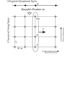
Figure 1: The original quantum spin ($\sigma$) chain and the ST-transformed two-dimensional Ising ($S$) system. The QTM $\cal T$ transfers along to the real direction.

2 QTM and the maximum eigenvalue

The Hamiltonian of the present transverse Ising quantum chain [23, 24] is defined as

$$-\beta{\cal H}=\sum_{i}^{N}\Big{(}K\sigma_{i}^{z}\sigma_{i+1}^{z}+\gamma\sigma_{i}^{x}\Big{)},\quad K=\beta J,\,\gamma=\beta\Gamma.$$ (6)

By the ST-transformation we have a two-dimensional Ising model shown in fig.1. Its partition function is [1, 2, 14]

$$Z_{m}=A_{m}^{Nm}{\rm Tr}\exp\Big{[}\sum_{i}^{N}\sum_{j}^{m}\frac{K}{m}S_{i,j}S_{i+1,j}+\gamma^{\prime}_{m}S_{i,j}S_{i,j+1}\Big{]}$$ (7)

where

$$\exp(-2\gamma^{\prime}_{m})=\tanh\frac{\gamma}{m},\qquad A_{m}=\Big{(}\frac{1}{2}\sinh\frac{2\gamma}{m}\Big{)}^{1/2}.$$ (8)

The system length $N$ is assumed to be infinite. The periodic boundary condition is required for the Trotter direction. We can see that the vertical (horizontal) interaction $\gamma_{m}^{\prime}$($\frac{K}{m}$) increases (decreases) as the temperature increases.

We apply the exact solution of the two-dimensional Ising model obtained by Schultz et. al.[25] using the transfer matrix method [26] to the present model. The QTM ${\cal T}$ is defined in a symmetric (and then hermitian) way as follows [2, 14].

$${\cal T}=V_{2}^{1/2}V_{1}V_{2}^{1/2}\quad\hbox{ with}$$

$$V_{1}=\Big{(}2\sinh\frac{2K}{m}\Big{)}^{m/2}\exp\big{(}K^{\prime}_{m}\sum_{j}^{m}S_{j}^{z}\big{)},\quad V_{2}=\exp(\gamma^{\prime}_{m}\sum_{j}^{m}S_{j}^{x}S_{j+1}^{x}),$$

$$\exp(-2K_{m}^{\prime})=\tanh\frac{K}{m}.$$ (9)

Here the spin operators $S^{x},S^{z}$ are used. The original quantum spin $\sigma^{z}_{i}$ is mapped to the Ising spin $S_{i,j}$ in eq.(7) and is remapped to $S^{x}$ in their formulation [25]. Then the correlation we want to evaluate is given by $\langle S_{0}S_{r}\rangle=\langle S_{0}^{x}S_{r}^{x}\rangle$ and it is a $z$-component correlation function of the original quantum chain as given in eq.(4).

The maximum eigenvalue $\lambda_{max}$ is given by[25]

$$\lambda_{max}=\Big{(}2\sinh\frac{2K}{m}\Big{)}^{m/2}\exp\big{(}{\frac{1}{2}\sum_{q}\varepsilon_{q}}\big{)},$$

$$\cosh\varepsilon_{q}=\coth\frac{2\gamma}{m}\coth\frac{2K}{m}-\hbox{cosec}\frac{2\gamma}{m}\hbox{cosec}\frac{2K}{m}\cos q,$$

$$q=\pm\frac{1}{m},\pm\frac{3}{m},\cdots,\pm\frac{m-1}{m},$$ (10)

with the help of Jordan-Wigner, Fourier transformation and Bogoliubov diagonalization. The associated maximum eigenvector is a vacuum of fermions.

We note that the critical line of the ST-transformed two-dimensional Ising model in eq.(7) is given by

$$1=\sinh\frac{2K}{m}\sinh 2\gamma_{m}^{\prime}=\sinh\frac{2K}{m}/\sinh\frac{2\gamma}{m}$$ (11)

as the ordinary two-dimensional Ising model. This means that our system is critical when $\gamma=K$ without the dependence of the Trotter number $m$ [27]. When $\gamma>K$ the system is disordered and when $\gamma<K$ it is ordered [24, 21].

3 Trotter-directional correlation functions

The correlation function $\langle S_{0}S_{r}\rangle_{m}$ at a finite temperature is expressed as an $r\times r$ Toeplitz determinant [25, 24, 23].

$$\langle S_{0}S_{r}\rangle_{m} =\langle\psi_{max}|S_{0}^{x}S_{r}^{x}|\psi_{max}\rangle_{m}$$ (17)

$$=\left|\begin{array}[]{lllll}g_{0}&g_{-1}&g_{-2}&&g_{1-r}\\ g_{1}&g_{0}&g_{-1}&\cdots&g_{2-r}\\ g_{2}&g_{1}&g_{0}&&g_{3-r}\\ &\vdots&&\ddots&\\ g_{r-1}&g_{r-2}&g_{r-3}&\cdots&g_{0}\\ \end{array}\right|$$

It becomes zz-correlation function of the original quantum Transverse Ising chain : $\langle\sigma^{z}(\tau)\sigma^{z}\rangle=\lim_{m\to\infty}\langle S_{0}S_{r}\rangle_{m}$. The matrix element $g_{k}$ is an expectation value of two fermions apart $k+1$ position and it is denoted as $a_{ij}$ in the reference [25].

$$g_{\pm k}=\frac{(-1)^{k}}{m}\sum_{q}e^{-ikq}\Big{[}\frac{1-e^{iq}e^{-2(\gamma+K)/m}}{1-e^{-iq}e^{-2(\gamma+K)/m}}\frac{1-e^{-iq}e^{2(\gamma-K)/m}}{1-e^{iq}e^{2(\gamma-K)/m}}\Big{]}^{1/2}$$

$$=\frac{(-1)^{k}}{m}\sum_{q>0}\frac{2\cosh(2K/m)\cos kq-e^{2\gamma/m}\cos(k+1)q-e^{-2\gamma/m}\cos(k-1)q}{\big{[}(\cosh(2\gamma/m)\cosh(2K/m)-\cos q)^{2}-(\sinh(2\gamma/m)\sinh(2K/m))^{2}\big{]}^{1/2}}$$

for $K>\gamma$. With the help of an integral formula

$$\frac{1}{\pi}\int_{0}^{\pi}\frac{1}{a+b\cos\theta}d\theta=\frac{1}{\sqrt{a^{2}-b^{2}}}\quad(a>b),$$ (19)

$g_{\pm k}$ becomes

$$g_{\pm k}=\frac{(-1)^{k}}{m\pi}\sum_{q>0}\int_{0}^{\pi}\frac{2\cosh(2K/m)\cos kq-e^{2\gamma/m}\cos(k+1)q-e^{-2\gamma/m}\cos(k-1)q}{\cosh(2\gamma/m)\cosh(2K/m)+\sinh(2\gamma/m)\sinh(2K/m)\cos\theta-\cos q}d\theta.$$ (20)

The integrand can be simplified by using formulae of trigonometric functions and $\sum_{q>0}\cos nq=0(n\neq 0)$. With the following $s$ and $s^{\prime}$ defined as

$$\cosh s=\cosh\frac{2\gamma}{m}\cosh\frac{2K}{m}+\sinh\frac{2\gamma}{m}\sinh\frac{2K}{m}\cos\theta,$$

$$s^{\prime}\sinh s=\sinh\frac{2\gamma}{m}\cosh\frac{2K}{m}+\cosh\frac{2\gamma}{m}\sinh\frac{2K}{m}\cos\theta,$$ (21)

the integrand becomes

$$m\sinh\frac{2\gamma}{m}\Big{(}s^{\prime}\sinh ks+\cosh ks\Big{)}+\sum_{q>0}\frac{2\sinh(2\gamma/m)}{\cos q-\cosh s}\sinh s\Big{(}s^{\prime}\cosh ks+\sinh ks\Big{)}$$

$$=m\frac{\sinh(2\gamma/m)}{\cosh(ms/2)}\Big{(}-s^{\prime}\sinh(\frac{m}{2}-k)s+\cosh(\frac{m}{2}-k)s\Big{)}.$$ (22)

Here we have used the following formula

$$\sum_{q>0}\frac{1}{\cos q-\cosh s}=-\frac{m}{2}\frac{\tanh(ms/2)}{\sinh s}.$$ (23)

Thus we have the matrix elements

$$g_{\pm k}=(-1)^{k-1}\frac{\sinh(2\gamma/m)}{\pi}\int_{0}^{\pi}\frac{1}{\cosh(ms/2)}\Big{[}s^{\prime}\sinh(\frac{m}{2}-k)s\mp\cosh(\frac{m}{2}-k)s\Big{]}\ d\theta,(k\geq 1)$$

$$g_{0}=\cosh\frac{2\gamma}{m}-\frac{\sinh(2\gamma/m)}{\pi}\int_{0}^{\pi}s^{\prime}\tanh\frac{ms}{2}\ \ d\theta.$$ (24)

These are valid for the both cases of $\gamma\geq K$ and $\gamma\leq K$. We note here that $g_{k}$ satisfies

$$g_{k}(\gamma)=g_{-k}(-\gamma),\qquad g_{m-k}(\gamma)=(-1)^{m-1}g_{-k}(\gamma)\quad(k\neq 0).$$ (25)

We can easily check that $\langle S_{0}S_{m}\rangle_{m}=\langle S_{0}S_{0}\rangle_{m}=1$ is fulfilled.

The magnetization $\langle\sigma^{x}\rangle$ of the original quantum spin chain is related to the nearest neighbor correlation function $\langle S_{0}S_{1}\rangle_{m}=g_{0}$ as follows [14].

$$\langle\sigma^{x}\rangle=\lim_{m\to\infty}\coth\frac{2\gamma}{m}-g_{0}/\sinh\frac{2\gamma}{m}=\lim_{m\to\infty}\frac{1}{\pi}\int_{0}^{\pi}s^{\prime}\tanh\frac{ms}{2}\ d\theta.$$ (26)

For large $m$, $s$ and $s^{\prime}$ in eq.(3) becomes

$$s\simeq\frac{2}{m}\sqrt{\gamma^{2}+K^{2}+2\gamma K\cos\theta},\qquad s^{\prime}\simeq\frac{\gamma+K\cos\theta}{\sqrt{\gamma^{2}+K^{2}+2\gamma K\cos\theta}},$$ (27)

and thus we reproduce the exact solution.

The diagonal correlation function is expressed as a four-body Ising spins correlation as follows. Using a Ising spin state $|S\rangle$ and its completeness $\sum_{\{S\}}|S\rangle\langle S|=1$, we obtain

$$\langle\sigma^{x}(\tau)\sigma^{x}\rangle =\lim_{m\to\infty}\sum_{\{S,S^{\prime},S^{\prime\prime},S^{\prime\prime\prime}\}}\langle S|e^{-\beta{\cal H}}e^{\tau{\cal H}}|S^{\prime}\rangle\langle S^{\prime}|e^{2\gamma_{m}^{\prime}S^{\prime}S^{\prime\prime}}|S^{\prime\prime}\rangle\langle S^{\prime\prime}|e^{\tau{\cal H}}|S^{\prime\prime\prime}\rangle\langle S^{\prime\prime\prime}|e^{2\gamma_{m}^{\prime}S^{\prime}S^{\prime\prime}}|S\rangle/Z_{m}$$ (28)

$$=\lim_{m\to\infty}\frac{1}{\sinh^{2}(2\gamma/m)}\Big{\langle}\big{(}\cosh\frac{2\gamma}{m}-S_{r+1}S_{r}\big{)}\big{(}\cosh\frac{2\gamma}{m}-S_{1}S_{0}\big{)}\Big{\rangle}_{m}.$$

Here we have used an identity,

$$\langle S|\sigma^{x}e^{\gamma\sigma^{x}/m}|S^{\prime}\rangle=e^{-2\gamma_{m}^{\prime}SS^{\prime}}\langle S|e^{\gamma\sigma^{x}/m}|S^{\prime}\rangle.$$ (29)

The 4-body correlation of Ising spins on the same Trotter axis is expressed by $g_{k}$ as

$$\langle S_{0}S_{1}S_{r}S_{r+1}\rangle_{m}=g_{0}^{2}-g_{r}g_{-r}.$$ (30)

Thus we have

$$\langle\sigma^{x}(\tau)\sigma^{x}\rangle =\lim_{m\to\infty}\frac{1}{\sinh^{2}(2\gamma/m)}\Big{(}\cosh^{2}\frac{2\gamma}{m}-2g_{0}^{2}\cosh\frac{2\gamma}{m}+(g_{0}^{2}-g_{r}g_{-r})\Big{)}$$ (31)

$$=\langle\sigma^{x}\rangle^{2}-\lim_{m\to\infty}\frac{1}{\sinh^{2}(2\gamma/m)}g_{r}g_{-r}.$$

Similarly, the $yy$-correlation function is given by

$$\langle\sigma^{y}(\tau)\sigma^{y}\rangle =\lim_{m\to\infty}\frac{1}{\sinh^{2}(2\gamma/m)}\Big{\langle}(-iS_{r})\big{(}\cosh\frac{2\gamma}{m}-S_{r+1}S_{r}\big{)}(-iS_{0})\big{(}\cosh\frac{2\gamma}{m}-S_{1}S_{0}\big{)}\Big{\rangle}_{m}$$

$$=\lim_{m\to\infty}\frac{-1}{\sinh^{2}(2\gamma/m)}\Big{[}(\cosh^{2}\frac{2\gamma}{m}+1)\langle S_{0}S_{r}\rangle_{m}-\cosh\frac{2\gamma}{m}\big{(}\langle S_{0}S_{r+1}\rangle_{m}+\langle S_{1}S_{r}\rangle_{m}\big{)}\Big{]}$$

and which satisfies the following identity [28] for the present model at the limit $m\to\infty$.

$$\frac{d^{2}}{d\tau^{2}}\langle\sigma^{z}(\tau)\sigma^{z}\rangle=\Gamma^{2}\langle\sigma^{y}(\tau)\sigma^{y}\rangle.$$ (33)

4 Evaluation of the $\left\langle S_{0}S_{r}\right\rangle_{m}$ correlation functions

We study the $r$ and the temperature dependencies of the correlation functions $\langle S_{0}S_{r}\rangle_{m}$ in this section. We cannot apply Szegö’s theorem [29] to our Toeplitz determinant in eq.(17). If we take $m\to\infty$ for a fixed $r$, all $g_{k}$ becomes $0$ except $g_{0}\to 1$ and thus we always have a wrong result $\langle S_{0}S_{r}\rangle_{m}=1$. We need to evaluate the determinant with a finite $m$ and then take $m\to\infty$ limit at final to get a correct result of the original quantum chain [2].

Define $\delta=r/m$ to indicate the normalized distance of two spins. We assume $m$ and $r$ are very large but finite. We take a perturbative approach for the small $\delta$ in the first subsection. We do numerical computation for the general $\delta$ in the successive subsections.

4.1 Analytic approach for the small $\delta$

We calculate the determinant for the small $\delta$ up to the second order analytically. Expand the matrix elements $g_{k}$ up to $k^{2}$ order,

$$g_{\pm k}\simeq(-1)^{k}\sinh\frac{2\gamma}{m}\Big{[}\pm 1-\frac{1}{\pi}\int_{0}^{\pi}s^{\prime}\tanh\frac{ms}{2}\ d\theta$$

$$\qquad+k\frac{1}{\pi}\int_{0}^{\pi}s(s^{\prime}\mp\tanh\frac{ms}{2})\ d\theta+\frac{k^{2}}{2}\frac{1}{\pi}\int_{0}^{\pi}s^{2}(\pm 1-s^{\prime}\tanh\frac{ms}{2}\ d\theta\Big{]}.$$ (34)

In general the determinant of a Toeplitz matrix whose elements has up to $k^{2}$ dependence can be obtained with the help of the standard matrix procedure and is given in Appendix A.

After tedious but straightforward calculation we have

$$\langle S_{0}S_{r}\rangle_{m} =1+c_{1}(m)\delta+c_{2}(m)\delta^{2}+O(\delta^{3})$$

with $$c_{1}(m)=-2\gamma I_{0}-\frac{4\gamma}{3m^{2}}\big{(}2\gamma^{2}I_{0}-2\gamma I_{1}+I_{3}\big{)}+O(m^{-4}),$$ (35)

$$c_{2}(m)=2\gamma^{2}-\frac{4\gamma^{2}}{3m^{2}}\big{(}I_{1}^{2}-I_{0}I_{2}+K^{2}\big{)}+O(m^{-4}).$$

Where integrals are defined as

$$I_{0}=\frac{1}{\pi}\int_{0}^{\pi}\frac{\gamma+K\cos\theta}{\sqrt{\gamma^{2}+K^{2}+2\gamma K\cos\theta}}\tanh\sqrt{\gamma^{2}+K^{2}+2\gamma K\cos\theta}\ d\theta=\langle\sigma^{x}\rangle,$$

$$I_{1}=\frac{1}{\pi}\int_{0}^{\pi}\sqrt{\gamma^{2}+K^{2}+2\gamma K\cos\theta}\tanh\sqrt{\gamma^{2}+K^{2}+2\gamma K\cos\theta}\ d\theta,$$

$$I_{2}=\frac{1}{\pi}\int_{0}^{\pi}(\gamma+K\cos\theta)\sqrt{\gamma^{2}+K^{2}+2\gamma K\cos\theta}\tanh\sqrt{\gamma^{2}+K^{2}+2\gamma K\cos\theta}\ d\theta,$$

$$I_{3}=\frac{1}{\pi}\int_{0}^{\pi}\Big{(}\frac{\gamma K^{2}(\gamma^{2}+2K^{2}+3\gamma K\cos\theta)\sin^{2}\theta}{\sqrt{\gamma^{2}+K^{2}+2\gamma K\cos\theta}^{3}}\tanh\sqrt{\gamma^{2}+K^{2}+2\gamma K\cos\theta}$$

$$\qquad\qquad\qquad+\frac{\gamma^{2}K^{2}(\gamma+K\cos\theta)\sin^{2}\theta}{(\gamma^{2}+K^{2}+2\gamma K\cos\theta)\cosh^{2}\sqrt{\gamma^{2}+K^{2}+2\gamma K\cos\theta}}\Big{)}\ d\theta.$$ (36)

The first integral $I_{0}$ is nothing but the magnetization $\langle\sigma^{x}\rangle=-\frac{\partial}{\partial\gamma}(\beta f)$ of the original quantum chain. It takes a finite value between 0 and 1 depending on the ratio $K/\gamma$ in the low temperature region and it becomes $\gamma$ at the high temperature limit.

We can check easily that the result eq.(4.1) agrees with a perturbative calculation of the temperature Green function for a small $\tau=\beta\delta$ ,

$$\langle\sigma^{z}(\tau)\sigma^{z}\rangle=\Big{\langle}\big{(}\sigma^{z}+[{\cal H},\sigma^{z}]\tau+\frac{1}{2}[{\cal H},[{\cal H},\sigma^{z}]]\tau^{2}+\cdots\big{)}\sigma^{z}\Big{\rangle}=1-2\Gamma\langle\sigma^{x}\rangle\tau+2\Gamma^{2}\tau^{2}+\cdots.$$ (37)

4.2 Numeric evaluation for $K/\gamma=0.7$ in the disordered region.

To study the behavior of our correlation functions for the whole range of the parameters $\delta$ and the temperature we perform a direct numerical computation of the integrals of eq.(3) and the determinant of eq.(17). The data are taken for $K/\gamma=0.7,1.0,1.3,2.0$, $m=8\sim 1024$ and $\gamma=0.1\sim 64$ while $\gamma/m<1$. The distance $r$ varies $r=1,2,3,\cdots,m/2,m/2+1$. Due to the periodicity for the Trotter direction, our correlation function has the same value at $r$ and at $m-r$. It is a good test for our numeric computation whether the function has the same value at $r=m/2-1$ and $r=m/2+1$ or not. Our data has 9 digits accuracy even in the worst case.

Figure 2 is the $\delta$ dependence of the correlation function for the high temperature $K=0.7$ and $\gamma=1$. We omit the data for $\delta>1/2$. It takes the lowest value at $\delta=1/2$. Its $m$-dependence is very week as was shown in the analytic evaluation in eq.(4.1) ($m^{-2}$ dependence) so that we can not distinguish each curves of the different $m$ in this figure.

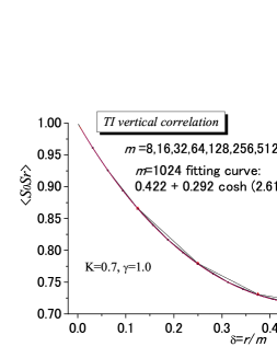
Figure 2: $\langle S_{0}S_{r}\rangle_{m}$ versus $\delta=r/m$ at $K=0.7$ and $\gamma=1.0$ for various $m=8\sim 1024$. The fitting curve for $m=1024$ is also drawn.

We adopt the following two parameters ($b$ and $c$) fitting curve to analyze the $\delta$ dependence,

$$f_{H}(\delta)=1-\Big{(}\cosh(c/2)-\cosh(c(1/2-\delta))\Big{)}/\cosh b$$ (38)

which satisfies $f_{H}(0)=1$. This curve is exact for $K=0$ as shown in Appendix B.

$$\langle S_{0}S_{r}\rangle_{m}=\cosh(\gamma(1-2\delta))/\cosh\gamma.\qquad(c=2\gamma,\,\,b=\gamma)$$ (39)

The fitting gives excellently good agreement to the numerical data as shown in fig.2.

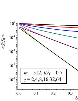
Figure 3: Semi-log plot of correlation functions versus $\delta$ for $\gamma=2,4,8,16,32,64$ from top to bottom. $K/\gamma=0.7$ and $m=512$. Two thin lines are fitting curves of eq.(4.2).

At a low temperature the correlation function shows exponential decay as shown in fig.3. We use a new fitting curve which does not satisfy $f_{L}(0)=1$ any more to estimate the main term.

$$f_{L}(\delta)=\cosh(c(1/2-\delta))/\cosh b.$$ (40)

The results are

$$\cosh(21.2(1/2-\delta))/\cosh 11.8\quad\hbox{ for }\quad\gamma=32,$$

$$\cosh(40.6(1/2-\delta))/\cosh 21.8\quad\hbox{ for }\quad\gamma=64,$$ (41)

and are drawn in fig. 3. The values of $b$ and $c$ for $\gamma=64$ are about twice larger than those for $\gamma=32$, respectively.

To study the temperature dependence we plot the data for $\delta=1/2$ in fig.4. The exponential decay for the $\gamma$ is clearly shown. By fitting the exponential function to the data of $m=32,128,512$, we estimate the gradient approximately

$$\exp(-0.32\gamma).$$ (42)

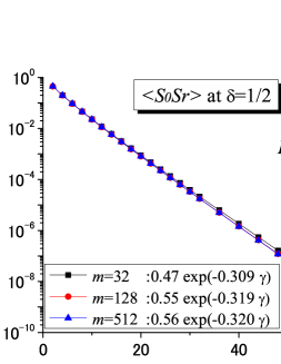
Figure 4: Semi-log plot of the correlation function at $\delta=1/2$ versus $\gamma$. $K/\gamma=0.7$. $m=32,128,512$. Lines are fitting curves shown in the legend.

From these results we conclude that the correlation function decays exponentially to zero for both the $\delta$ and the temperature ($\gamma$) in the disordered region.

4.3 Critical region: $K=\gamma$

We show two graphs figs. 5 and 6 for $m=1024$. The former shows the $\delta$-dependence and the latter shows the $\gamma$-dependence. The both graphs clearly show a power law behavior of the correlation functions in the low temperature. The fitting line for $\gamma=64$ in fig.5 is

$$1.01\times r^{-0.24}.$$ (43)

The fitting line shown in fig.6 for $r=512$ ($\delta=1/2$) is

$$0.72\times\gamma^{-0.25}.$$ (44)

These exponents remind us the two-dimensional Ising model which has $\eta=1/4$ and $\beta=1/8$.

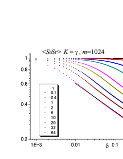
Figure 5: Log-log plot versus $\delta$ for various $\gamma$. $K=\gamma$ and $m=1024$. The line for $\gamma=64$ is a fitting curve given in eq.(43).

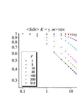
Figure 6: Log-log plot versus $\gamma$ for various position $r$. The line is a fitting curve for $r=512$ given in eq.(44).

4.4 Ordered region: $K/\gamma=1.3$

The big difference from the other regions is that the correlation function decreases and saturates to some value as the temperature decreases in the ordered region. In fig.7 the saturated value is about 0.8 for $K/\gamma=1.3$. This means the quantum fluctuation is small in this region. The increase for the large $\delta$ and the low temperature ($\gamma>2$) is due to the finite $m$. As is seen in fig.8, this increase disappears as $m\to\infty$.

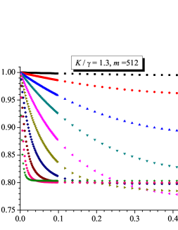
Figure 7: Normal plot of $m=512$ for the several temperatures.

We estimate the saturation values as follows. Plot the data of $\delta=1/2$ versus $1/m$ in fig.8. Fit them with a quadratic equation of $1/m$ and find the limit values of $m\to\infty$ for each temperature. Three these fitting curves are also drawn in fig.8. The three limit values almost coincide to each others such that $0.79934$ for $\gamma=32$, $0.79928$ for $\gamma=48$ and $0.79912$ for $\gamma=64$. Thus we conclude the saturation value for $K/\gamma=1.3$ at the zero temperature is about 0.799.

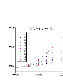
Figure 8: Saturation values versus $m^{-1}$ for $K/\gamma=1.3$. $\gamma=64\sim 32$ from top to bottom. $m=224,256,320,384,448,512,640,768,896,1024$. Fitting curves are quadratic equations of $1/m$.

Additionally, when $K/\gamma=2.0$ the saturation value is estimated about 0.930.

These values are equal to the square of the order parameter $\langle\sigma^{z}\rangle^{2}=(1-\gamma/K)^{1/4}$ at $T=0$ [24, 22, 21].

When $\gamma=0$ ($K/\gamma=\infty$), the value is $\langle S_{0}S_{r}\rangle_{m}=1$ for any $r$ since $g_{\pm k}=0$ and $g_{0}=1$.

5 Auto correlation functions

We assume that the analytic continuation from the temperature Green function to the time-dependent auto-correlation function is achieved by just replacing $\tau$ with the imaginary time $it$ in the present case. This assumption is confirmed by deriving the same result as the known results [20, 22, 19, 16, 18, 21].

5.1 $\langle\sigma^{z}(t)\sigma^{z}\rangle$

When $t\simeq 0$, replacing $\delta\to\tau/\beta\to it/\beta$ in eq.(4.1) for $m=\infty$,

$$\langle\sigma^{z}(t)\sigma^{z}\rangle=\lim_{m\to\infty}\langle S_{0}S_{r}\rangle_{m}=1-2i\Gamma\langle\sigma^{x}\rangle t-2\Gamma^{2}t^{2}+O(t^{3})$$ (45)

This result agrees to Brandt and Jacoby[18] and Perk et.al.[19] with rescaling $t$ by $t/2$ due to the definition of the Hamiltonian.

We adopt the following functions for the general $t$ with many fitting parameters to fit whole the range $0\leq\delta\leq 1/2$ of the numerical data shown in figs.3,5 and 7. Each fitting function is chosen to have the main exponential or power decay terms found in §4. $\delta$ is replaced to $\tau=\beta\delta$ ($\beta=\gamma$). The used data are for $m=512$ and $\gamma=10$. The results are

$$0.028+0.48e^{-2.7\tau}+0.64e^{-0.74\tau}+\frac{3.1e^{-0.44\tau}}{\tau-20.}\qquad\hbox{for }\gamma=10,K=7,$$ (46)

$$-2.9+8.3(1-1.0e^{0.041\tau})\tau^{-1/4}+0.30e^{-2.7\tau}+3.7e^{0.048\tau}\qquad\hbox{for }\gamma=K=10,$$ (47)

$$0.85+\frac{0.088e^{-2.2\tau}}{0.44+\tau}-\frac{270e^{0.032\tau}}{(70+\tau)^{2}}+\frac{4700e^{-2.5\tau}}{(400+\tau)^{3}}\qquad\hbox{for }\gamma=10,K=13$$ (48)

and are shown in figs.9 after replacing $\tau$ to $it$.

Figure 9: Time dependence of the auto-correlation functions $\langle\sigma^{z}(t)\sigma^{z}\rangle$. Solid lines are real part and dotted lines are imaginary part of the functions. The graph of $\gamma=10,K=7$ should be compared to figs. 3 and 4 of Perk and Au-Yang [22], and the graph of $\gamma=10,K=13$ to figs. 6 and 7 of it.

These shows almost the same characteristic behavior obtained by many authors [22, 18, 20, 21] such that a fast+slow oscillating decay around zero for $\gamma>K$, a simple oscillating decay for $\gamma=K$ and a saturation to a non-zero value with a oscillation for $\gamma<K$. It is, as is well known, not easy to get accurate results by an analytic continuation from numerical data. We need to consider $m$ dependence to get more accurate result as has done in §4 or need a more sophisticated method. It is instructive that the Trotter number $m=512$ is large enough to estimate the leading singularity as shown in §4, however, it is small to estimate the whole range of the time dependence of the auto-correlations quantitatively. The present result is an example obtained by a simple extrapolation.

5.2 $\langle\sigma^{x}(t)\sigma^{x}\rangle$

Substitute $g_{r}$ and $\tau=it=\beta r/m$ into eq.(31) and take the limit $m\to\infty$ we have

$$\langle\sigma^{x}(t)\sigma^{x}\rangle=\langle\sigma^{x}\rangle^{2}-\bigg{[}\frac{1}{\pi}\int_{0}^{\pi}\frac{\Gamma+J\cos\theta}{w}\Big{(}\tanh\beta w\cosh(2iwt)-\sinh(2iwt)\Big{)}d\theta\bigg{]}^{2}$$

$$\qquad\qquad\qquad+\bigg{[}\frac{1}{\pi}\int_{0}^{\pi}\Big{(}\cosh(2iwt)-\tanh\beta w\sinh(2iwt)\Big{)}d\theta\bigg{]}^{2}$$ (49)

for a finite temperature where we have abbreviated $w=\sqrt{\Gamma^{2}+J^{2}+2\Gamma J\cos\theta}$. Thus we have obtained the Niemeijer’s exact result [16, 17, 20] by extending the QTM method.

6 Summary and Discussions

We have studied the Trotter-directional correlation function which is interpreted as a Matsubara’s temperature Green function by the Quantum Transfer Matrix method.

By applying analytic continuation to the correlation function we examined the auto-correlation functions $\langle\sigma^{z}(t)\sigma^{z}\rangle$ and $\langle\sigma^{x}(t)\sigma^{x}\rangle$. The numerical result for the $zz$-correlation caught the characteristic behavior of the time dependence of them. We have re-derived the $xx$-correlation exactly.

Our formulation are based on the ST-transformation and thus $\beta/m$ should be small enough to get a meaningful result of the relevant quantum systems. In practice we use a discrete $\tau=\beta\delta=\beta r/m$ to estimate the continuous $\tau$ or $t$ dependence of auto-correlations. Thus we need a large $m$ to get more accurate results in numerical calculation.

We have demonstrated that the Trotter-directional correlation function is a useful tool to measure the quantum fluctuations. It has the same value of the square of the order parameter $\langle\sigma^{z}\rangle^{2}$ at $T=0$. The shrinkage of a spin length which is given as the order parameter is often used as a measure of the quantum fluctuation. While the order parameter $\langle\sigma^{z}\rangle$ is zero for $T>0$ for the present one-dimensional system and then it can not be used as a measure, our correlation has a finite value which varies from $\langle\sigma^{z}\rangle^{2}(T=0)$ to 1 ($T=\infty$). When $\gamma=0$ which means no quantumness (1 dimensional classical Ising model) , our correlation is equal to one and thus indicates no quantum fluctuation correctly. The square of the magnetization $\langle\sigma^{z}\rangle^{2}\simeq\langle\sigma_{0}\sigma_{R}\rangle$ ($R\to\infty$) is considered as a projection to an another spin in distance $R$. Our correlation $\langle\sigma_{i}^{z}(\tau)\sigma_{i}^{z}\rangle$ is a projection of itself and also it shows how the fluctuation increases as a function of ”time”($\tau$). Thus our correlation function and the order parameter are complemental measures for the quantum fluctuation.

We emphasize that the Trotter-directional correlation function can be defined for any ST-transformed classical systems mapped from quantum systems. What we should observe is the classical Ising spins $\{S\}$ and thus we can easily done by the Quantum Monte Carlo simulation or others. By using many Ising spins which are on different stacked layers or different real positions, we can study general many temperature/time Green functions.

Finally we mention Bethe-Ansatz systems. The maximum eigenvalue and the associated eigenvector of the Heisenberg chain are well known [3, 6, 10] so that the application our method to them is a future problem.

Appendix A: Determinant of a Toeplitz Matrix

The determinant of the $r\times r$ Toeplitz matrix with the elements

$$M_{i,j}=\left\{\begin{array}[]{cc}a+(i-j)b+(i-j)^{2}c&:1\leq j<i\leq r\\ X_{0}&:1\leq i=j\leq r\\ d+(j-i)e+(j-i)^{2}f&:1\leq i<j\leq r\\ \end{array}\right.$$ (50)

is expressed as follows.

$$\hbox{det}M= \Big{(}\frac{c}{c-f}\Big{)}^{3}(A_{0})^{r}-\Big{(}\frac{f}{c-f}\Big{)}^{3}(\overline{A_{0}})^{r}$$ (51)

$$-\frac{(A_{0})^{r-1}}{(c-f)^{3}}\bigg{[}\Big{\{}-6c^{2}fA_{0}p(r+1)-\overline{z_{3}}p(r)+\overline{z_{2}}p(r-1)\Big{\}}/2$$

$$\qquad\qquad-rc\Big{\{}(\overline{z_{1}}+4cf(c-f))p(r)-\overline{z_{1}}p(r-1)\Big{\}}$$

$$\qquad\qquad+r^{2}c^{2}f(c-f)\Big{\{}p(r)-p(r-1)\Big{\}}\bigg{]}$$

$$-\frac{(A_{0})^{r-2}}{(c-f)^{3}}\bigg{[}\Big{\{}6cf^{2}A_{0}^{2}q(r+1)+A_{0}z_{3}q(r)-\overline{A_{0}}z_{2}q(r-1)\Big{\}}/2$$

$$\qquad\qquad+rf\Big{\{}A_{0}(z_{1}-4cf(c-f))q(r)-\overline{A_{0}}z_{1}q(r-1)\Big{\}}$$

$$\qquad\qquad+r^{2}cf^{2}(c-f)\Big{\{}A_{0}q(r)-\overline{A_{0}}q(r-1)\Big{\}}\bigg{]}.$$

Here

$$z_{1}=c^{2}e-f^{2}b+2bcf+2cf(c-f),$$

$$z_{2}=c^{2}e^{2}+2c(-cd+(b+c)e)f+(b^{2}+4bc+2c(2a-3X_{0}+c+3d))f^{2}-2(a+b+c)f^{3},$$

$$z_{3}=z_{2}-4fz_{1}+2cf^{2}(3a-3X_{0}+3b+3e+c-f),$$

$$A_{0}=X_{0}-d,\qquad A_{1}=-3X_{0}+a+b+c+2d+e-f.$$ (52)

The symbol overline $\overline{z}$ means an exchange $(a,b,c)\leftrightarrow(d,e,f)$ of $z$. (transpose of the matrix) And

$$p(k) =\frac{1}{(\alpha-\beta)(\beta-\gamma)(\gamma-\alpha)}\Big{[}\alpha^{k+1}(\beta-\gamma)+\beta^{k+1}(\gamma-\alpha)+\gamma^{k+1}(\alpha-\beta)\Big{]},$$ (53)

$$q(k) =\frac{1}{(\alpha-\beta)(\beta-\gamma)(\gamma-\alpha)}\Big{[}(\alpha\beta)^{k}(\alpha-\beta)+(\beta\gamma)^{k}(\beta-\gamma)+(\alpha\gamma)^{k}(\gamma-\alpha)\Big{]},$$

$$\overline{p(k)}=\Big{(}A_{0}/\overline{A_{0}}\Big{)}^{k-1}q(k).$$

$\alpha,\beta,\gamma$ are roots of $A_{0}x^{3}+A_{1}x^{2}-\overline{A_{1}}x-\overline{A_{0}}=0$ .

Multiply $(-1)^{i}\times(-1)^{j-1}=(-1)^{i-j-1}$ to $M_{i,j}$ to suite our matrix $M^{\prime}$ with elements:

$$M^{\prime}_{i,j}=\left\{\begin{array}[]{cc}(-1)^{i-j-1}\big{\{}a+(i-j)b+(i-j)^{2}c\big{\}}&:1\leq j<i\leq r\\ -X_{0}&:1\leq i=j\leq r\\ (-1)^{j-i-1}\big{\{}d+(j-i)e+(j-i)^{2}f\big{\}}&:1\leq i<j\leq r\\ \end{array}\right..$$ (54)

The relation $M$ and $M^{\prime}$ is

$$\hbox{det}M^{\prime}=(-1)^{r}\hbox{det}M.$$ (55)

Appendix B: $\langle S_{0}S_{r}\rangle_{m}$ for $K=0$ (derivation of Eq.(39))

When $K=0$, the system reduces to a one-dimensional Ising chain for the Trotter direction with a spin interaction $\gamma^{\prime}_{m}$. The correlation function is simply given by

$$\langle S_{0}S_{r}\rangle_{m}=\frac{\tanh^{r}\gamma^{\prime}_{m}+\tanh^{m-r}\gamma^{\prime}_{m}}{1+\tanh^{m}\gamma^{\prime}_{m}}=\frac{\cosh(\gamma(1-2\delta))}{\cosh\gamma}$$ (56)

under the periodic boundary condition with using eq.(2).

Alternatively, we can derive this result from eq.(17). The $s$ and $s^{\prime}$ of eq.(3) are now

$$s=\frac{2\gamma}{m},\quad s^{\prime}=1.$$ (57)

The elements $g_{k}$ are simplified as

$$g_{\pm k}=(-1)^{k-1}\frac{\sinh(2\gamma/m)}{\cosh\gamma}\Big{[}\mp\exp\big{(}\mp(1-\frac{2k}{m})\big{)}\gamma\Big{]},$$

$$g_{0}=\cosh\frac{2\gamma}{m}-\sinh\frac{2\gamma}{m}\tanh\gamma.$$ (58)

Thus the matrix of eq.(17) can be diagonalized and the determinant is obtained directly.

As the third method, we can derive the result eq.(56) without the ST-transformation by using a Heisenberq equation:

$$\frac{d}{d\tau}\sigma^{z}(\tau)=[{\cal H},\sigma^{z}(\tau)],\qquad\sigma^{z}(\tau)=e^{{\cal H}\tau}\sigma^{z}e^{-{\cal H}\tau}$$ (59)

where $\tau$ is imaginary time and ${\cal H}=-\sum_{j}\Gamma\sigma_{j}^{x}$. Using twice this equation, $\sigma^{z}(\tau)$ follows a differential equation and it becomes as

$$\frac{d^{2}}{d\tau^{2}}\sigma^{z}(\tau)=\Gamma^{2}\sigma^{z}(\tau),\qquad\sigma^{z}(\tau)=c_{1}e^{2\Gamma\tau}+c_{2}e^{-2\Gamma\tau}.$$ (60)

$c_{1}$ and $c_{2}$ are constant $2\times 2$ matrices and are defined by an initial $\langle\sigma^{z}(0)\sigma^{z}\rangle=1$ and a periodicity $\langle\sigma^{z}(\tau)\sigma^{z}\rangle=\langle\sigma^{z}(\beta-\tau)\sigma^{z}\rangle$ conditions[15]. We have again

$$\langle\sigma^{z}(\tau)\sigma^{z}\rangle=\lim_{m\to\infty}\langle S_{0}S_{r}\rangle_{m}=\frac{\cosh(\gamma-2\Gamma\tau))}{\cosh\gamma}.\quad(\Gamma\tau=\gamma\delta).$$ (61)

References

[1]
M. Suzuki: Phys. Rev. B31 (1985) 2957.
[2]
M.Suzuki, and M. Inoue: Prog. Theor. Phys. 78 (1987) 787;
M.Inoue, and M. Suzuki: Prog. Theor. Phys. 79 (1988) 645.
[3]
T. Koma: Prog.Theor. Phys. 78 (1987) 1213.
[4]
M. Takahashi: Phys. Rev. B43 (1991) 5788.
[5]
C. Destri, and H.J. de Vega: Phys. Rev. Lett. 69 (1992) 2313;
C. Destri, and H.J. de Vega: Nucl. Phys. B504 (1997) 621.
[6]
A. Klümper: Ann. Physik 1 (1992) 540;
A. Klümper: Z. Phys. B91 (1993) 507;
A. Klümper: Eur. Phys. J. B5 (1998) 677.
[7]
J. Suzuki, Y. Akutsu, and M. Wadachi: J. Phys. Soc. Jpn. 59 (1990) 2667;
J. Suzuki, T. Nagao, and M. Wadachi: Int. J. Mod. Phys. B6 (1992) 1119;
H. Mizuta, T. Nagao, and M. Wadachi: J. Phys. Soc. Jpn. 63 (1994) 3951.
[8]
J. Jüttner, A. Klümper, and J. Suzuki: Nucl. Phys. B487 (1997) 335.
[9]
K. Sakai, M. Shiroishi, J. Suzuki, and Y. Umeno: Phys. Rev. B60 (1999) 5186.
[10]
F. Göhmann, A. Klümper, and A. Seel: J.Phys. A37 (2004) 7625.
[11]Quantum Monte Carlo Method in Condensed Matter Physics, ed. M. Suzuki, (World Scientific,1993);
Quantum Monte Carlo Methods in Equilibrium and Non-equilibrium Systems,
ed. M. Suzuki, (Springer, SSS74, 1987).
[12]
M. Suzuki: Prog. Theor. Phys. 56 (1976) 183.
[13]
H. De Raedt, and B. De Raedt: Phys. Rep. 127 (1983) 233.
[14]
M. Suzuki: J. Stat. Phys. 110 (2003) 945;
A. Sugiyama, H. Suzuki, and M. Suzuki: Physica A368 (2006) 449.
[15]
A.A. Abrikosov, L.P.Gorkov and I.E. Dzyaloshinski:
Methods of Quantum Field Theory in Statistical Physics ,
(Dover Publications, 1975)
[20]
G. Müller and R.E.Shrock: Phys. Rev. B29 (1984) 288.
[21]
S. Sachdev and A.P. Young: Phys. Rev. Lett. 78 (1997) 2220;
S. Sachdev: Quantum Phase Transitions, (Cambridge, 1999).
[22]
J.H.H. Perk and H. Au-Yang: J. Stat.Phys. 135 (2009) 599;
[23]
E.H. Lieb, T. D.Schultz, and D.C. Mattis: Ann. Phys. 16 (1961) 407;
S. Katsura: Phys. Rev. 127 (1962) 1508;
E. Barouch, and B. M. McCoy: Phys. Rev. A3 (1971) 786.
[24]
P. Pfeuty: Ann. Phys. 57 (1970) 79.
[25]
T.D. Schultz, D.C. Mattis, and E.H. Lieb: Rev. Mod. Phys.36 (1964) 856.
[26]
R. Kubo: Busseiron Kenkyu 1 (1943) 1 [in Japanese];
H.A.Kramers, and G.H. Wannier: Phys. Rev. 60 (1941) 252.
[27]
M. Inoue, and M. Suzuki: Prog. Theor. Phys. 79 (1988) 30.
[28]
J. Lajzerowicz and P. Pfeuty: Phys. Rev. B 11 (1975) 4560.
[29]
B.M.McCoy and T.T.Wu: The Two-dimensional Ising Model,
(1973) Harvard univ. press.