Field-induced decay of quantum vacuum: visualizing pair production in a classical photonic system

Abstract

The phenomenon of vacuum decay, i.e. electron-positron pair production due to the instability of the quantum electrodynamics vacuum in an external field, is a remarkable prediction of Dirac theory whose experimental observation is still lacking. Here a classic wave optics analogue of vacuum decay, based on light propagation in curved waveguide superlattices, is proposed. Our photonic analogue enables a simple and experimentally-accessible visualization in space of the process of pair production as break up of an initially negative-energy Gaussian wave packet, representing an electron in the Dirac sea, under the influence of an oscillating electric field.

I Introduction

Quantum-classical analogies have been exploited on many occasions to mimic at a macroscopic level many quantum phenomena which are currently inaccessible in microscopic quantum systems Dragomanbook . In particular, in the past decade engineered photonic structures have provided a useful laboratory tool to investigate and visualize with classical optics the dynamical aspects embodied in a wide variety of coherent quantum phenomena encountered in atomic, molecular, condensed-matter and matter-wave physics Longhi09LPR . Among others, we mention the optical analogues of electronic Bloch oscillations B01 ; B02 and Zener tunneling ZT ; Dreisow09 , dynamic localization DL , coherent enhancement and destruction of tunneling CDT , adiabatic stabilization of atoms in ultrastrong laser fields stabi , Anderson localization AL , quantum Zeno effect QZ , coherent population transfer STIRAP , and coherent vibrational dynamics molecule . Most of the above mentioned studies are based on the formal analogy between paraxial wave equation of optics in dielectric media and the single-particle nonrelativistic Schrödinger equation, thus providing a test bed for classical analogue studies of nonrelativistic quantum phenomena. Recently, a great attention has been devoted toward the investigation of experimentally-accessible and controllable classical or quantum systems that simulate certain fundamental phenomena rooted in the relativistic Dirac equation. Among others, cold trapped atoms, ions and graphene have proven to provide accessible systems to simulate relativistic physics in the lab, and a vast literature on this subject has appeared in the past few years (see, for instance, GR1 ; GR2 ; ion and references therein). In particular, low-energy excitations of nonrelativistic two-dimensional electrons in graphene obey the Dirac-Weyl equation and behave like massless relativistic particles. This has lead to the predictions in condensed-matter physics of phenomena analogous to Zitterbewegung Zitterbewegung and Klein tunneling Klein of relativistic massive or massless particles, with the first experimental evidences of Klein tunneling in graphene EGR1 and in carbon nanotube EGR2 systems. Photonic analogues of Dirac-type equations have been also theoretically proposed for light propagation in certain triangular or honeycomb photonic crystals, which mimic conical singularity of energy bands of graphene Haldane ; Zhang08 , as well as in metamaterials meta and in optical superlattices Longhi09un . This has leads to the proposals of photonic analogues of relativistic phenomena like Zitterbewegung Zhang08 ; meta ; Longhi09un and Klein tunneling Segev09 ; meta .
Electron-positron pair production due to the instability of the quantum electrodynamics (QED) vacuum in an external electric field (a phenomenon generally referred to as vacuum decay) is another remarkable prediction of Dirac theory and regarded as one of the most intriguing non-linear phenomena in QED (see, for instance, Fradkin ; Avetissian ). In intuitive terms and in the framework of the one-particle Dirac theory, the pair production process can be simply viewed as the transition of an electron of the Dirac sea occupying a negative-energy state into a final positive-energy state, leaving a vacancy (positron) in the negative-energy states. There are basically two distinct transition mechanisms: the Schwinger mechanism in presence of an ultrastrong static electric field, and dynamic pair creation in presence of time-varying electric fields. The Schwinger mechanism Schwinger51 can be understood as a tunneling process through a classically forbidden region, bearing a close connection to Klein tunneling. Dynamic pair creation, originally proposed by Brezin and Itzykson Brezin70 for oscillating spatially-homogeneous fields and subsequently investigated by several authors (see, for instance, oscillating1 ; oscillating2 ; oscillating3 and references therein), has attracted recently great attention since the advent of ultrastrong laser system facilities, which pave the way toward the realization of purely laser-induced pair production note1 . Electric fields oscillating in time only can be achieved at the antinodes of two oppositely propagating laser beams, and can lead to such intriguing phenomena as Rabi oscillations of the Dirac sea (see, for instance, Avetissian ; oscillating2 ). In the framework of the one-particle Dirac theory of vacuum decay oscillating2 , a simple picture of pair production is represented by the time evolution of an initially negative-energy Gaussian wave packet, representing an electron in the Dirac sea, under the influence of an oscillating electric field oscillating3 . When the $e^{+}e^{-}$ pair is produced, a droplet is separated from the wave packet and moves opposite to the initial one oscillating3 . The droplet is a positive-energy state and represents the created electron. Such a dynamical scenario of pair production, observed in numerical simulations oscillating3 , is unlikely to be accessible in a foreseen experiment using two counterpropagating and ultraintense laser beams, therefore it may be of some interest to find either a classical or a quantum simulator capable of visualizing in the lab the wave packet dynamics of $e^{+}e^{-}$ pair creation. It is the aim of this work to propose a classic wave optics analogue of the QED $e^{+}e^{-}$ pair production in oscillating fields, based on monochromatic light propagation in curved waveguide optical superlattices Dreisow09 ; Longhi06OL , in which the temporal evolution of Dirac wave packets and $e^{+}e^{-}$ pair production is simply visualized as spatial beam break up along the curved photonic structure. As our analysis is focused onto a classical wave optics analogue of QED vacuum decay, a similar dynamical scenario could occur for ultracold atoms in accelerated double-periodic optical lattices (see, for instance, Breid ), which might thus provide a quantum simulator for relativistic QED decay complementary to our classical analogue.

II Basic model and quantum-optical analogy

II.1 The photonic structure

The photonic structure considered in this work consists of a one-dimensional binary superlattice of weakly-guiding dielectric optical waveguides with a periodically-curved optical axis. This optical system was previously introduced in another physical context for multiband diffraction and refraction control of light waves in optical lattices Longhi06OL . It should be noted that a similar photonic structure, but with a circularly-curved optical axis, has been recently realized to visualize in the lab the optical analogue of coherent Bloch-Zener oscillations of nonrelativistic electrons in crystalline potentials Dreisow09 , whereas the same structure but with a straight optical axis has been proposed to realize a photonic analogue of Zitterbewegung and Klein tunneling of relativistic electrons Longhi09un . The photonic superlattice consists of two interleaved and equally spaced lattices A and B, as shown in Fig.1(a), with spacing $a$ between adjacent waveguides. The normalized waveguide index profile is assumed to be the same for the waveguides of the two lattices A and B, with an alternation of peak refractive index changes $dn_{1}$ and $dn_{2}$ for the two lattices Dreisow09 . The waveguide axis is periodically bent along the propagation direction $z$ [see Fig.1(b)], with an axis bending profile $x_{0}(z)$ of period $\Lambda$; typically the condition $\dot{x}(0)=0$ is assumed to ensure that the waveguide axis is orthogonal to the exciting input plane $z=0$, where the dot denotes the derivative with respect to $z$. Light propagation in the curved superlattice is at best captured in the ’waveguide’ reference frame after a Kramers-Henneberger transformation, where the array appears to be straight (see, for instance, Longhi09LPR ). In this reference frame, the waveguide curvature along the propagation axis appears as a fictitious refractive index gradient in the transverse plane with a $z$-varying slope proportional to the local waveguide axis curvature Longhi09LPR . After a gauge transformation for the electric field envelope, propagation of monochromatic waves at wavelength (in vacuum) $\lambda$ is described by the following scalar wave equation (see, for instance, Longhi09LPR ; Longhi06OL )

$$i\frac{\partial E}{\partial z}=-\frac{\lambda}{4\pi n_{s}}\frac{\partial^{2}E}{\partial x^{2}}+2\pi\frac{n_{s}-n(x)}{\lambda}E+\frac{2\pi n_{s}\ddot{x}_{0}(z)}{\lambda}xE$$ (1)

where $n_{s}$ is the bulk refractive index, $n(x)$ is the refractive index profile of the superlattice, and the double dot stands for the second derivative with respect to $z$. In the tight-binding approximation, light transport in the curved photonic lattice can be described by means of coupled-mode equations for the amplitudes $c_{l}$ of light modes trapped in the various waveguides Longhi06OL

$$i\frac{dc_{l}}{dz}=-\sigma(c_{l+1}+c_{l-1})+(-1)^{l}\delta c_{l}+F(z)lc_{l},$$ (2)

where $2\delta$ and $\sigma$ are the propagation constant mismatch and the coupling rate between two adjacent waveguides of lattices A and B, and $F(z)=2\pi n_{s}a\ddot{x}_{0}(z)/\lambda$. The tight-binding model (2) is accurate to describe beam dynamics of Eq.(1) provided that the first two minibands of the array are involved in the dynamics Longhi06OL . A similar tight-binding model also applies to the dynamics of cold atoms in accelerated double-periodic optical lattices Breid . For a straight lattice, i.e. for $F(z)=0$, the tight-binding minibands of the superlattice are readily calculated by making the plane-wave Ansatz $c_{l}(q)\sim\exp(iqla-i\omega z)$ in Eq.(2) and read [see Fig.1(c)]

$$\omega_{\pm}(q)=\pm\sqrt{\delta^{2}+4\sigma^{2}\cos^{2}(qa)}$$ (3)

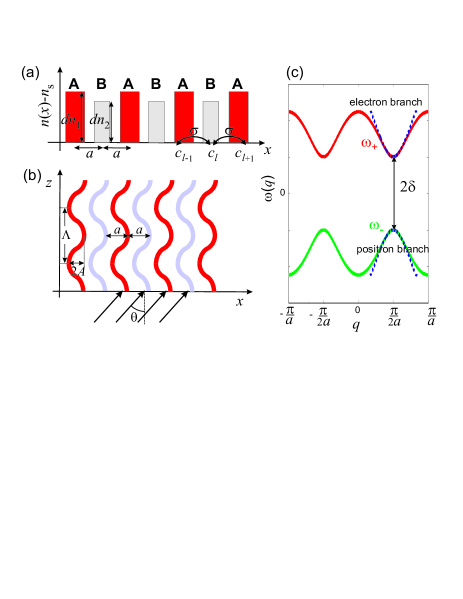
Figure 1: (color online) (a) and (b) Schematic of a binary superlattice, made of two interleaved lattices A and B of waveguides with high ($dn_{1}$) and low ($dn_{2}$) refractive index changes, equally spaced by $a$ [Fig.1(a)] and with a periodically-curved axis [Fig.1(b)]. The array is excited by a broad beam tilted at the angle $\theta$. (c) Dispersion curves (minibands) of the tight-binding binary superlattice [Eq.(3)] for the straight binary array (solid curves), and corresponding electron and positron dispersion curves of the Dirac equation (7) (in absence of the ac field) near the Brillouin zone edge $q=\pi/(2a)$ (dotted curves).

where $q$ is the wave number.

II.2 Quantum-optical analogy

In Ref.Longhi09un , it was recently shown that, near the Brillouin zone edge $q=\pm\pi/(2a)$, the dispersion relations (3) of the straight superlattice approximate the positive (electron) and negative (positron) energy curves of a one-dimensional massive Dirac electron in absence of external fields, and that beam propagation at incidence angles near the Bragg angle mimics the temporal dynamics of a one-dimensional free Dirac electron, the two components of the spinor wave function corresponding to the occupation amplitudes in the two sublattices A and B of the superlattice. To study the photonic analogue of vacuum decay and electron-positron production arising from an oscillating field, we consider here light propagation in a periodically-curved binary array within the tight-binding model (2). As it will be shown below, the undulation of the waveguide axis along the propagation direction mimics an external ac electric field in the one-dimensional Dirac equation. To explain the quantum-optical analogy, let us set in Eqs.(2) $c_{l}(z)=a_{l}(z)\exp[-i\Phi(z)l]$, where

$$\Phi(z)=\int_{0}^{z}d\xi F(\xi)=\frac{2\pi n_{s}a\dot{x}_{0}(z)}{\lambda}.$$ (4)

Coupled-mode equations than take the equivalent form

$$i\frac{da_{l}}{dz} = -\sigma\exp[-i\Phi(z)]a_{l+1}-\sigma\exp[i\Phi(z)]a_{l-1}$$ (5)

$$+ (-1)^{l}\delta a_{l}.$$

Note that, for the special case of a sinusoidal axis bending profile $x_{0}(z)=-A\cos(2\pi z/\Lambda)$ of amplitude $A$ and period $\Lambda$, one has $\Phi(z)=\Phi_{0}\sin(2\pi z/\Lambda)$ with

$$\Phi_{0}=\frac{4\pi^{2}n_{s}aA}{\lambda\Lambda}.$$ (6)

Let us then introduce the following two assumptions: (i) the amplitude of axis bending profile is small enough that $|\Phi|\ll\pi/2$ over the entire oscillation cycle; (ii) the array is excited by a broad beam tilted at the Bragg angle $\theta_{B}=\lambda/(4n_{s}a)$. The first assumption enables to set $\exp(\pm i\Phi)\sim 1\pm i\Phi$ in Eqs.(5); the second assumption implies that the modes in adjacent waveguides are excited with a nearly equal amplitude but with a phase difference of $\pi/2$ Longhi09un . Therefore, after setting $a_{2l}(z)=(-1)^{l}\psi_{1}(l,z)$, $a_{2l-1}=-i(-1)^{l}\psi_{2}(l,z)$, the amplitudes $\psi_{1}$ and $\psi_{2}$ vary slowly with $l$, and one can thus write $\psi_{1,2}(l\pm 1,z)=\psi_{1,2}(l,z)\pm(\partial\psi_{1,2}/\partial l)$ and consider $l\equiv\xi=x/(2a)$ as a continuous variable rather than as an integer index. Under such assumptions, from Eqs.(5) it readily follows that the two-component spinor $\psi(\xi,z)=(\psi_{1},\psi_{2})^{T}$ satisfies the one-dimensional Dirac equation in presence of an external ac field, namely

$$i\frac{\partial\psi}{\partial z}=-i\sigma\alpha\frac{\partial\psi}{\partial\xi}-2\sigma\Phi(z)\alpha\psi+\delta\beta\psi,$$ (7)

where

$$\alpha=\left(\begin{array}[]{cc}0&1\\ 1&0\end{array}\right)\;,\;\beta=\left(\begin{array}[]{cc}1&0\\ 0&-1\end{array}\right)$$ (8)

are the $\sigma_{x}$ and $\sigma_{z}$ Pauli matrices, respectively. Note that, after the formal change

$$\sigma \rightarrow c$$

$$\delta \rightarrow \frac{mc^{2}}{\hbar}$$

$$\xi \rightarrow x$$ (9)

$$\Phi \rightarrow \frac{eA_{x}}{2\hbar c}$$

$$z \rightarrow t,$$

Eq.(7) corresponds to the one-dimensional Dirac equation for an electron of mass $m$ and charge $e$ in presence of a spatially-homogeneous and time-varying vectorial potential $\mathbf{A}=(A_{x},0,0)$, which describes the interaction of the electron with an external oscillating electric field $E_{x}(t)=-(\partial A_{x}/\partial t)$ in the dipole approximation (see, for instance, book ). Note also that, in our optical analogue, the temporal evolution of the spinor wave function $\psi$ for the Dirac electron is mapped into the spatial evolution of the field amplitudes $\psi_{1}$ and $\psi_{2}$ along the $z$-axis of the array, and that the two components $\psi_{1}$, $\psi_{2}$ of the spinor wave function correspond to the occupation amplitudes in the two sublattices A and B composing the superlattice. In absence of the external field, the energy-momentum dispersion relation $\hbar\omega(k)$ of the Dirac equation (7), obtained by making the Ansatz $\psi\sim\exp(ik\xi-i\omega z)$, is composed by the two branches $\omega_{\pm}(k)=\pm\epsilon(k)$, corresponding to positive and negative energy states of the relativistic free electron, where

$$\epsilon(k)=\sqrt{\delta^{2}+\sigma^{2}k^{2}}.$$ (10)

Note that such two branch curves are readily obtained from Eq.(3) after setting

$$q=\frac{\pi}{2a}+\frac{k}{2a}$$ (11)

and assuming small values of $k$, which corresponds to the assumption of slowly-varying envelopes $\psi_{1,2}(l,z)$. Therefore, the positive and negative energy states of the free Dirac electron are mapped into the dispersion curves of the two minibands of the binary array near the boundary of the Brillouin zone at $q=\pi/(2a)$, as shown in Fig.1(c).

III Optical analogue of pair production in an oscillating field

The phenomenon of vacuum decay by oscillating fields, originally predicted in Ref.Brezin70 , refers to the electron-positron pair production due to the instability of the QED vacuum in a superstrong field of two counterpropagating laser beams oscillating2 ; oscillating3 . Vacuum decay should be generally investigated in the framework of a quantum field theory of the Dirac equation, however a simpler and more intuitive approach is possible within the one-particle Dirac equation (7), where pair production corresponds to a field-induced transition of an electron in the Dirac sea of negative-energy states to a final positive-energy state oscillating2 ; oscillating3 . In this approach, a simple picture of pair production as a wave packet break-up process has been suggested oscillating3 . Here an electron in the negative sea is represented by a Gaussian wave packet formed by a superposition of negative-energy states. When the $e^{+}e^{-}$ pair is produced under the action of the oscillating field, a droplet is separated from the wave packet and moves opposite to the initial one (see, for instance, Fig.1 of Ref.oscillating3 ). The droplet is a positive-energy state and represents the created electron. It has been shown that such a simplified model of pair production, besides to be rather intuitive, also provides a correct way to calculate the rate of particle creation oscillating3 . Our classical wave optics analogue, grounded on the formal analogy between the one-particle Dirac equation and the spinor-like wave equation (7) via the variable transformation (9), thus enables to visualize in space the analogue of pair production as a break up of an initial Gaussian wave packet, composed by a superposition of Bloch modes of the lowest lattice miniband and representing an electron in the Dirac sea, under the influence of an oscillating electric field.

III.1 Two-level model

For a spatially-homogeneous and time-dependent field, it is known that momentum conservation reduces the problem of pair creation to a two-level system consisting of a negative and a positive energy state coupled by the external field. Within the two-level model, pair production generally occurs as a multiphoton resonance process enforced by energy conservation, with interesting effects such as Rabi oscillations of the quantum vacuum (see, for instance, oscillating2 ; oscillating3 ). The two-level description of pair production in the dipole approximation for the one-particle Dirac equation can be found, for instance, in Refs.oscillating2 ; for the sake of completeness, it is briefly reviewed in the Appendix for the case of the one-dimensional Dirac equation. Owing to the quantum-optical analogy established in Sec.II.B, the same dynamical scenario is thus expected for light transport in a periodically-curved tight-binding binary array. To this aim, let us look for a solution to coupled-mode equations (5) of the form

$$a_{l}(z)=\left(\begin{array}[]{c}s_{1}(z)\\ s_{2}(z)\end{array}\right)\exp(iqla)$$ (12)

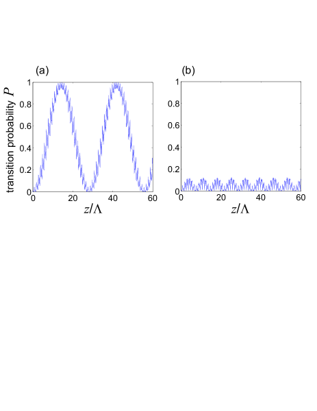
Figure 2: (color online) Transition probability $P=|r_{+}(z)|^{2}$ versus propagation distance $z$, normalized to the ac oscillation period $\Lambda$, in a tight-binding binary lattice with a sinusoidally-curved axis for parameter values $\sigma=2$, $\delta=1.817$, $qa=\pi/4$, $\Phi_{0}=0.4$ and for two values of modulation period $\Lambda$: (a) $\Lambda=2.8556$, and (b) $\Lambda=2.7196$. In (a) the multiphoton resonance condition (22) is satisfied for $n=3$, and Rabi flopping is clearly observed. In (b) the modulation period is slightly decreased by $5\%$ from the $n=3$ resonance value.

where the wave number $q$ is related to the electron momentum $k$ for the Dirac equation (7) by Eq.(11), and where the upper (lower) row applies to an even (odd) value of index $l$. Substitution of Eq.(12) into Eq.(5) yields the following coupled equations

$$i\frac{d}{dz}\left(\begin{array}[]{c}s_{1}\\ s_{2}\end{array}\right)=\mathcal{T}(z)\left(\begin{array}[]{c}s_{1}\\ s_{2}\end{array}\right)$$ (17)

where

$$\mathcal{T}(z)=\left(\begin{array}[]{cc}\delta&-2\sigma\cos[qa-\Phi(z)]\\ -2\sigma\cos[qa-\Phi(z)]&-\delta\end{array}\right).$$ (18)

For a straight array, i.e. in absence of the external field $\Phi=0$, the (normalized) eigenvectors of the $z$-independent matrix $\mathcal{T}$,

$$\left(\begin{array}[]{c}s_{1}\\ s_{2}\end{array}\right)_{\pm}=\left(\begin{array}[]{c}-\frac{2\sigma\cos(qa)}{\sqrt{2|\omega_{\pm}(q)||\omega_{\pm}(q)-\delta|}}\\ \frac{\omega_{\pm}(q)-\delta}{\sqrt{2|\omega_{\pm}(q)||\omega_{\pm}(q)-\delta|}}\end{array}\right),$$ (19)

corresponding to the eigenvalues $\omega_{\pm}(q)$ defined by Eq.(3), belong to the positive (electron) and negative (positron) energy branches. These states are basically the Bloch modes of the superlattice, belonging to the first two lowest bands, with wave number $q$. If the initial state at $z=0$ is prepared in the Bloch mode belonging to the negative energy branch (corresponding to an electron occupying a negative energy state of the Dirac sea in the quantum mechanical context), i.e. if $(s_{1},s_{2})^{T}=(s_{1},s_{2})_{-}^{T}$ at $z=0$, the application of the oscillating external field $\Phi(z)$ can induce a transition to the Bloch mode $(s_{1},s_{2})_{+}^{T}$ on the positive energy branch, i.e. the optical analogue of an electron-positron pair production is realized. It should be noted that direct (and even indirect) interband transitions and Rabi oscillations induced by a suitable longitudinal refractive index modulation in singly-periodic waveguide arrays have been recently predicted and experimentally observed in Refs.SegevRabi , however in those previous works the transitions are not described in terms of a Dirac-type equation with an oscillating field, and the quantum-optical analogy is thus not evident note2 .
To study the field-induced transition process, it is worth projecting the state $(s_{1},s_{2})$ onto the Bloch mode basis (15), i.e. let us set

$$\left(\begin{array}[]{c}s_{1}\\ s_{2}\end{array}\right)=r_{-}(z)\left(\begin{array}[]{c}s_{1}\\ s_{2}\end{array}\right)_{-}+r_{+}(z)\left(\begin{array}[]{c}s_{1}\\ s_{2}\end{array}\right)_{+}$$ (20)

where $r_{-}(z)$ and $r_{+}(z)$ are the occupation amplitudes of the negative and positive electron branches, respectively. Substitution Eq.(16) into Eq.(13) yields the following coupled equations for the occupation amplitudes

$$i\frac{d}{dz}\left(\begin{array}[]{c}r_{-}\\ r_{+}\end{array}\right)=\mathcal{Z}(z)\left(\begin{array}[]{c}r_{-}\\ r_{+}\end{array}\right)$$ (25)

where the $z$-varying elements of the $2\times 2$ matrix $\mathcal{Z}(z)$ are given by

$$\mathcal{Z}_{11} = -\mathcal{Z}_{22}=\frac{\delta^{2}+4\sigma^{2}\cos(qa)\cos[qa-\Phi(z)]}{\omega_{+}(q)}$$ (26)

$$\mathcal{Z}_{12} = \mathcal{Z}_{21}=\frac{2\sigma\delta\left\{\cos(qa)-\cos[qa-\Phi(z)]\right\}}{\omega_{+}(q)}.$$ (27)

Equations (17) are generally encountered in problems of driven two-level systems, and therefore phenomena like population Rabi flopping, multiphoton resonances, etc. are expected to occur in our system as well. Note that the conservation of population implies that $|r_{-}(z)|^{2}+|r_{+}(z)|^{2}=1$. For the initial condition $r_{-}(0)=1$ and assuming that the external ac field is switched on at $z=0$ and off after a propagation distance $z=L_{0}$ (which is assumed to be an integer multiple of the modulation cycle $\Lambda$), i.e. $\Phi(z)=0$ for $z>L_{0}$, the transition probability is thus given by $P=|r_{+}(L_{0})|^{2}$. The connection between the two-level model (17), derived from the tight-binding lattice model (5), and the two-level model of pair production in the framework of the one-dimensional Dirac equation (7) is discussed in the Appendix. The latter model is retrieved from the former one by assuming a wave number $q$ near the edge of the Brilluoin zone [Eq.(11) with $|k|\ll\pi/2$] and a small value of $|\Phi(z)|$; in this case, the expressions of matrix coefficients take the following simplified form [see also Eqs.(A9) and (A10) given in the Appendix]

$$\mathcal{Z}_{11} = -\mathcal{Z}_{22}=\epsilon(k)-\frac{2\sigma^{2}k\Phi(z)}{\epsilon(k)}$$ (28)

$$\mathcal{Z}_{12} = \mathcal{Z}_{21}=-\frac{2\sigma\delta\Phi(z)}{\epsilon(k)}$$ (29)

where $\epsilon(k)$ is defined by Eq.(10). It is worth noticing that, under such an assumption, Eqs.(17) are analogous to the two-level equations describing population dynamics in a two-level dipolar molecule under an external ac field (see, for instance, Longhi06JPB ).
In the context of field-induced pair production, the photon energy $2\pi\hbar/\Lambda$ of the ac field is generally much smaller that the energy separation $2mc^{2}$ between negative and positive energy states, and the transition of one electron out of the Dirac sea into a positive-energy state generally occurs via a multiphoton resonant process (see, for instance, oscillating2 ; oscillating3 ). The condition of $n$-photon resonance, obtained in the low ac frequency limit by a WKB analysis of Eqs.(17-19), reads explicitly (see, e.g., oscillating3 )

$$n\frac{2\pi}{\Lambda}=2\mathcal{E}(q),$$ (30)

where the quasi-energy $\mathcal{E}(q)$ is calculated as

$$\mathcal{E}(q) = \frac{1}{\Lambda}\int_{0}^{\Lambda}dz\sqrt{Z_{11}^{2}(z)+Z_{12}^{2}(z)}$$

$$= \frac{1}{2\pi}\int_{0}^{2\pi}dy\sqrt{\delta^{2}+4\sigma^{2}\cos^{2}[qa-\Phi(\Lambda y/2\pi)]}.$$

As an example, Fig.2(a) depicts the behavior of the transition probability $P=|r_{+}(z)|^{2}$ versus $z$, showing multiphoton Rabi oscillations, as obtained by numerical simulations of Eqs.(17-19) for a sinusoidal ac field $\Phi(z)=\Phi_{0}\sin(2\pi z/\Lambda)$ for parameter values $\sigma=2$, $\delta=1.817$, $qa=\pi/4$, $\Phi_{0}=0.4$ and for a modulation period $\Lambda=2.8556$, which satisfies the multiphoton resonance condition (22) with $n=3$. For comparison, Fig.2(b) shows the behavior of the transition probability for the same parameter values, but for a modulation period $\Lambda=2.7196$ which is $5\%$ smaller than the resonant value of Fig.2(a). A comparison of Figs.2(a) and (b) clearly indicates that, as it is well known, multiphoton pair production is a resonant process.
In our photonic system, the constraints of low modulation frequency and low field amplitudes typical of laser-driven QED vacuum can be overcome. For typical geometrical settings which apply to binary waveguide arrays and for reasonable propagation lengths achievable with current samples, the regimes of fast modulation frequencies (i.e., short bending periods $\Lambda$) and strong amplitudes are indeed more accessible than the low-frequency multiphoton resonance regime; on the other hand, such a latter regime might be accessible for cold atoms in optical superlattices Breid . For instance, the values of $\sigma$ and $\delta$ used in Fig.2 correspond to the coupling rate and propagation constant mismatch, in units of ${\rm cm}^{-1}$, of a typical binary waveguide array for parameters values discussed in the next subsection. For such an array, the modulation period of axis bending in Fig.2(a) that achieves the $n=3$ photon resonance condition is $\Lambda=2.8556$ cm, and the multiphoton Rabi oscillation period shown in Fig.2(a) would thus correspond to about $80$ cm, a length which is not accessible in an experiment. Conversely, the regimes of fast modulation frequency and strong bending amplitudes are easily accessible. In such regimes, efficient transition can occur even for a single-cycle of the ac field [$\Phi(z)=\Phi_{0}\sin(2\pi z/\Lambda)$ for $0<z<\Lambda$, $\Phi(z)=0$ for $z<0$ and $z>\Lambda$], corresponding to the use of ultrastrong single-cycle counter-propagating laser pulses in the QED context. As an example, Fig.3(a) shows the behavior of the transition probability $P$, after the interaction with a single-cycle pulse, as obtained by numerical simulations of Eqs.(17-19) for $\sigma=2$, $\delta=1.817$, $qa=\pi/4$ (as in Fig.2) but with a much shorter period $\Lambda=0.6676$, and for increasing values of the the field amplitude $\Phi_{0}$. Examples of the detailed behavior of $P(z)=|r_{+}(z)|^{2}$ along the oscillation cycle, corresponding to $\Phi_{0}=4$ and $\Phi_{0}=6$ [points A and B in Fig.3(a)], are depicted in Figs.3(b) and (c), respectively.

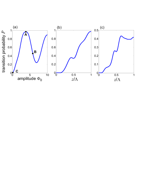
Figure 3: (color online) Transition probability $P$ in a tight-binding binary lattice with a single-cycle sinusoidally-curved axis for parameter values $\sigma=2$, $\delta=1.817$, $qa=\pi/4$, $\Lambda=0.6676$, and for increasing values of amplitude $\Phi_{0}$. Points A, B and C in the figure correspond to the values $\Phi_{0}=4$, $\Phi_{0}=6$ and $\Phi_{0}=0$, respectively. (b) and (c) show the detailed behavior of $|r_{+}(z)|^{2}$ versus propagation distance $z$ in the single-cycle modulation period corresponding to points A [Fig.3(b)] and B [Fig.3(c)] of Fig.3(a).

III.2 Wave packet dynamics

The two-level description of pair production in a spatially-homogeneous and oscillating field described in the previous subsection assumes states with definite momentum $p$ in the negative and positive energy branches, and thus fully delocalized in space. A better visualization of the pair creation process is attained by considering, as an initial state, a free wave packet in the negative-energy continuum (for instance Gaussian-shaped), representing an electron in the Dirac sea oscillating3 . After the external ac field is switched on for some interval (for instance for one oscillation cycle) and then switched off again, transitions into the positive-energy continuum is visualized as a break up of the initial wave packet into two wave packets, which propagates with different group velocities and thus separate in space after some time oscillating3 . These two wave packets represent the amplitude probabilities for the electron to be excited in the positive-energy continuum or to remain in the Dirac sea. In our photonic analogue, wave packet break up is simply explained because of the different refraction angles of wave packets belonging to the two minibands of the superlattices: the creation of a wave packet in the upper lattice miniband, induced by the longitudinal bending of the waveguide axis, is simply observed as a deviation of the propagation direction from that of the initial wave packet.
We have checked such a scenario by direct numerical simulations of the paraxial field equation (1) using a standard pseudospectral split-step method. Parameter values and refractive index profiles used in the simulations are compatible with binary wavegude arrays realized in fused silica by femtosecond laser writing and excited in the visible at $\lambda=633$ nm Dreisow09 .

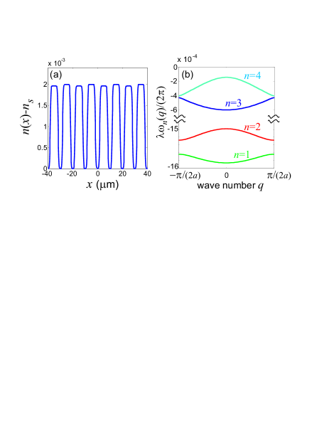
Figure 4: (color online) (a) Refractive index profile of the binary superlattice used in numerical simulations, and (b) corresponding band diagram. Parameter values are given in the text.

Figure 4(a) shows the index profile $n(x)$ of the superlattice used in the simulations, corresponding to a waveguide spacing $a=10\;\mu$m, refractive index changes $dn_{1}=0.002$ and $dn_{2}=0.00196$ of adjacent waveguides, and a substrate refractive index $n_{s}=1.42$. Figure 4(b) shows the dispersion curves $\omega_{n}(q)$ of a few low-order bands of the straight superlattice (band diagram). $\omega_{n}(q)$ are computed by a standard plane-wave expansion method by looking for a solution to Eq.(1), with $F=0$, of Bloch-Floquet type, i.e. of the form $E(x,z)=u_{n}(x,q)\exp(iqx)\exp[-i\omega_{n}(q)z]$, where $n$ is the band order, $q$ varies in the first Brillouin zone $-\pi/(2a)<q\leq\pi/(2a)$, and $u_{n}(x,q)$ in the periodic part of the Bloch mode [$u_{n}(x+2a,q)=u_{n}(x,q)$]. Note that the two lowest bands $n=1$ and $n=2$ in Fig.4(b) correspond to the two minibands $\omega_{-}$ and $\omega_{+}$, respectively, of the tight-binding model (2) depicted in Fig.1(c), i.e. to the negative- and positive-energy branches of the Dirac equation (7) in absence of the external field. For the binary array of Fig.4, the coupling rate $\sigma$ and propagation constant mismatch $\delta$ entering in the tight-binding model (2) can be simply estimated by fitting the two lowest bands of Fig.4(b) using Eq.(3) with $\sigma$ and $\delta$ as fitting parameters, yielding $\sigma\simeq 2\;{\rm cm}^{-1}$ and $\delta\simeq 1.817\;{\rm cm}^{-1}$. To visualize the optical analogue of pair production, the bending profile of the waveguide axis is designed to simulate the action of a single-cycle ultrastrong field in the QED context, namely $x_{0}(z)=-A\cos(2\pi z/\Lambda)$ for $0<z<\Lambda$, and $x_{0}(z)=-A$ for $z>\Lambda$. The array is excited at the input plane by a broad Gaussian beam of spot size $w_{0}$, tilted at the angle $\theta$, i.e. Eq.(1) is integrated with the initial condition $E(x,0)=\exp[-(x/w_{0})^{2}]\exp(2\pi in_{s}x\theta/\lambda)$. The tilt angle has been chosen half of the Bragg angle, i.e. $\theta=\theta_{B}/2$, where $\theta_{B}\simeq 0.64^{\rm o}$. At such a relatively small excitation angle, the lowest band of the array is mostly excited (see, for instance, Longhi06OL ), and therefore the Gaussian wave packet mimics an initial electron wave packet of the Dirac sea, i.e. in the negative-energy spectrum. For $\theta=\theta_{B}/2$, the condition $qa=\pi/4$ of Fig.3 is also satisfied. The modulation period has been set equal to $\Lambda\simeq 0.67$ cm to reproduce the conditions of Fig.3.

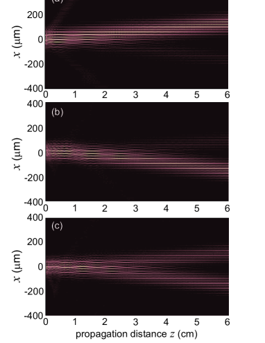
Figure 5: (color online) Beam propagation in a 6-cm-long one-dimensional binary waveguide array (snapshot of $|E(x,z)|^{2}$), comprising a first section with a single-cycle sinusoidally curved axis of period $\Lambda=6.67\;{\rm}$ and amplitude $A$, and a second section with a straight axis: (a) $A=0$ (straight array), (b) $A=30\;\mu$m, and (c) $A=45\;\mu$m The array is excited by a Gaussian beam tilted at half of the Bragg angle (parameter values are given in the text).

Figure 5 shows a few examples of beam propagation along a 6-cm-long array for an initial beam spot size $w_{0}=80\;\mu$m and for increasing values of the modulation amplitude $A$. In Fig.5(a), the array is straight [$A=0$, corresponding to point C of Fig.3(a)] and the wave packet propagates weakly diffracting with a nonvanishing transverse group velocity along a direction which is determined by the normal to the band dispersion curve at $qa=\pi/4$. In Fig.5(b), the amplitude of the modulation is increased to $A=30\;\mu$m, corresponding to $\Phi_{0}\simeq 4$ [see Eq.(6)], i.e. to point A of Fig.3(a). In this case, after the ac field is switched off at $z=\Lambda\simeq 6.7$ mm, the wave packet does not basically break down, however it is now refracted in an opposite direction as compared to the case of Fig.5(a). This is the clear signature that the wave packet is mostly composed by Bloch modes of the second band, i.e. that an almost complete transition from negative- to positive-energy states has occurred, according to the predictions of the two-level analysis [see point A of Fig.3(a)]. In Fig.5(c), the amplitude of the modulation is further increased to $A=45\;\mu$m, corresponding to $\Phi_{0}\simeq 6$. According to the prediction of the two-level analysis [see point B of Fig.3(a)], after the ac field is switched off the transition probability for the wave packet components is $\sim 45\%$. Accordingly, the wave packet breaks up at propagation distances $z>\Lambda$, with the two nearly balanced wave packets belonging to the first and second array minibands refracting along two opposite directions.

IV Conclusions

Vacuum decay and electron-positron pair production due to the instability of the QED vacuum in an external oscillating field are remarkable predictions of the Dirac theory. Their experimental demonstration, however, requires ultrastrong and high-frequency laser fields which are not yet available. In this work a classic wave optics analogue of vacuum decay has been proposed which is based on the formal analogy between the temporal dynamics of the one-dimensional Dirac equation for a single particle in an external spatially-homogeneous oscillating field and the spatial propagation of monochromatic light waves in a periodically-curved binary waveguide array. Our photonic analogue enables a simple and experimentally-accessible visualization in space of the process of pair production as break up of an initially negative-energy Gaussian wave packet, representing an electron in the Dirac sea, under the influence of an oscillating electric field.

Appendix A Two-level description of pair production in the dipole approximation

In this Appendix we briefly review the two-level description of pair production, induced by an oscillating field in the dipole approximation, for the one-dimensional single-particle Dirac equation given by Eq.(7) in the text. In making such an analysis, we introduce the variable transformation defined by Eqs.(9), and re-write Eq.(7) into the more familiar quantum mechanical form

$$i\hbar\frac{\partial\psi}{\partial t}=(cp_{x}-eA_{x})\alpha\psi+mc^{2}\beta\psi,$$ (32)

where $p_{x}=-i\hbar\partial_{x}$. The independence of the vectorial potential $A_{x}$ on the spatial coordinate $x$ corresponds to the electric dipole approximation and to the interaction with a spatially-homogeneous oscillating electric field. Owing to the pure time dependence of the external potential, the momentum is conserved during the transition. Therefore only transitions between negative- and positive-energy states with the same momentum are permitted in the pair creation process. Indicating by $p=\hbar k$ the momentum of the particle at initial time, a solution to Eq.(7) with definite momentum is given by

$$\psi(x,t)=\varphi(t)\exp(ikx)$$ (33)

where the two-component spinor $\varphi=(\varphi_{1},\varphi_{2})^{T}$ satisfies the equation

$$i\frac{d\varphi}{dt}=\mathcal{M}(t)\varphi.$$ (34)

The time-dependent elements of the $2\times 2$ matrix $\mathcal{M}$ in Eq.(A3) are given by

$$\mathcal{M}_{11} = -\mathcal{M}_{22}=\frac{mc^{2}}{\hbar}$$ (35)

$$\mathcal{M}_{12} = \mathcal{M}_{21}=kc-\frac{eA_{x}(t)}{\hbar}.$$ (36)

To investigate field-induced transitions, let us project the spinor $\varphi(t)$ on the basis of the two eigenstates $\varphi_{\pm}$ of the free electron (i.e., in the absence of the external field) corresponding to the negative and positive energy branches, i.e. let us set

$$\varphi(t)=r_{-}(t)\varphi_{-}+r_{+}(t)\varphi_{+}$$ (37)

where

$$\varphi_{\pm}=\frac{1}{\sqrt{p^{2}c^{2}+[\hbar\epsilon(p)\mp mc^{2}]^{2}}}\left(\begin{array}[]{c}cp\\ \pm\hbar\epsilon(p)-mc^{2}\end{array}\right),$$ (40)

$\hbar\epsilon(p)=\sqrt{p^{2}c^{2}+(mc^{2})^{2}}$, and $r_{\pm}(t)$ are the occupation amplitudes of negative and positive energy states at time $t$. The amplitudes $r_{-}(t)$ and $r_{+}(t)$ then satisfy the coupled equations of driven two-level systems

$$i\frac{d}{dt}\left(\begin{array}[]{c}r_{-}\\ r_{+}\end{array}\right)=\mathcal{Z}(t)\left(\begin{array}[]{c}r_{-}\\ r_{+}\end{array}\right)$$ (41)

with matrix elements given by

$$\mathcal{Z}_{11} = -\mathcal{Z}_{22}=\epsilon(p)-\frac{pceA_{x}(t)}{\hbar^{2}\epsilon(p)}$$ (42)

$$\mathcal{Z}_{12} = \mathcal{Z}_{21}=-\frac{mc^{2}eA_{x}(t)}{\hbar^{2}\epsilon(p)}.$$ (43)

Equations (A8-A10) are analogous to Eqs.(17-19) given in text for the driven tight-binding lattice (5). In particular, according to the approximations used to derive the Dirac equation (7) in Sec.II.B, the expressions of the matrix coefficients $\mathcal{Z}_{ik}(t)$, defined by Eqs.(18) and (19), reduce to those given by Eqs.(A9) and (A10), after the replacement $qa\rightarrow\pi/2+k/2$ [see Eq.(11)], assuming $|k|\ll\pi/2$, and using the transformation of variables (9) that connect the quantum and optical descriptions.

References

- (1) D. Dragoman and M. Dragoman, Quantum-Classical Analogies (Springer, Berlin, 2004).
- (2) S. Longhi, Laser & Photon. Rev. 3, 243 261 (2009).
- (3) D. N. Christodoulides, F. Lederer, and Y. Silberberg, Nature 424, 817 (2003).
- (4) U. Peschel, T. Pertsch, and F. Lederer, Opt. Lett. 23, 1701; R. Morandotti, U. Peschel, J. S. Aitchison, H. S. Eisenberg, and Y. Silberberg, Phys. Rev. Lett. 83, 4756 (1999); T. Pertsch, P. Dannberg, W. Elflein, A. Bräuer, and F. Lederer, Phys. Rev. Lett. 83, 4752 (1999); G. Lenz, I. Talanina, and C.M. de Sterke, Phys. Rev. Lett. 83, 963 (1999); N. Chiodo, G. Della Valle, R. Osellame, S. Longhi, G. Cerullo, R. Ramponi, P. Laporta, and U. Morgner, Opt. Lett. 31, 1651 (2006); H. Trompeter, W. Krolikowski, D. N. Neshev, A. S. Desyatnikov, A.A. Sukhorukov, Yu. S. Kivshar, T. Pertsch, U. Peschel, and F. Lederer, Phys. Rev. Lett. 96, 053903 (2006).
- (5) R. Khomeriki and S. Ruffo, Phys. Rev. Lett. 94, 113904 (2005); H. Trompeter, T. Pertsch, F. Lederer, D. Michaelis, U. Streppel, A. Bräuer, and U. Peschel, Phys. Rev. Lett. 96, 023901 (2006); A. Fratalocchi, G. Assanto, K. A. Brzdakiewicz, and M. A. Karpierz, Opt. Lett. 31, 1489 (2006); A. Fratalocchi and G. Assanto, Opt. Express 14, 2021 (2006); S. Longhi, Europhys. Lett. 76, 416 (2006).
- (6) F. Dreisow, A. Szameit, M. Heinrich, T. Pertsch, S. Nolte, A. Tünnermann, and S. Longhi, Phys. Rev. Lett. 102, 076802 (2009).
- (7) S. Longhi, Opt. Lett. 30, 2137 (2005); S. Longhi, M. Marangoni, M. Lobino, R. Ramponi, P. Laporta, E. Cianci, and V. Foglietti, Phys. Rev. Lett. 96, 243901 (2006); R. Iyer, J. S. Aitchison, J. Wan, M. M. Dignam, and C. M. de Sterke, Opt. Express 15, 3212 (2007); F. Dreisow, M. Heinrich, A. Szameit, S. Döring, S. Nolte, A. Tünnermann, S. Fahr, and F. Lederer, Opt. Express 16, 3474 (2008); A. Szameit, I.L. Garanovich, M. Heinrich, A.A. Sukhorukov, F. Dreisow, T. Pertsch, S. Nolte, A. Tünnermann, and Y.S. Kivshar, Nature Phys. 5, 271 (2009); A. Joushaghani, R. Iyer, J.K.S. Poon, J.S. Aitchison, C.M. de Sterke, J. Wan, and M.M. Dignam, Phys. Rev. Lett. 103, 143903 (2009).
- (8) I. Vorobeichik, E. Narevicius, G. Rosenblum, M. Orenstein, and N. Moiseyev, Phys. Rev. Lett. 90, 176806 (2003); G. Della Valle, M. Ornigotti, E. Cianci, V. Foglietti, and P. Laporta, and S. Longhi, Phys. Rev. Lett. 98, 263601 (2007); A. Szameit, Y. V. Kartashov, F. Dreisow, M. Heinrich, T. Pertsch, S. Nolte, A. Tünnermann, V. A. Vysloukh, F. Lederer, and L. Torner, Phys. Rev. Lett. 102, 153901 (2009).
- (9) S. Longhi, D. Janner, M. Marano, and P. Laporta, Phys. Rev. E 67, 036601 (2003); S. Longhi, M. Marangoni, D. Janner, R. Ramponi, P. Laporta, E. Cianci, and V. Foglietti, Phys. Rev. Lett. 94, 073002 (2005).
- (10) T. Schwartz, G. Bartal, S. Fishman, and M. Segev, Nature 446, 55 (2007); Y. Lahini, A. Avidan, F. Pozzi, M. Sorel, R. Morandotti, D. N. Christodoulides, and Y. Silberberg, Phys. Rev. Lett. 100, 013906 (2008).
- (11) S. Longhi, Phys. Rev. Lett. 97, 110402 (2006); P. Biagioni, G. Della Valle, M. Ornigotti, M. Finazzi, L. Duó, P. Laporta, and S. Longhi, Opt. Express 16, 3762 (2008); F. Dreisow, A. Szameit, M. Heinrich, T. Pertsch, S. Nolte, A. Tünnermann, and S. Longhi, Phys. Rev. Lett. 101, 143602 (2008).
- (12) E. Paspalakis, Opt. Commun. 258, 31 (2006); S. Longhi, G. Della Valle, M. Ornigotti, and P. Laporta, Phys. Rev. B 76, 201101(R) (2007); Y. Lahini, F. Pozzi, M. Sorel, R. Morandotti, D. N. Christodoulides, and Y. Silberberg, Phys. Rev. Lett. 101, 193901 (2008); F. Dreisow, A. Szameit, M. Heinrich, R. Keil, S. Nolte, A. Tünnermann, and S. Longhi, Opt. Lett. 34, 2405 (2009).
- (13) S. G. Krivoshlykov and I. N. Sissakian, Opt. Quantum Electron. 11, 393 (1979); S. Longhi, Opt. Lett. 34, 2736 (2009).
- (14) K.S. Novoselov, A. K. Geim, S. V. Morozov, D. Jiang, M.I. Katsnelson, I.V. Grigorieva, S.V. Dubonos, and A.A. Firsov, Nature (London) 438, 197 (2005); S.Y. Zhou, G.-H. Gweon, J. Graf, A.V. Fedorov, C.D. Spataru, R.D. Diehl, Y. Kopelevich, D.-H. Lee, Steven G. Louie, and A. Lanzara, Nature Phys. 2, 595 (2006); M.I. Katsnelson, K.S. Novoselov, and A.K. Geim, Nature Phys. 2, 620 (2006).
- (15) C. W. J. Beenakker, Rev. Mod. Phys. 80, 1337 (2008); A. H. Castro Neto, F. Guinea, N. M. Peres, K. S. Novoselov, and A. K. Geim, Rev. Mod. Phys. 81, 109 (2009).
- (16) P.M. Alsing, J.P. Dowling, and G.J. Milburn, Phys. Rev. Lett. 94, 220401 (2005); J. Schliemann, D. Loss, and R.M. Westervelt, Phys. Rev. Lett. 94, 206801 (2005); A. Bermudez, M.A. Martin-Delgado, and E. Solano, Phys. Rev. A 76, 041801(R) (2007); L. Lamata, J. Leon, T. Schatz, and E. Solano, Phys. Rev. Lett. 98, 253005 (2007); G. Juzeliunas, J. Ruseckas, M. Lindberg, L. Santos, and P. Ohberg, Phys. Rev. A 77, 011802(R) (2008); M. Johanning, A. F. Varón, and C. Wunderlich, J. Phys. B 42, 154009 (2009); N. Goldman, A. Kubasiak, A. Bermudez, P. Gaspard, M. Lewenstein, and M.A. Martin-Delgado, Phys. Rev. Lett. 103, 035301 (2009).
- (17) K. Huang, Am. Phys. J. 20, 479 (1952).
- (18) O. Klein, Z. Phys. 53, 157 (1929).
- (19) A. F. Young and P. Kim, Nat. Phys. 5, 222 (2009); N. Stander, B. Huard, and D. Goldhaber-Gordon, Phys. Rev. Lett. 102, 026807 (2009).
- (20) G. A. Steele, G. Gotz and L. P. Kouwenhoven, Nature NanoTechn. 4, 363 (2009).
- (21) F.D.M. Haldane and S. Raghu, Phys. Rev. Lett. 100, 013904 (2008); R.A. Sepkhanov, Ya. B. Bazaliy, and C.W.J. Beenakker, Phys. Rev. A 75, 063813 (2007); O. Peleg, G. Bartal, B. Freedman, O. Manela, M. Segev, and D.N. Christodoulides, Phys. Rev. Lett. 98, 103901 (2007); O. Bahat-Treidel, O. Peleg, and M. Segev, Opt. Lett. 33, 2251 (2008); T. Ochiai and M. Onoda, Phys. Rev. B 80, 155103 (2009).
- (22) X. Zhang, Phys. Rev. Lett. 100, 113903 (2008).
- (23) D.Ö Güney and D.A. Meyer, Phys. Rev. A 79, 063834 (2009); L.-G. Wang, Z.-G. Wang, J.-X. Zhang, and S.-Y. Zhu, Opt. Lett. 34, 1510 (2009); L.-G. Wang, Z.-G. Wang, and S.-Y. Zhu, EPL 86, 47008 (2009).
- (24) S. Longhi, ”Photonic analogue of Zitterbewegung in binary waveguide arrays”, Opt. Lett. (to be published).
- (25) O. Bahat-Treidel, O. Peleg, M. Grobman, N. Shapira, T. Pereg-Barnea, and M. Segev, arXiv:0905.4278v3 (2009).
- (26) E. S. Fradkin, D. M. Gitman, and Sh. M. Shvartsman, Quantum Electrodynamics with Unstable Vacuum (Springer, Berlin, 1991).
- (27) H.K. Avetissian, Relativistic Nonlinear Electrodynamics (Springer, New York, 2006).
- (28) J. Schwinger, Phys. Rev. 82, 664 (1951).
- (29) E. Brezin and C. Itzykson, Phys. Rev. D 2, 1191 (1970).
- (30) V. S. Popov, JETP Lett. 18, 255 (1973); V. M. Mostepanenko and V. M. Frolov, Sov. J. Nucl. Phys. 19, 451 (1974); H. M. Fried, Y. Gabellini, B. H. J. McKellar, and J. Avan, Phys. Rev. D 63, 125001 (2001); D.B. Blaschke, A.V. Prozorkevich, C. D. Roberts, S. M. Schmidt, and S. A. Smolyansky, Phys. Rev. Lett. 96, 140402 (2006); S.S. Bulanov , N.B. Narozhny, V.D. Mur, and V.S. Popov, JETP 102, 9 (2006); Q. Su and R. Grobe, Laser Phys. bf 17, 92 (2007); C.C. Gerry, Q. Su, and R. Grobe, Phys. Rev. A 74, 044103 (2006); R. Schützhold, H. Gies, and G. Dunne, Phys. Rev. Lett. 101, 130404 (2008); F. Hebenstreit, R. Alkofer, G.V. Dunne, and H. Gies, Phys. Rev. Lett. 102, 150404 (2009); T. Cheng, Q. Su, and R. Grobe, Phys. Rev. A 80, 013410 (2009).
- (31) H.K. Avetissian, A.K. Avetissian, G.F. Mkrtchian, and Kh.V. Sedrakian, Phys. Rev. E 66, 016502 (2002); A. Di Piazza, Phys. Rev. D 70, 053013 (2004); I. Tsohantjis, S. Moustaizis, and I. Ploumistakis, Phy. Lett. B 650, 249 (2007); C. Müller, K.Z. Hatsagortsyan, M. Ruf, S.J. Müller, H.G. Hetzheim, M.C. Kohler, and C.H. Keitel, Laser Phys. 19, 1743 (2009).
- (32) M. Ruf, G.R. Mocken, C. Müller, K.Z. Hatsagortsyan, and C.H. Keitel, Phys. Rev. Lett. 102, 080402 (2009). See also: M. Ruf, Ph.D. thesis, Universität Heidelberg, Germany, 2009.
- (33) Experimental observations of the vacuum decay and corresponding pairs creation triggered solely by pure laser light are still lacking, though they may be envisaged in the near future with the development of new ultrastrong laser system facilities.
- (34) S. Longhi, Opt. Lett. 31, 1857 (2006).
- (35) B.M. Breid, D. Witthaut, H.J. Korsch, New J. Phys. 8, 110 (2006); B.M. Breid, D. Witthaut, H.J. Korsch, New J. Phys. 9, 62 (2006); D. Witthaut, E.M. Graefe, S. Wimberger, H.J. Korsch, Phys. Rev. A 75, 013617 (2007); S. Rist, P. Vignolo, and G. Morigi, Phys. Rev. A 79, 053822 (2009).
- (36) W. Greiner, Relativistic Quantum Mechanics (Springer-Verlag, Berlin, 1990), Chapt.2.
- (37) V.S. Shchesnovich and S.Chávez-Cerda, Opt. Lett. 32, 1920 (2007); K.G. Makris, D.N. Christodoulides, O. Peleg, M. Segev, and D. Kip, Opt. Express 16, 10309 (2008); K. Shandarova, C.E. Rüter, D. Kip, K.G. Makris, D.N. Christodoulides, O. Peleg, and M. Segev, Phys. Rev. Lett. 102, 123905 (2009). Rabi oscillations of cold atoms between Bloch bands of a singly-periodic optical lattice were earlier observed in: M. C. Fischer, K. W. Madison, Qian Niu, and M. G. Raizen, Phys. Rev. A 58, R2648 (1998).
- (38) A two-band dynamics in singly-periodic lattices, such as beam propagation involving Bloch modes at the top or at the bottom of two different and well-separated bands near the boundary of the Brillouin zone, is more naturally described by two independent Schrödinger-like equations for the Wannier function envelopes, with different and of opposite sign for the effective masses, rather than by a Dirac equation for a spinor wave function [see, for instance: J. M. Luttinger, Phys. Rev. 84, 814 (1951); J.M. Luttinger and W. Kohn, Phys. Rev. 97, 869 (1955)]. In this case, a two-band tight-binding analysis of Rabi oscillations is generally investigated using a different Hamiltonian than that leading to Eqs.(2) [see, for instance, X.-G. Zhao, G.A. Georgakis, and Q. Niu, Phys. Rev. B 54, (R)5235 (1995)].
- (39) A. Brown, W.J. Meath, and P. Tran, Phys. Rev. A 63, 013403 (2000); O.G. Calderon, S. Melle, and I. Gonzalo, Phys. Rev. A 65, 023811 (2002); S. Longhi, J. Phys. B 39, 1985 (2006).