Mid-infrared spectroscopy of Spitzer-selected ultra-luminous starbursts at z $\sim$ 2

Abstract

Context. Spitzer’s wide-field surveys and followup capabilities have allowed a new breakthrough in mid-IR spectroscopy up to redshifts $\geq 2$, especially for 24 $\mu$m detected sources.

Aims. We want to study the mid-infrared properties and the starburst and AGN contributions, of 24 $\mu$m sources at $z\sim 2$, through analysis of mid-infrared spectra combined with millimeter, radio, and infrared photometry. Mid-infrared spectroscopy allows us to recover accurate redshifts.

Methods. A complete sample of 16 Spitzer-selected sources (ULIRGs) believed to be starbursts at $z\sim 2$ (“5.8 $\mu$m-peakers”) was selected in the (0.5 deg²) J1064+56 SWIRE Lockman Hole field (“Lockman-North”). These sources have $S_{\rm 24\,\mu m}>0.5$ mJy, a stellar emission peak redshifted to 5.8 $\mu$m, and $r^{\prime}_{\rm Vega}>23$. The entire sample was observed with the low resolution units of the Spitzer/IRS infrared spectrograph. These sources have 1.2 mm observations with IRAM 30 m/MAMBO and very deep 20 cm observations from the VLA. Nine of our sources also benefit from 350 $\mu$m observation and detection from CSO/SHARC-II. All these data were jointly analyzed.

Results. The entire sample shows good quality IRS spectra dominated by strong PAH features. The main PAH features at 6.2, 7.7, 8.6, and 11.3 $\mu$m have high S/N average luminosities of $2.90\pm 0.31$, $10.38\pm 1.09$, $3.62\pm 0.27$, and $2.29\pm 0.26\times 10^{10}\,L_{\odot}$, respectively. Thanks to their PAH spectra, we derived accurate redshifts spanning from 1.750 to 2.284. The average of these redshifts is 2.017$\pm$0.038. This result confirms that the selection criteria of “5.8 $\mu$m-peakers” associated with a strong detection at 24 $\mu$m are reliable to select sources at $z\sim 2$. We have analyzed the different correlations between PAH emission and infrared, millimeter, and radio emission. Practically all our sources are strongly dominated by starburst emission, with only one source showing an important AGN contribution. We have also defined two subsamples based on the equivalent width at 7.7 $\mu$m to investigate AGN contributions.

Conclusions. Our sample contains strong starbursts and represents a particularly 24 $\mu$m-bright class of SMGs. The very good correlation between PAH and far-IR luminosities is now confirmed in high-$z$ starburst ULIRGs. These sources show a small AGN contribution to the mid-IR, around $\sim$20% or less in most cases.

1 Introduction

The mid-infrared (MIR) regime is known to provide very rich diagnostics of the interstellar medium (ISM) of galaxies. Hot dust from starbursts and especially AGN contributes to continuum emission. Dust also produces various absorption features, most spectacularly from silicates. However, the MIR spectra of star-forming galaxies are dominated by strong emission features attributed to polycyclic aromatic hydrocarbons (PAHs). These large molecules, typically a few hundred carbon atoms in the ISM, are the carriers of the series of prominent emission bands observed between 3 and 19 $\mu$m, especially between 6 and 12 $\mu$m (Leger & Puget 1984; Allamandola et al. 1985). PAHs efficiently absorb UV and optical photons from young stars and reemit the energy mostly in the mid-infrared.

After their discovery in the local ISM and nearby star-forming regions, PAH features have proved to be common, not only in various regions of the Milky Way, but in other galaxies ranging from local systems to high-$z$ starbursts (e.g., Tielens 2008). PAH features were the focus of a good fraction of the MIR spectroscopy programs of the infrared space observatories ISO and Spitzer. Important key projects of both missions were devoted to MIR spectroscopy of large samples of galaxies. The ISO Key Project on Nearby Galaxies (Helou et al. 2000) showed an amazing similarity of PAH spectra in various galaxy environments. More detailed studies with the SINGS spectral mapping program (Kennicutt et al. 2003) using the Spitzer Infrared Spectrograph (IRS: Houck et al. 2004) provided further evidence of interband PAH feature strength variations, especially in the presence of weak AGN (Smith et al. 2007).

The high sensitivity of Spitzer/IRS allowed the extension of PAH spectroscopy to $z\ga 2$ for samples of hundreds of galaxies that could be observed in the $\sim 5$-35 $\mu$m spectral range. This led to the measurement of a large number of redshifts of dust-enshrouded Spitzer sources at $1.5<z<2.5$ in the so-called “redshift desert” of optical spectroscopy. These MIR spectra allow one to distinguish power-law AGN-dominated spectra from PAH starburst-dominated spectra and composite systems. This long series of high-$z$ IRS studies has thus established the criteria for the identification of various types of sources from Spitzer 3.5-24 $\mu$m photometry (Fadda et al. 2010; Houck et al. 2005; Yan et al. 2005, 2007; Sajina et al. 2007; Weedman et al. 2006; Dasyra et al. 2009; Hernán-Caballero et al. 2009; Bertincourt et al. 2009). Particular types of sources can be selected using various criteria: dust-enshrouded AGN from strong 24 $\mu$m fluxes and/or power-law IRAC 3.6-8.0$\mu$m spectra (Dey et al. 2008; Dey & The Ndwfs/MIPS Collaboration 2009), starbursts from the presence of a visible redshifted 1.6 $\mu$m stellar bump (Farrah et al. 2006, 2008; Lonsdale et al. 2009; Huang et al. 2009; Desai et al. 2009), Type 1 or Type 2 QSOs (Lutz et al. 2008; Martínez-Sansigre et al. 2008), and submillimeter-selected galaxies (SMGs: Valiante et al. 2007; Menéndez-Delmestre et al. 2007, 2009; Pope et al. 2008; Coppin et al. 2010).

Indeed, strong PAH emission is so characteristic of starbursts that the strength of PAH features may be used as a star formation rate indicator. This is justified by the good correlation that has been found between the luminosity of PAH features (mostly at 6.2 and 7.7 $\mu$m) and the total IR or far-IR luminosity, which in the absence of an AGN is taken to be a good tracer of star-forming activity (Kennicutt 1998). Such a correlation has been checked for starburst galaxies at both low and high redshift (e.g., Brandl et al. 2006; Pope et al. 2008; Menéndez-Delmestre et al. 2009). It is the origin of the correlation found between the ISO 7.0 $\mu$m- or Spitzer 8.0$\,\mu$m-band flux and the star formation rate (e.g., Elbaz et al. 2002; Wu et al. 2006; Alonso-Herrero et al. 2006; Farrah et al. 2007) in low-$z$ luminous infrared galaxies. It is similarly related to the use of the single-band 24 $\mu$m luminosity for determining star formation rates of galaxies at high redshift, especially at $z\sim 2$ (e.g., Bavouzet et al. 2008; Rieke et al. 2009; Elbaz 2010, Fiolet et al. in prep.).

Such rich diagnostics of the properties of the ISM and star formation at high redshift provided by mid-IR PAH spectral features have justified the many studies performed with the unique capabilities of Spitzer/IRS. We have used this experience to focus one of the last observations of “cold” Spitzer to obtain high-quality mid-IR spectra of $z\sim 2$ starbursts. Our sample was Spitzer-selected in a field with very rich multiwavelength data. We aimed to select starburst-dominated ultra-luminous IR galaxies at $z\sim 2$ based on the presence of a rest-frame 1.6 $\mu$m stellar bump– caused by the photospheric opacity minimum in giant or supergiant stars (e.g. John 1988; Simpson & Eisenhardt 1999; Weedman et al. 2006)– in the 5.8 $\mu$m IRAC band, together with very strong PAH emission implied by a high 24 $\mu$m flux density. Using these “5.8 $\mu$m-peakers,” we sought to address in the best conditions the various goals allowed by such studies: determination of redshifts from PAH features, accurate enough for allowing CO line observations with current millimeter facilities; detailed examination of the properties of PAH features in such high-$z$ sources, especially their luminosity ratios, and comparison to local systems; estimation of the ratio between PAH bands and the weak underlying continuum that may constrain the modest AGN contribution; and accurate assessment of the correlation of PAH luminosities with total and far-infrared luminosities (and with the radio luminosity). Silicate absorption at 9.7 $\mu$m may provide additional information about the distribution of interstellar dust.

In this paper, we present the observations and the results from IRS spectroscopy of a complete sample of 16 sources selected by their IRAC and MIPS fluxes. The sample selection and the observations are described in Section 2. The method adopted to reduce these observations is presented in Section 3. The results and their analysis are discussed in Sections 4 and 5. In Section 6, we discuss the discrimination between starburst- and AGN-dominated sources, and we make comparisons with the other samples of SMGs. Throughout the paper, we adopt a standard flat cosmology with $H_{0}=71\,{\rm km\,s^{-1}\,Mpc^{-1}}$, $\Omega_{M}=0.27$, and $\Omega_{\Lambda}=0.73$ (Spergel et al. 2003).

2 Sample selection and observations

2.1 Sample selection

Our sample is based on the Spitzer/SWIRE “5.8 $\mu$m-peaker” sample of Fiolet et al. (2009) (hereafter F09). Using the 2007 SWIRE internal catalogue, we have selected the sixteen 24$\,\mu$m-brightest sources of this sample with $S_{\rm 24\,\mu m}>0.5$ mJy. These sources obey the “5.8 $\mu$m-peaker” criteria with $S_{\rm 3.6\,\mu m}<S_{\rm 4.5\,\mu m}<S_{\rm 5.8\,\mu m}>S_{\rm 8.0\,\mu m}$. Some of our sources have no detection in the 8.0 $\mu$m band, but we assume that these sources are also “5.8 $\mu$m-peakers” if their fluxes at 5.8 $\mu$m are greater than the detection limits at 8.0 $\mu$m ($<40$ mJy). To remove low-redshift interlopers, we also require that the sources be optically faint, i.e., $r^{\prime}_{\rm Vega}>23$ (Lonsdale et al. 2006). Our sample is complete for these criteria over 0.5 deg². This area includes the “Lockman-North” field observed with the VLA (Owen & Morrison 2008; Owen et al. 2009) and Herschel (Oliver et al. 2010). For this sample from F09, we have 1.2 mm flux densities ($S_{\rm 1.2\,mm}$) obtained with IRAM/MAMBO [Institut de Radioastronomie Millimétrique/Max-Planck Millimeter Bolometer] array (Kreysa et al. 1998). 62% (10/16) of our sources are detected with S/N $>3$ at 1.2 mm (Table 1) and are thus submillimeter galaxies (SMGs) with $S_{\rm 1.2\,mm}>2\,{\rm mJy}$ ($\langle S_{\rm 1.2\,mm}\rangle=2.72\pm 0.54$ mJy). The six other sources have an average $\langle S_{\rm 1.2\,mm}\rangle=1.01\pm 0.68$ mJy (see Table 1 and F09). This sample is thus representative of a Spitzer-selected subclass of powerful $z\sim 2$ ULIRGs (SMGs and OFRGs, Chapman et al. in prep; Magdis et al. 2010), of which there are $\sim 2000$ in all SWIRE fields that peak at 4.5 or 5.8 $\mu$m and have $S_{\rm 24\,\mu m}>500\,\mu$Jy.

Nine of our sources detected at 1.2 mm were observed at 350 $\mu$m by Kovács et al. (2010). All these sources have been detected, and our 16 sources are also detected at 250 – 350 $\mu$m by Herschel (Fiolet et al. in prep; Magdis et al. 2010). The “5.8 $\mu$m-peaker” criterium also implies that our sample is a mass selected-sample and has $z\sim 2$.

All of our sources benefit from very deep radio data at 1400, 610, and 324 MHz from the VLA and GMRT (Owen & Morrison 2008; Owen et al. 2009, Owen et al. in prep.), with observed flux densities $S_{\rm 20\,cm}>50\,\mu$Jy (Table 1 and F09).

Our sample differs from the other samples of ULIRGs essentially in its selection criteria and redshift range. Indeed, Farrah et al. (2008) and Sajina et al. (2007) have selected bright sources at 24 $\mu$m. However, the sample of Sajina et al. (2007) is built to select the reddest objects in the [$24\,{\rm\mu m}-8\,{\rm\mu m}$] vs. [$24\,{\rm\mu m}-R$] color-color diagram and is composed of PAH-weak and PAH-strong sources. In the comparisons that follow, we consider only the PAH-strong sources of this sample. Pope et al. (2008), Menéndez-Delmestre et al. (2009), and Valiante et al. (2007) have built samples of SMGs detected at 850 $\mu$m. Nevertheless, the sources from Pope et al. (2008) selected with $S_{\rm 24\,\mu m}>200\,\mu$ Jy are fainter than our sources ($S_{\rm 24\,\mu m}>500\,\mu$Jy). Menéndez-Delmestre et al. (2009) and Valiante et al. (2007) have also selected their sample based on 1.4 GHz flux density. The sample of Desai et al. (2009) is relatively similar to ours, with sources selected by a redshifted 1.6 $\mu$m stellar bump in the IRAC bands and $S_{\rm 24\,\mu m}$ $>$ 500 $\mu$Jy. These sources are also optically faint and satisfy the definition of Dust-Obscured Galaxies (DOGs: Dey et al. 2008). The sample of Huang et al. (2009) is also selected with $S_{\rm 24\,\mu m}>500\,\mu$Jy and with color-color criteria yielding star-forming galaxies. Coppin et al. (2010) have built a sample of SMGs selected to be AGN-dominated. While our sample has redshifts from $\sim 1.7$ to $\sim 2.3$, the other samples span larger redshift ranges. Shi et al. (2009) have selected sources at intermediate redshift around $z\sim 1$. Farrah et al. (2008) observed sources with $z=1.3-2.2$ centered at $z\sim 1.7$ (“4.5 $\mu$m-peakers”). The samples of SMGs from Pope et al. (2008); Menéndez-Delmestre et al. (2009) and Valiante et al. (2007), and the DOG sample of Desai et al. (2009), span redshifts from $\sim 1$ to $\sim 3$ (0.6 to 3.6 for Menéndez-Delmestre et al. 2009). The sample of star-forming galaxies of Huang et al. (2009) has redshifts between 1.7 and 2.1 centered at $z\sim 1.9$. Finally, the sample of Coppin et al. (2010) ranges from $z\sim 2.45$ to $\sim 3.4$.

2.2 Observations

The photometric redshifts of our targets, based on the IRAC bands, lie in the range $z\sim 1.5-2.7$ with uncertainties of $\pm 0.5$ (see F09). In this redshift range, the low-resolution ($R\sim 60-127$) Long-Low observing modules of IRS, LL1 (19.5$-$38.0 $\mu$m) and LL2 (14.0$-$21.3 $\mu$m), can cover most of the PAH emission features from 6.2 to 11.3 $\mu$m in the rest frame. Indeed, the actual redshifts have all proved to lie in the range $1.7<z<2.3$ (see Sec. 4.1).

This project (GO50119, PI G. Lagache) was observed for a total time of 53 hours (41 hours on-source) during the last cold campaign of Spitzer, on January 20-22, 2009. We have divided our sample into four groups based on 24$\,\mu$m flux density. For each group, the on-target exposure time is summarized in Table 2. We chose these exposure times following the guidelines from the IRS IST report, based on IRS low-resolution observations of two faint sources by Teplitz et al. and the Spectroscopy “Performance Estimation Tool” (SPEC-PET). We also used our own IRS observations of distant galaxies to check the expected S/N. The integration times have been fixed to achieve a S/N $\sim 4-5$ per wavelength element in LL1 and LL2. The observations were done in mapping mode to maximize the rejection of “rogue” pixels and (immediately after applying the “skydark” calibrations) to limit contamination by latent charge from bright objects in our “Long” spectra of faint sources.

3 Data reduction

The observed spectra were processed with version S18.5.0 of the Spitzer Science Center pipeline. The pipeline produces the basic calibrated data (BCD), which are corrected for different effects (e.g., cosmic ray removal, masking of saturated pixels, and linearization of the science data signal ramps).

Applying the IDL code IrsLow, developed by Fadda et al. (2010) and available on-line, we have extracted the spectra from the BCD. IrsLow is a data reduction code built especially for low-resolution IRS observations. This code makes a background subtraction and extracts the spectra of the target. The background is estimated after the user has manually masked the regions of interest of the data. In practice, we mask the position of the sources on the spectra to estimate and subtract the background. The spectrum is then extracted using a PSF fitting. The code also allows the simultaneous extraction of two different spectra in the case of two nearby sources. The details of using IrsLow and some examples can be found in Fadda et al. (2010). The output of the program is an ASCII file containing the spectrum and its errors. To facilitate our analysis, we make some modifications to each of these files. First, we limit the wavelengths to 20.5 $\mu$m through 35 $\mu$m for the first order (i.e., LL1) – the errors on the flux outside this range becoming quite large – and to $<20.5$ $\mu$m for the second order (i.e., LL2). Second, we sort the data by wavelength. Finally, we smooth the spectrum in IDL. This filter makes a running mean over five points providing thus an effective spectral channel width of 0.10 $\mu$m. To avoid artificial improvement of S/N, the errors on the spectra are kept unchanged by the smooth filter.

4 Results: Spectra

The spectra of our 16 sources are shown in Appendix 15 (see also Figs. 3 and 16). These spectra show high-S/N ($>5\sigma$) detections of PAH features at 6.2, 7.7, 8.6, and (in many cases) 11.3 $\mu$m for $z\sim 2$ (Table 4).

Considering the uncertainties of our data, all our sources have MIPS $S_{\rm 24\,\mu m}$ from the 2007 SWIRE internal catalogue that are compatible with the 24 $\mu$m flux density ($S_{\rm 24\,\mu m,spectra}$) that we have directly measured from the spectra after convolution with the MIPS 24 $\mu$m filter profile (Fig. 15). For 8/16, the difference is less than 10%. These flux densities are reported in Table 1. A similar result was obtained by Pope et al. (2008).

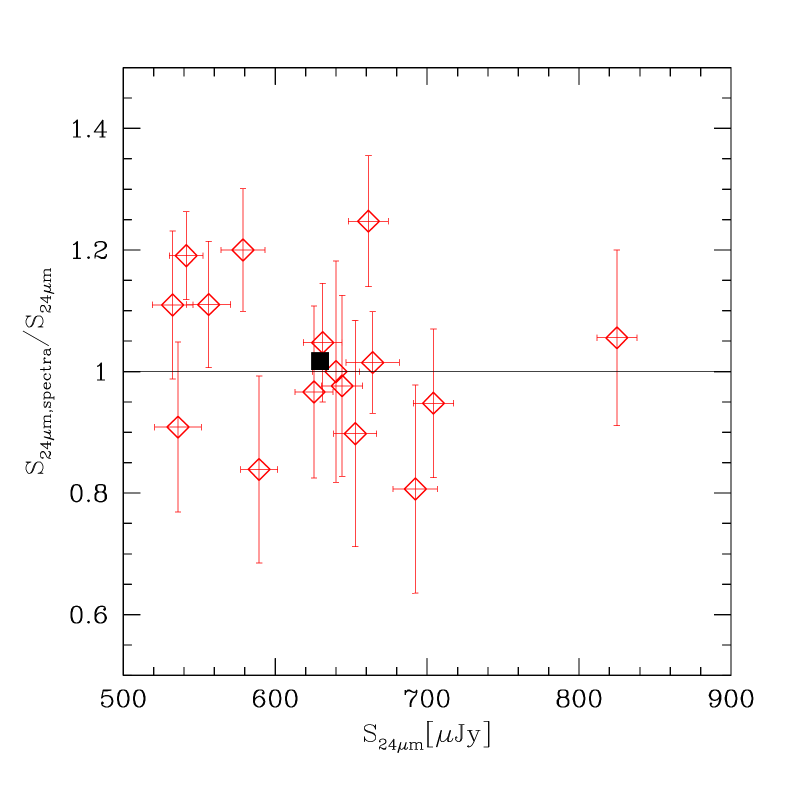
Figure 1: Ratio of $S_{\rm 24\,\mu m,spectra}$ deduced from our spectra using the MIPS 24 $\mu$m filter, to $S_{\rm 24\,\mu m}$ from the 2007 SWIRE internal catalogue, as a function of $S_{\rm 24\,\mu m}$. The black square is the mean for our full sample. The error bars correspond to 1 $\sigma$.

4.1 PAH redshifts

Applying the method described in Bertincourt et al. (2009), we have determined redshifts from PAH features ($z_{\rm PAH}$). This method is based on the cross-correlation of 21 templates with our IRS spectra. These templates are spectra of different kinds of sources. Five templates are dominated by PAHs (Smith et al. 2007). 13 are less PAH-dominated local ULIRGs from Armus et al. (2007), including among others Arp 220 and Mrk 231. The remaining three are a radio galaxy, a quasar, and a Wolf-Rayet galaxy. The best estimate of the redshift, $z_{\rm PAH}$, is the average of redshifts found for all templates after rejection in cases of very high $\chi^{2}$ ($\chi^{2}$/SNR $>8$) or too low SNR ($<1$). These redshifts are reported in Table 3. The estimated rms error of $z_{\rm PAH}$ is on average $\langle\Delta z_{\rm PAH}\rangle=0.010$ (median = 0.007; min = 0.004; max = 0.064). We also report in Table 3 the redshift, $z_{\rm best}$, of the best-matching template. The small differences between $z_{\rm PAH}$ and the redshift for the best-matching template are very consistent with the estimated rms error $\langle\Delta z_{\rm PAH}\rangle$. We use $z_{\rm PAH}$ in the following analysis because this determination is less biased by template selection than the redshift from the best-matching template ($\langle z_{\rm best}\rangle=2.011$; median = 1.994; scatter = 0.023). We note that $z_{\rm PAH}$ and $z_{\rm best}$ are very similar for all of our sample, and that our sources are best matched by a specific “PAH” template from Smith et al. (2007). The average of $z_{\rm PAH}$ is $2.017\pm 0.38$ (median = 1.997). The IRS redshifts of our sample span a narrower range, from 1.7 to 2.3, than the photometric redshifts maybe due to the strong $S_{\rm 24\,\mu m}$. This result is compatible with the fact that “5.8 $\mu$m-peakers” have a high probability of being dominated by a strong starburst at $z\sim 2$ because the stellar bump at 1.6 $\mu$m rest-frame is redshifted to around 5.8 $\mu$m at redshift $\sim 2$ (see, e.g., Lonsdale et al. 2009). Compared to the photometric redshifts reported in F09 found using the Hyper-z code (Bolzonella et al. 2000), the difference is fairly significant (see Fig. 2). Nevertheless, except for four sources, the photometric redshifts differ from $z_{\rm PAH}$ by less than 15%, the boundary for catastrophic outliers defined by Rowan-Robinson et al. (2008).

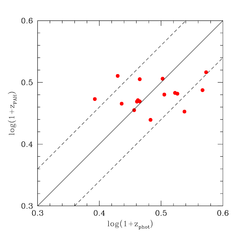
Figure 2: PAH spectroscopic redshift $z_{\rm PAH}$ as a function of photometric redshift from F09. The dashed lines correspond to $\Delta\,{\rm log}\,(1+z)=\pm 0.06$ or $\pm 15\%$.

4.2 Spectral decomposition

We perform spectral decompositions using the PAHFIT code developed by Smith et al. (2007). PAHFIT adjusts some PAH features and spectral lines as a function of rest wavelength (Fig. 3). The PAH features are represented by Drude profiles and the atomic and molecular spectral lines by Gaussians. The decomposition also tries to fit a stellar continuum component ($T_{\star}=5000\,{\rm K}$) and dust components for different temperatures (35, 50, 135, 200, 400, 600, 800, 1000, and 1200 K) represented by modified blackbodies. Only the intermediate dust temperatures make significant contributions to the mid-IR continuum. The dust extinction, mostly due to silicate absorption, is also taken into account. In our decompositions, we have adopted a screen geometry, corresponding to a uniform mask of dust absorbing the emission, to model the silicate absorption (Smith et al. 2007). Figure 3 presents an example of the result of the spectral decomposition. The PAH complexes at 6.2, 7.7, 8.6, and 11.3 $\mu$m are clearly visible. As proposed by Smith et al. (2007), the 7.7, 8.6, and 11.3 $\mu$m features are better fit by combinations of several features at 7.42, 7.60, and 7.85 $\mu$m for the 7.7 $\mu$m feature, at 8.33 and 8.61 $\mu$m for the 8.6 $\mu$m feature, and at 11.23 and 11.33 $\mu$m for the 11.3 $\mu$m feature. The results of our decompositions are somewhat uncertain, due to the difficulty of estimating the silicate absorption. However, this absorption is known to be weak to moderate in such starburst sources (e.g. Spoon et al. 2007; Farrah et al. 2008; Weedman & Houck 2008; Li & Draine 2001; Yan et al. 2005). Our targets appear to have especially weak absorption making them a good sample for analyzing with this decomposition approach. The spectral decompositions for the entire sample are reported in Appendix B for individual sources, and in Fig. 4 for the stacked spectrum of all 16 sources (see also Fig. 12). It is seen from individual spectra and the stack that the level of the continuum between 5 and 11 $\mu$m remains modest compared to the PAH features (except for L10, Sec. 6.1).

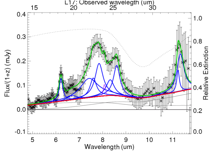
Figure 3: Spectral decomposition for source L17. The solid green line is the fitted model. Blue lines above the continuum are PAH features; violet lines are spectral lines. Thin grey lines represent thermal dust continuum components. The thick red line shows the total continuum (stars+dust). The dotted black line shows the extinction ($e^{-\tau_{\lambda}}$, $=1$ for no extinction). In this example, the top axis is labelled in observed wavelength. The redshift is $z_{\rm PAH}=1.959$. Spectral decompositions for the other sources are presented in Appendix B.

In the stacked spectrum (Fig. 4), a weak line is visible at $\sim$9.7 $\mu$m and identified as the 0-0 S(3) pure rotational transition of molecular hydrogen at 9.665 $\mu$m ($J=5-3$) in the PAHFIT spectral decomposition. This line is also visible in the partial stacks of Fig. 12 and may be present in the spectral decompositions of 13/16 sources (Fig. 16). The detection of this line is confirmed by the detailed data analysis that we perform in a separate paper (Fiolet et al. in prep.). The very large luminosity of this line, stronger than the CO luminosity, probably implies very strong shocks to excite its upper level $\sim$2500 K above the ground state of H₂, although ${\rm H_{2}}$ excitation could also be influenced by X-rays or UV from AGN. We also see hints of other lines, although not at significant levels: the S(5) and S(4) transitions of molecular hydrogen at $6.86\,{\rm\mu m}$ and $8.08\,{\rm\mu m}$, respectively, as well as the ionized species [Ar III] at $8.98\,{\rm\mu m}$ and [S IV] at $10.52\,{\rm\mu m}$.

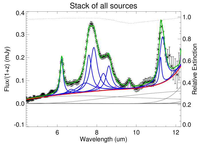
Figure 4: Spectral decomposition for the stacked spectrum of all 16 sources. The solid green line is the fitted model. The blue lines above the continuum are the PAH features. The narrow violet lines are the spectral lines. The grey lines represent the thermal dust continuum components. The thick red line shows the total continuum (stars+dust). The dotted black line shows the extinction ($e^{-\tau_{\lambda}}$, $=1$ if no extinction).

For each spectrum, we evaluate the continuum flux density and luminosity density at 5.8 $\mu$m ($\nu\,L_{\nu}$(5.8 $\mu$m)). These values are reported in Table 5. There is only a small dispersion of $\nu\,L_{\nu}$(5.8 $\mu$m) for our sources (average = $1.87\times 10^{11}\,L_{\odot}$, median = $1.77\times 10^{11}\,L_{\odot}$, min = $0.71\times 10^{11}\,L_{\odot}$, max = $2.99\times 10^{11}\,L_{\odot}$). In Fig. 5, we plot PAH luminosity at 7.7 $\mu$m ($L_{\rm 7.7\,\mu m}$) as a function of $\nu\,L_{\nu}$(5.8 $\mu$m). The PAH luminosity at 7.7 $\mu$m is calculated as the integral of the total flux between 7.3 $\mu$m and 7.9 $\mu$m after subtraction of the continuum contribution (see Eq. 1). We have also plotted the sample of Sajina et al. (2007). To make a true comparison, we have applied a similar reduction and spectral decomposition to the PAH-rich sources from Sajina et al. (2007). The values of $\nu\,L_{\nu}$(5.8 $\mu$m) found in this case show no significant difference from the published continuum luminosities. We see, in Fig. 5, that our sample shows somewhat weaker $\nu\,L_{\nu}$(5.8 $\mu$m) than the PAH-rich sample of Sajina et al. (2007) or the AGN-dominated sample of Coppin et al. (2010), while the values of $L_{\rm 7.7\,\mu m}$ stay in the same range. This is likely due to a stronger AGN contribution in the sample of Sajina et al. (2007). Note also that the ratio $L_{\rm 7.7\,\mu m}/\nu\,L_{\nu}$(5.8 $\mu$m) is very consistent with that found for the local starbursts of Brandl et al. (2006).

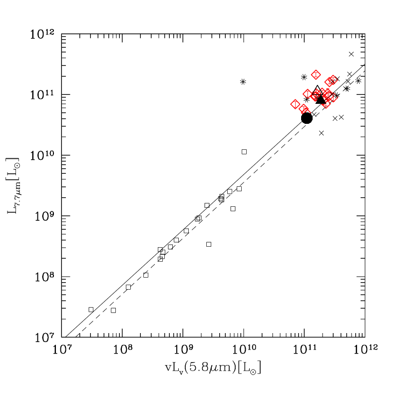
Figure 5: $L_{\rm 7.7\,\mu m}$ as a function of the continuum luminosity $\nu\,L_{\nu}$(5.8 $\mu$m). The red diamonds are the sources of our sample. The open (full) black triangle is the stack of our sources with EW${}_{\rm 7.7\,\mu m}>\,(<)\,6\,{\rm\mu m}$. The full black circle is the composite spectrum of the SMG sample from Menéndez-Delmestre et al. (2009). The black crosses are the PAH-rich sources from Sajina et al. (2007). The black asterisks are the AGN-dominated sources from Coppin et al. (2010). The black line is the best fit of all these samples. The dashed black line is the best fit to the local starbursts from Brandl et al. (2006) (black squares).

4.3 PAH features

Figure 6: $L_{\rm 7.7\,\mu m}$ as a function of $L_{\rm 6.2\,\mu m}$. The red diamonds are the sources of our sample. The open (full) black triangle is the stack of our subsample with EW${}_{\rm 7.7\,\mu m}>\leavevmode\nobreak\ (<)\leavevmode\nobreak\ 6\leavevmode\nobreak\ {\rm\mu m}$. The full black circle is the stacked spectrum of the SMG sample from Menéndez-Delmestre et al. (2009). The black circles are the intermediate-redshift star-forming galaxies from Shi et al. (2009). The black stars are the sample of SMGs from Pope et al. (2008). The black crosses are the PAH-rich sources from Sajina et al. (2007). The black asterisks are the AGN-dominated sources from Coppin et al. (2010). The full black squares are the sources from Farrah et al. (2008). The open black squares are the local star-forming galaxies from Brandl et al. (2006). The solid line is our best fit to all these samples. The dashed line is the best fit found by Pope et al. (2008) for their SMGs and the local starbursts.

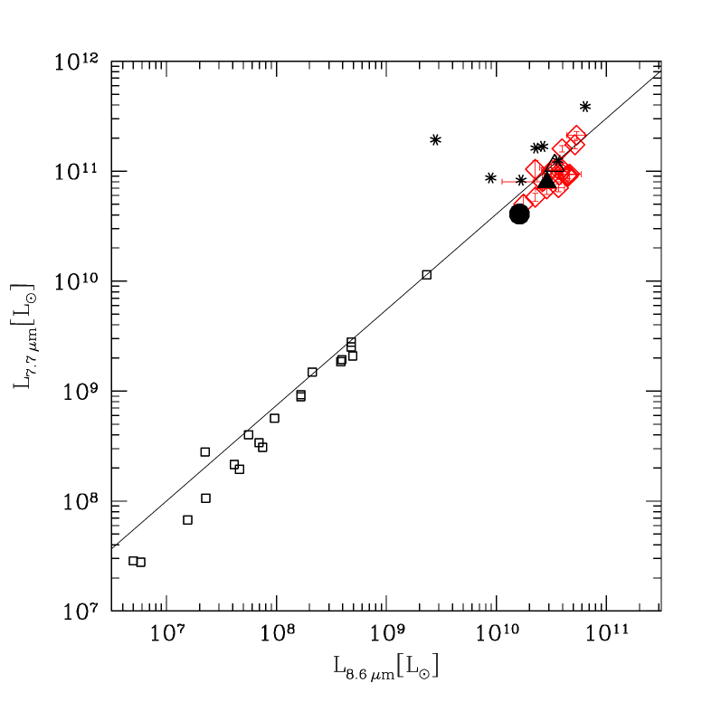
Figure 7: $L_{\rm 7.7\,\mu m}$ as a function of $L_{\rm 8.6\,\mu m}$. The symbols and the line are the same as in Fig. 6.

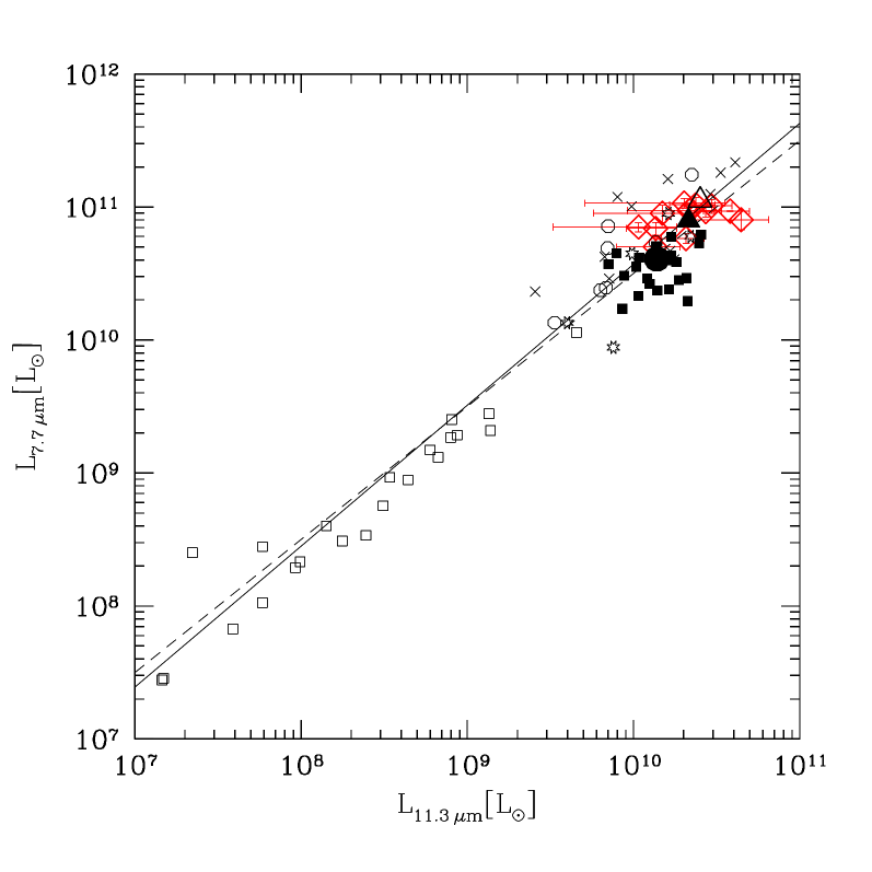
Figure 8: $L_{\rm 7.7\,\mu m}$ as a function of $L_{\rm 11.3\,\mu m}$. The symbols and the lines are the same as in Fig. 6.

Thanks to the spectral decomposition, we have determined the fluxes ($F$) and equivalent widths (EW) for the PAH complexes at 6.2, 7.7, 8.6, and 11.3 $\mu$m (Table 4). The flux is calculated by integrating the spectra between 6.2 and 6.3 $\mu$m, 7.3 and 7.9 $\mu$m, 8.3 and 8.7 $\mu$m, and 11.2 and 11.4 $\mu$m, respectively, after subtracting the continuum flux. We calculate the associated luminosities $L_{\rm 6.2\,\mu m}$, $L_{\rm 7.7\,\mu m}$, $L_{\rm 8.6\,\mu m}$, and $L_{\rm 11.3\,\mu m}$, reported in Table 5, using:

$$L_{i}=4\pi D_{L}^{2}F_{i}$$ (1)

where $D_{L}$ is the luminosity distance and $F_{i}=\int_{\lambda_{1}}^{\lambda_{2}}(S_{\lambda}-S_{c})d\lambda$ with $S_{\lambda}$ and $S_{c}$ the total and the continuum flux densities at the considered wavelengths.

The equivalent width is calculated following:

$$EW=\int_{\lambda_{1}}^{\lambda_{2}}\frac{S_{\lambda}-S_{c}}{S_{c}}d\lambda$$ (2)

All our sources show $L_{\rm 7.7\,\mu m}\ga 5\times 10^{10}\,L_{\odot}$ and EW${}_{\rm 7.7\,\mu m}>2\,\mu$m, i.e., well above the EW${}_{\rm 7.7\,\mu m}>0.8\,\mu$m limit for “strong” PAH sources defined by Sajina et al. (2007). All our sources except L10 also show EW${}_{\rm 6.2\,\mu m}\gg 0.2\,\mu$m and $L_{\rm 6.2\,\mu m}\gg 2\times 10^{10}\,L_{\odot}$. These values are usually used to separate starburst- from AGN-dominated sources (Armus et al. 2007).

Our sample has PAH luminosities on average comparable to those of the PAH-rich sources of Sajina et al. (2007) and slightly larger than those of the SMGs observed by Pope et al. (2008) and Menéndez-Delmestre et al. (2009), and of the “4.5 $\mu$m-peakers” of Farrah et al. (2008). Such a behavior might be naturally explained by stronger $S_{\rm 24\,\mu m}$ than SMG samples samples and higher redshift than Farrah et al. (2008)’s sample. The S/N of our average luminosities are higher than the other samples (Table 6). Indeed, the mean values of $L_{\rm 6.2\,\mu m}$, $L_{\rm 7.7\,\mu m}$, $L_{\rm 8.6\,\mu m}$, and $L_{\rm 11.3\,\mu m}$ are $2.90\pm 0.31$, $10.38\pm 1.09$, $3.62\pm 0.27$, and $2.29\pm 0.26\times 10^{10}\,L_{\odot}$, respectively, for our sample. The stated uncertainties are the standard deviations of the means. These values of luminosities are simple averages. The weighted averages and the measurements from the stacked spectra of our sources give luminosities consistent with the simple averages within the uncertainties. For example, the weighted average of $L_{\rm 6.2\,\mu m}$ is ($2.70\pm 0.09)\times 10^{10}\,L_{\odot}$, and the value derived from the stacked spectrum is ($2.81\pm 0.94)\times 10^{10}\,L_{\odot}$.

As seen in Figures 6, 7, and 8, and in Table 7, our PAH luminosities $L_{\rm 6.2\,\mu m}$, $L_{\rm 7.7\,\mu m}$, $L_{\rm 8.6\,\mu m}$, and $L_{\rm 11.3\,\mu m}$ have ratios similar to those of SMGs, as well as local starbursts and star-forming galaxies at $z\sim 1$. The AGN-dominated sample from Coppin et al. (2010) seems to have slightly different ratios, with a higher $L_{\rm 7.7\,\mu m}/L_{\rm 8.6\,\mu m}$.

The samples plotted in Figs. 6, 7, and 8 follow the relations

$$\rm{log}\,({\it L}_{\rm 7.7\,\mu m}) = (1.04\pm 0.03)\,\rm{log}\,({\it L}_{\rm 6.2\,\mu m})+(0.10\pm 0.32)$$ (3)

$$\rm{log}\,({\it L}_{\rm 7.7\,\mu m}) = (0.87\pm 0.04)\,\rm{log}\,({\it L}_{\rm 8.6\,\mu m})+(1.91\pm 0.34)$$ (4)

$$\rm{log}\,({\it L}_{\rm 7.7\,\mu m}) = (1.06\pm 0.03)\,\rm{log}\,({\it L}_{\rm 11.3\,\mu m})-(0.03\pm 0.30)$$ (5)

Note that these relations are just plain fits of the displayed samples of Figs. 6–8. As these samples may be biased in various ways, and the properties of the galaxies may vary with redshift, one should not expect a strong statistical consistency for these relations. The relations for $L_{\rm 6.2\,\mu m}$ and $L_{\rm 11.3\,\mu m}$ are consistent with the relations found by Pope et al. (2008) for local starbursts and SMGs.

These relations show that both $L_{\rm 7.7\,\mu m}/L_{\rm 6.2\,\mu m}$ and $L_{\rm 7.7\,\mu m}/L_{\rm 11.3\,\mu m}$ are $\sim 4$ for our sources at $z\sim 2$ (see also Figs. 13 and 14 and Table 7), i.e., about twice as large as for the local starbursts of Brandl et al. (2006) and the sources of Farrah et al. (2008) at $z\sim 1.7$. On the other hand, the ratio $L_{\rm 7.7\,\mu m}/L_{\rm 8.6\,\mu m}$ is about twice as small in these luminous galaxies at $z\sim 2$ as in fainter local starbursts (Table 7). This behavior is similar to that of SMGs (Table 7 and Sec. 6.2). The difference with respect to local starbursts could be explained by a difference in the size or ionization of PAH grains (Sec. 6.1, 6.2 and Fig. 14), or by a different extinction due to silicates around 10 $\mu$m (affecting the 8.6 and 11.3  $\mu$m bands) or ice at $\sim$6 $\mu$m (absorbing the 6.2 $\mu$m band) (Menéndez-Delmestre et al. 2009; Spoon et al. 2002). However, the effects of extinction seem somewhat contradictory for the different band ratios. The finding of a lower 7.7/8.6 ratio compared to normal, local starbursts, is consistent with a low silicate extinction in our sample, as does the generally low level of extinction in the spectral fits. However, the ’larger’ 7.7/11.3 ratio that we report is going in the other direction; similarly, our ’larger’ 7.7/6.2 ratio would imply a larger ice absorption than in local starbursts.

L10 is the only source that seems not to follow the relation between $L_{\rm 7.7\,\mu m}$ and $L_{\rm 6.2\,\mu m}$, showing too weak a feature at 6.2 $\mu$m. However, Table 5 and Fig. 6 show that the deviation of L10 from the correlation remains within the statistical errors of this noisy spectrum. The offset is probably due to higher extinction or a more energetically important AGN (Rigopoulou et al. 1999); see also Sec. 6.1.

4.4 Silicate absorption

The determination of the optical depth of the silicate absorption at 9.7 $\mu$m ($\tau_{9.7}$), reported in Table 4, is a product of the general fit of the spectra with PAHFIT. It is based on interstellar extinction similar to that of the Milky Way (Smith et al. 2007). We note that the silicate absorption is weak on average, $\langle\tau_{9.7}\rangle=0.28$ (0.50 if we consider only the sources with $\tau_{9.7}\neq 0$) vs. 1.09 for the PAH-rich sample of Sajina et al. (2007). Indeed, for 44% (7/16) of our sources, PAHFIT provides $\tau_{9.7}=0$. It is clear that all values of extinction ($\tau_{9.7}$) are very uncertain because of the weakness of the continuum and its uncertainty, and because of the lack of measurements at long wavelengths. We thus state only the qualitative conclusion that the average extinction is likely weak in most of our sources. Considering the values of EW_6.2 and $\tau_{9.7}$, most of our sources belong to class 1C of the diagram of Spoon et al. (2007, their Figs. 1 & 3). This class is defined by spectra dominated by PAH emission with weak silicate absorption.

5 PAH emission and star formation

As noted above, it is well known that infrared PAH emission is strongly correlated with star formation through excitation and IR fluorescence of PAHs induced by the UV radiation of young stars. The exceptional quality of our PAH spectra at $z\sim 2$ allows us to further assess the correlation between PAH luminosity and total IR luminosity, and to compare with other starburst samples at $z\sim 2$ and at lower redshift. The deep radio data allow a precise comparison with the radio luminosity which is also known to trace the starburst IR luminosity well.

5.1 The correlation between IR and PAH luminosities

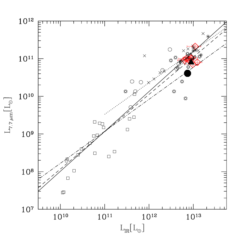
Figure 9: $L_{\rm 7.7\,\mu m}$ as a function of $L_{\rm IR}$. The symbols are the same as in Fig. 6. The solid line is our best fit to all samples. The dashed line is the best fit found by Pope et al. (2008) from fitting both their SMGs and the local starbursts. The dotted line is the best fit found by Shi et al. (2009). The dot-dashed line is the best fit found by Menéndez-Delmestre et al. (2009).

The correlation between the strength of the PAH emission and the far-IR luminosity in starbursts is well established although not understood in detail. Remarkably, it has been verified among local starburst galaxies over two orders of magnitude in $L_{\rm IR}$, from 10¹⁰ to 10${}^{12}\,L_{\odot}$, by Brandl et al. (2006). The approximate proportionality between $L_{\rm 7.7\,\mu m}$ and $L_{\rm IR}$ has been extended through the ULIRG range up to 10${}^{13}\,L_{\odot}$ and $z\geq 2$ by several studies (Shi et al. 2009; Pope et al. 2008; Menéndez-Delmestre et al. 2009). Our sample gives us an opportunity to check how tight the relation is among the strongest starbursts at $z\sim 2$.

For the nine sources of our sample observed at 350 $\mu$m by Kovács et al. (2010) – all SMGs (F09) – we have an accurate estimate of the infrared luminosity $L_{\rm IR}$ computed by Kovács et al. (2010), who fit a distribution of grey-body models with different dust temperatures (multi-temperature model). All these sources are powerful ULIRGs with $L_{\rm IR}$ close to 10${}^{13}\,L_{\odot}$ (average = $8.87\times 10^{12}\,L_{\odot}$, $\langle\Delta L_{\rm IR}\rangle=2.81\times 10^{12}\,L_{\odot}$; see Table 5). The average value of the ratio of IR and PAH luminosities is

$$\langle L_{\rm 7.7\,\mu m}/L_{\rm IR}\rangle=11.7\times 10^{-3}$$ (6)

It is seen in Table 7 and Fig. 9 that the $L_{\rm 7.7\,\mu m}/L_{\rm IR}$ ratio is within a factor $\sim 2$ of those for the other high-$z$ samples. However, it is a factor $\sim 3.5$ larger than for less luminous local starbursts as yielded by Eq. 6. Schweitzer et al. (2006) have also demonstrated the existence of a correlation between the strength of the PAH emission and the far-IR luminosity for local starburst-dominated ULIRGs and QSO hosts. Nevertheless, the $\langle L_{\rm 7.7\,\mu m}/L_{\rm IR}\rangle$ ratio that they found is probably lower because of the more compact nature of those objects.

In Fig. 9, we plot $L_{\rm 7.7\,\mu m}$ as a function of $L_{\rm IR}$ for different samples. We can see that our sample has $L_{\rm IR}$ comparable to those of the other SMG samples (Pope et al. 2008; Menéndez-Delmestre et al. 2009), and the PAH-rich sources from Sajina et al. (2007). The star-forming galaxies of Shi et al. (2009) have $L_{\rm IR}$ values slightly lower than our sample. We also note that the best fit of all these samples is consistent with the relations found by Pope et al. (2008) and Menéndez-Delmestre et al. (2009) for SMGs and local starbursts (Brandl et al. 2006). The AGN-dominated sample of Coppin et al. (2010) shows $L_{\rm IR}$ and $L_{\rm 7.7\,\mu m}$ greater than our sources, but their ratio is not very different from our sample. The sources of Shi et al. (2009) seem to follow a slightly different relation but with the same slope as the fit found by Menéndez-Delmestre et al. (2009). The best fit of all these samples, from local starbursts to SMGs, is

$${\rm log}\,(L_{\rm 7.7\,\mu m})=(1.06\pm 0.04)\,{\rm log}\,(L_{\rm IR})-(2.57\pm 0.52)\\$$ (7)

This relation is consistent with $L_{\rm 7.7\,\mu m}$ being a good tracer of high-z starbursts: a strong $L_{\rm 7.7\,\mu m}$ should be the sign of a high SFR. If we use our relation between $L_{\rm 7.7\,\mu m}$ and $L_{\rm IR}$ and assume the relation from Kennicutt (1998) between SFR and $L_{\rm IR}$ based on a 0.1–100 $M_{\odot}$ Salpeter-like IMF, we obtain the following relation

$${\rm log}\,({\rm SFR})=0.94\,{\rm log}\,(L_{\rm 7.7\,\mu m})-7.27$$ (8)

where SFR is in units of $M_{\odot}$ yr^-1.

This relation is slightly different from that found by Menéndez-Delmestre et al. (2009). The latter is based on the luminosity at 7.7 $\mu$m calculated from the total flux between 7.1 $\mu$m and 8.3 $\mu$m after continuum substraction, instead of between 7.3 $\mu$m and 7.9 $\mu$m as in our case. However, the values of $L_{\rm 7.7\,\mu m}$ computed with the two definitions are very comparable. Applying Eq. 8, we find on average $\langle{\rm SFR}\rangle=1260\pm 470\,M_{\odot}$ yr^-1. This value is consistent with the average SFR of 1060 M_⊙ yr^-1 computed from the radio luminosity in F09, and close to the median SFR of $\sim$ 1200 M_⊙ yr^-1 found for SMGs by Menéndez-Delmestre et al. (2009).

5.2 The correlation between 1.4 GHz and PAH luminosities

The correlation between radio luminosity ($L_{\rm 1.4\,GHz}$) and far-infrared luminosity in star-forming regions and in local starbursts is well known (e.g., Helou et al. 1985; Condon 1992; Crawford et al. 1996; Sanders & Mirabel 1996). This correlation has been confirmed at $z\sim 2$ by Chapman et al. (2005) (see also F09; Condon 1992; Smail et al. 2002; Yun & Carilli 2002; Ivison et al. 2002; Kovács et al. 2006; Sajina et al. 2008; Younger et al. 2009; Ivison et al. 2010; Magnelli et al. 2010).

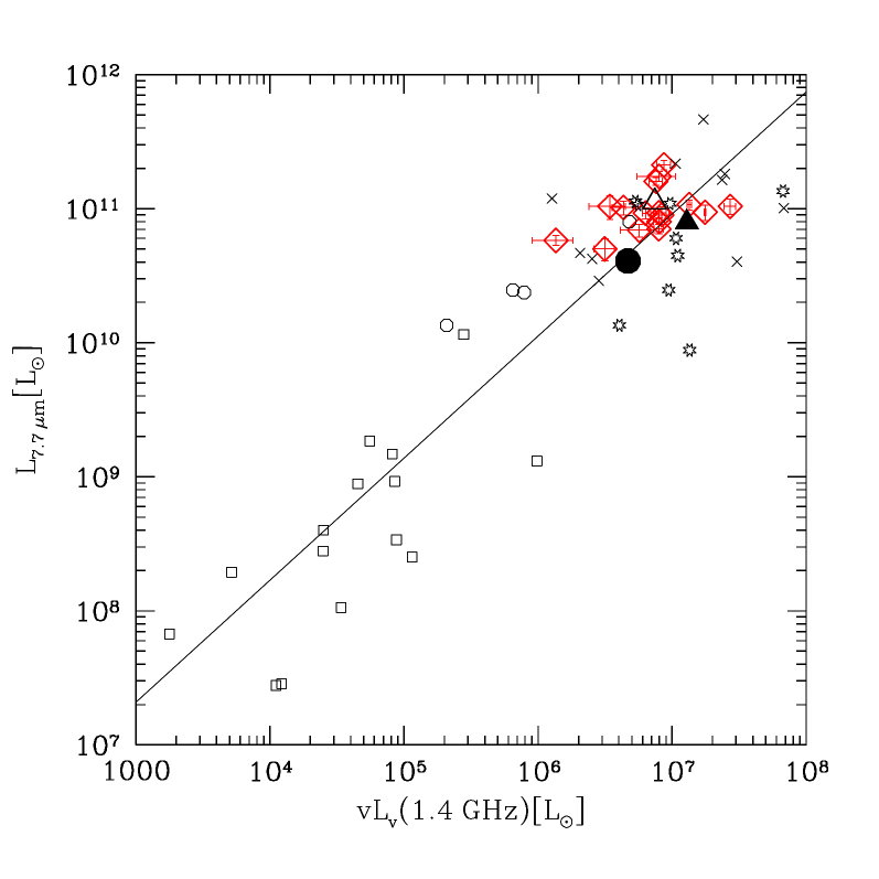
Figure 10: $L_{\rm 7.7\,\mu m}$ as a function of rest-frame $\nu\,L_{\nu}$(1.4 GHz). The symbols are the same as in Fig. 6. The black line is our best fit to all these samples.

From the correlation between $L_{\rm IR}$ and $L_{\rm 7.7\,\mu m}$ (Fig. 9, Eq. 7), we might expect a very good correlation between PAH and radio luminosities, as previously observed by Pope et al. (2008). Since our sources benefit from exceptionally good radio data at 20 cm, 50 cm, and 90 cm (Sec. 2.1), it is worthwhile to directly check the tightness of this relation.

It is straightforward to compute the rest-frame luminosity at 1.4 GHz ($L_{\rm 1.4\,GHz}=\nu\,L_{\nu}$(1.4 GHz)) using, e.g., the formula given by Kovács et al. (2006):

$$\nu\,L_{\nu}({\rm 1.4\,GHz})=4\pi D_{L}^{2}\,S_{\rm 20\,cm}\,(1.4\times 10^{9})\,(1+z)^{(-\alpha-1)}$$ (9)

where $D_{L}$ is the luminosity distance and $\alpha$ is the radio spectral index defined by the best power law fit, $S_{\nu}\propto\nu^{\alpha}$, between $S_{\rm{20\,cm}}$, $S_{\rm{50\,cm}}$, and $S_{\rm{90\,cm}}$. We have computed $\nu\,L_{\nu}$(1.4 GHz) for our sample and those of Sajina et al. (2007), Pope et al. (2008), Shi et al. (2009), and Brandl et al. (2006). For our sample, we have used $\alpha$ as computed in F09 and reported in Table 1. For the PAH-rich sample of Sajina et al. (2007), we have used the values published in Sajina et al. (2008). For the other samples, we use the average value of $\alpha$, $\langle\alpha\rangle=-0.64$ found in F09, which is consistent with the typical radio spectral index for star-forming galaxies (e.g., Condon 1992). The values of $\nu\,L_{\nu}$(1.4 GHz) are reported in Table 5.

As expected, we observe a correlation between $L_{\rm 1.4\,GHz}$ and $L_{\rm 7.7\,\mu m}$. Considering our sample, but also the local star-forming galaxy sample (Brandl et al. 2006), the sample of SMGs (Pope et al. 2008), the PAH-rich sources from Sajina et al. (2007), and the intermediate-redshift starbursts (Shi et al. 2009), we obtain the following relation (Fig 10):

$${\rm log}\,(L_{\rm 7.7\,\mu m})=(0.91\pm 0.06)\,{\rm log}\,(L_{\nu}(\rm 1.4\,GHz))+(4.60\pm 0.36)$$ (10)

The effect of the positive $k$-correction and the value of $\alpha$ are particularly important for the determination of $L_{\rm 1.4\,GHz}$ and may significantly affect the reliability of the relation stated in Eq. 10. The correlation between $L_{\rm 1.4\,GHz}$ and $L_{\rm 7.7\,\mu m}$ seems to be more scattered than the correlation between $L_{\rm IR}$ and $L_{\rm 7.7\,\mu m}$. It is not surprising considering the uncertainties on $L_{\rm 1.4\,GHz}$ and the scatter of the correlation between $L_{\rm IR}$ and $L_{\rm 1.4\,GHz}$ as shown by e.g. Kovács et al. (2010).

5.3 PAH emission and stellar mass

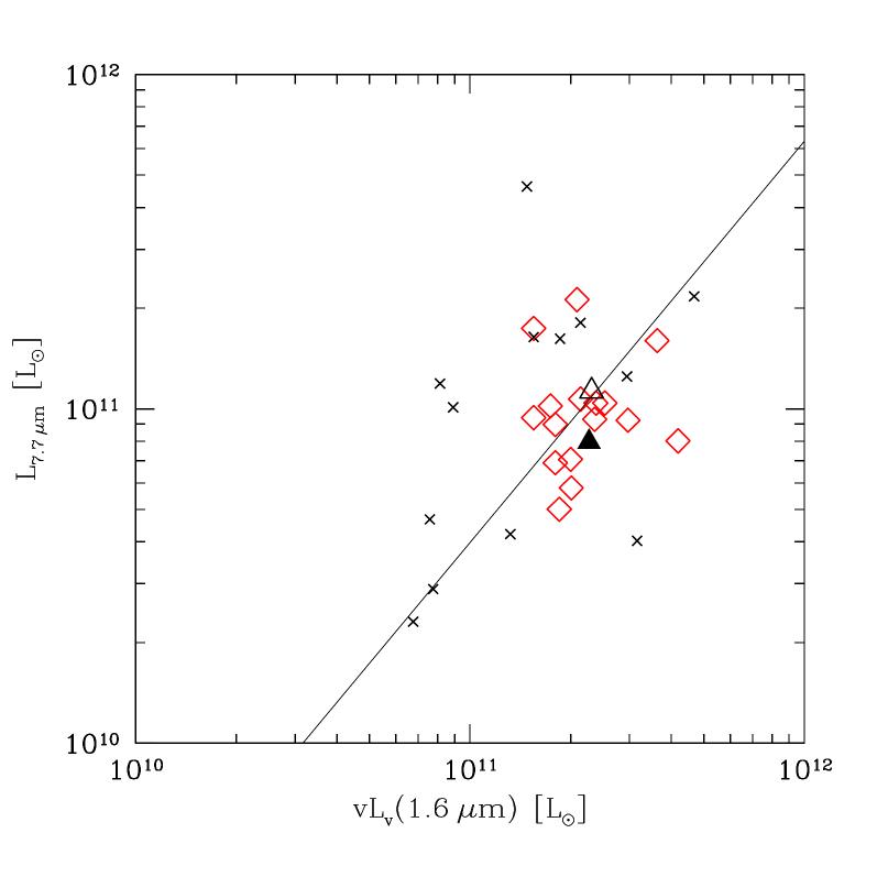
Figure 11: $L_{\rm 7.7\,\mu m}$ as a function of the stellar bump luminosity $L_{\rm 1.6\,\mu m}$. The symbols are the same as in Fig. 6. Only the samples at $z\sim 2$ are plotted. The line is the best fit found for the “normal” star-forming galaxies of Lu et al. (2003).

The stellar bump luminosity at 1.6 $\mu$m ($\nu\,L_{\nu}$(1.6 $\mu$m), reported in Table 5, gives an estimate of the stellar mass ($M_{\star}$) of our sources (see, e.g., F09; Seymour et al. 2007; Lonsdale et al. 2009). Applying the same mass-to-light ratio as F09 ($M_{\star}/\nu\,L_{\nu}({\rm 1.6\,\mu m})=0.7\,M_{\odot}/L_{\odot}$), $M_{\star}$ derived from $\nu\,L_{\nu}$(1.6 $\mu$m) ranges from 1.1 to $3.0\times 10^{11}\,M_{\odot}$ (average = 1.6$\times$10${}^{11}\,M_{\odot}$, median = 1.4$\times$10${}^{11}\,M_{\odot}$).

In Fig. 11, we plot $L_{\rm 7.7\,\mu m}$ as a function of $\nu\,L_{\nu}$(1.6 $\mu$m) for our sources and the PAH-rich sample from Sajina et al. (2007). Our sample shows no clear difference from the sources of Sajina et al. (2007) in terms of $\nu\,L_{\nu}$(1.6 $\mu$m). Both samples follow the relation found for “normal” star-forming galaxies (Sajina et al. 2007; Lu et al. 2003). This result implies that $L_{\rm 7.7\,\mu m}$ and $\nu\,L_{\nu}$(1.6 $\mu$m) do not trace AGN (Sajina et al. 2007). Since the PAH luminosity is tightly correlated with the star formation rate, the relation between $\nu\,L_{\nu}$(1.6 $\mu$m) and $L_{\rm 7.7\,\mu m}$ seems to confirm the existence of a correlation between star formation rate and stellar mass at $z\sim 2$ as previously observed by Pannella et al. (2009) and Mobasher et al. (2009). However, note that the mass-to-light ratio remains uncertain because of uncertainty in the age of the dominant stellar population.

6 Discussion

6.1 Distinction between starburst and AGN

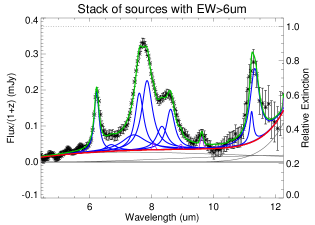
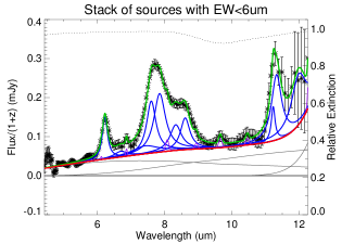
Figure 12: PAHFIT spectral decomposition of stacked spectra. Upper panel: 7 sources with EW${}_{\rm 7.7\,\mu m}>6\,\mu$m. Lower panel: 9 sources with EW${}_{\rm 7.7\,\mu m}<6\,\mu$m. The solid green line is the fitted model. The blue lines above the continuum are the PAH features. The narrow violet lines are the spectral lines. The grey lines represent the thermal dust continuum components. The thick red line shows the total continuum (stars+dust). The dotted black line shows the extinction ($e^{-\tau_{\lambda}}$  $=1$ if no extinction).

As previously discussed, the relative strength of the PAH features and the mid-IR continuum is a very efficient criterion for distinguishing starburst- from AGN-dominated ULIRGs (e.g., Yan et al. 2007; Sajina et al. 2007; Weedman et al. 2006; Houck et al. 2005). Genzel et al. (1998) and Rigopoulou et al. (1999) use the parameter 7.7 $\mu$m-(L/C), defined as the ratio between the peak flux density at 7.7 $\mu$m and the continuum flux density at the same wavelength, to distinguish between AGN and starburst. AGN-dominated composite sources show values of 7.7 $\mu$m-(L/C) weaker than starburst-dominated systems. An equivalent straightforward indicator is the equivalent width of the PAH features, especially EW${}_{\rm 7.7\,\mu m}$, since it is proportional to the ratio of $L_{\rm 7.7\,\mu m}$ to the 7.7 $\mu$m continuum. The equivalent widths of our sources span a broad range, more than a factor of 5. Despite the large uncertainty in the continuum, e.g., as estimated by PAHFIT, it is clear that EW${}_{\rm 7.7\,\mu m}$ should be a relevant parameter for discussion of AGN contributions. For our entire sample, we find $\langle{\rm EW}_{\rm 7.7\,\mu m}\rangle=5.64\,{\rm\mu m}$ (median = 4.88) vs. 3.04 $\mu$m for the stacked spectrum of Menéndez-Delmestre et al. (2009).

Based on the values of EW${}_{\rm 7.7\,\mu m}$ (see Table 4), we have constructed two subsamples: the first has EW${}_{\rm 7.7\,\mu m}>6\,\mu$m (7 sources, $\langle{\rm EW}_{\rm 7.7\,\mu m}\rangle=8.33\,\mu$m) and the second has EW${}_{\rm 7.7\,\mu m}<6\,\mu$m (9 sources, $\langle{\rm EW}_{\rm 7.7\,\mu m}\rangle=3.55\,\mu$m). We have produced stacked spectra of these two subsamples, built from the weighted means of the individual spectra scaled to $\langle F_{\rm 7.7\,\mu m}\rangle$. They are plotted in Fig. 12. It is obvious, as expected, that the second subsample has a significantly stronger continuum.

Applying the same method as Menéndez-Delmestre et al. (2009), we estimate an X-ray luminosity ($L_{X}$) from the 10 $\mu$m continuum flux (Table 4) via the Krabbe et al. (2001) relation. Then assuming the $L_{X}/L_{\rm IR}$ found for AGN by Alexander et al. (2005), we estimate the contribution of AGN to $L_{\rm IR}$. We find that the AGN contribution is $\sim 20\%$ for our whole sample and $\sim 10\%$ and $\sim 25\%$ for the subsamples with EW${}_{\rm 7.7\,\mu m}>6\,\mu$m and with EW${}_{\rm 7.7\,\mu m}<6\,\mu$m, respectively. Menéndez-Delmestre et al. (2009) have found $\sim 32\%$ to be the AGN contribution in SMGs. The difference can be interpreted as a difference in the continuum flux density, with continuum larger by a factor $\sim 2$ for the sample of Menéndez-Delmestre et al. (2009).

In Fig. 9 (see also Table 6), it is seen that the two subsamples are not different in term of $L_{\rm IR}$ and follow the correlation between $L_{\rm 7.7\,\mu m}$ and $L_{\rm IR}$ found in Sec. 5.1. This result tends to argue that the majority of the IR luminosity is associated with the starburst and not with the AGN. This is not the case in the sample of Menéndez-Delmestre et al. (2009), which shows a smaller $L_{\rm 7.7\,\mu m}/L_{\rm IR}$ ratio, implying that the AGN contributes more to $L_{\rm IR}$ (Table 7).

Another possible sign of a strong AGN contribution is a large $L_{\rm 7.7\,\mu m}/L_{\rm 6.2\,\mu m}$ ratio, as discussed by, e.g., Rigopoulou et al. (1999) and Pope et al. (2008). They have observed such a rise in $L_{\rm 7.7\,\mu m}$ versus $L_{\rm 6.2\,\mu m}$ for some SMGs, which they attribute to greater silicate absorption in the presence of a more luminous AGN than is seen in most SMGs or starburst galaxies. Stronger silicate absorption significantly affects $L_{\rm 8.6\,\mu m}$ and $L_{\rm 11.3\,\mu m}$, while it may lead to an overestimate of $L_{\rm 7.7\,\mu m}$. However, as seen in Figs. 6 and 8, there is no significant difference in the value of $L_{\rm 7.7\,\mu m}/L_{\rm 6.2\,\mu m}$ between sources with large and small EWs, perhaps because the silicate absorption is small.

We see in Fig. 10 and Table 6 that sources with EW${}_{\rm 7.7\,\mu m}<6\,\mu$m seem to have an average value of $\nu\,L_{\nu}$(1.4 GHz) somewhat greater than that of sources with EW${}_{\rm 7.7\,\mu m}>6\,\mu$m. Radio excess could be a good indication of AGN strength (Seymour et al. 2008; Archibald et al. 2001; Reuland et al. 2004). However, we note that practically all of this difference is due to two sources in the small-EW subsample, L11 and L17, which are close to the radio loudness limit at $z\sim 2$ as defined by Jiang et al. (2007) and Sajina et al. (2008): $\nu$ L${}_{\nu}({\rm 1.4\,GHz})=3.66\times 10^{7}\,L_{\odot}$. They are thus good candidates for having significant AGN emission. Applying the same method as previously to determinate the AGN contribution, we find 26% and 19% for L11 and L17, respectively.

To summarize: although small, it seems that the AGN contribution is slightly greater in the sources with EW${}_{\rm 7.7\,\mu m}<6\,\mu$m than the systems with EW${}_{\rm 7.7\,\mu m}>6\,\mu$m. Nevertheless, all these sources show strong PAH emission and individually follow more or less the relations found for local starbursts (Brandl et al. 2006). They are probably all starburst-dominated or AGN-starburst composite sources, with at most a weak AGN contribution to the mid-infrared.

Our sample is particularly homogeneous in term of PAH luminosity (see Table 5). Only one source, L10, is different. Indeed, this source shows a spectrum slightly different from the others. Its continuum is stronger and has a larger slope (Fig. 16). Moreover, L10 deviates from the correlation between $L_{\rm 6.2\,\mu m}$ and $L_{\rm 7.7\,\mu m}$ with a low $L_{\rm 6.2\,\mu m}$. L10 also presents the weakest EW${}_{\rm 6.2\,\mu m}$, EW${}_{\rm 7.7\,\mu m}$, and EW${}_{\rm 8.6\,\mu m}$ of our sample, with values of 0.10, 2.32, and 0.77 $\mu$m, respectively. Such a difference can be explained by a larger AGN contribution to the mid-infrared emission, and also by a low signal-to-noise ratio (see Fig 15). Nevertheless, the fact that L10 follows the other correlations – especially the correlation between $\nu\,L_{\nu}$(1.4 GHz) and $L_{\rm 7.7\,\mu m}$ – seems to prove that this source is starburst-dominated. The same kind of source was observed by Pope et al. (2008).

6.2 Comparison with other studies

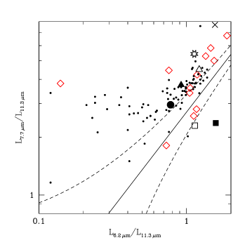
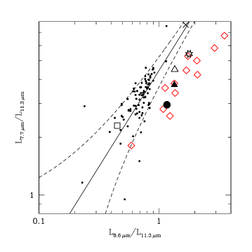
Figure 13: Upper panel: $L_{\rm 7.7\,\mu m}/L_{\rm 11.3\,\mu m}$ as a function of $L_{\rm 6.2\,\mu m}/L_{\rm 11.3\,\mu m}$. Lower panel: $L_{\rm 7.7\,\mu m}/L_{\rm 11.3\,\mu m}$ as a function of $L_{\rm 8.6\,\mu m}/L_{\rm 11.3\,\mu m}$. In both panels, the red diamonds are the sources in our sample. The small black circles are the sample of O’Dowd et al. (2009). The open (full) black triangle is the stack of our sources with EW${}_{\rm 7.7\,\mu m}>\,(<)\,6\,\mu$m. The black cross shows the average for the PAH-rich sources from Sajina et al. (2007). The black star shows the average for the sample of SMGs from Pope et al. (2008). The open black square shows the average for the local star-forming galaxies from Brandl et al. (2006). The full black square is the average for the sample of “4.5 $\mu$m-peakers” from Farrah et al. (2008). The large black circle is based on the composite spectrum of the SMG sample from Menéndez-Delmestre et al. (2009). The black line and the dotted lines are the best linear regression and the $1\sigma$ dispersion found by Galliano et al. (2008) for Galactic HII regions, dwarf spirals, and starburst galaxies.

The present work is based on a complete sample of 16 sources selected to be starburst “5.8 $\mu$m-peakers” that are bright at 24 $\mu$m, with $S_{\rm 24\,\mu m}>0.50$ mJy. The average flux density of our sample is $\langle S_{\rm 24\,\mu m}\rangle=0.63$ mJy. This is a brighter sample of SMGs compared to that of Pope et al. (2008) ($\langle S_{\rm 24\,\mu m}\rangle=0.45$ mJy) or Menéndez-Delmestre et al. (2009) ($\langle S_{\rm 24\,\mu m}\rangle=0.33$ mJy). On the other hand, the PAH-rich sample of Sajina et al. (2007) is biased toward the brightest $24\,{\rm\mu m}$ sources, with a mean $\langle S_{\rm 24\,\mu m}\rangle=1.19$ mJy. Our sample is also brighter than the ULIRGs at $z\sim 2$ of Fadda et al. (2010) ($\langle S_{\rm 24\,\mu m}\rangle=0.27$ mJy). All these samples have an average redshift $z\sim 2$, but ours spans a narrower redshift range than the others. Indeed, our sample has $z_{\rm PAH}$ between 1.75 and 2.28, while the samples of Pope et al. (2008) and Menéndez-Delmestre et al. (2009), the ULIRGs from Fadda et al. (2010) and the PAH-rich sample of Sajina et al. (2007) span $z=0.93-2.55$, 0.69–3.62, 1.62–2.44, and 0.82–2.47, respectively.

The differences between PAH luminosities for all the samples are small, but our PAH luminosities show an higher S/N than the other high-redshift samples (Table 6). Our sample has PAH luminosities in all bands quite comparable to those of Sajina et al. (2007) and about twice as large as those of Pope et al. (2008) and Menéndez-Delmestre et al. (2009).

As regards the PAH-band luminosity ratios, we see in Table 7 that our sample is not very different in term of ratios from the other SMG samples (Pope et al. 2008; Menéndez-Delmestre et al. 2009; Sajina et al. 2007). Nevertheless, Menéndez-Delmestre et al. (2009) find lower ratios for $L_{\rm 6.2\,\mu m}/L_{\rm IR}$ and $L_{\rm 7.7\,\mu m}/L_{\rm IR}$. This is probably due to a greater AGN contribution to $L_{\rm IR}$ (Sec. 6.1).

Our sample also shows a higher $L_{\rm 7.7\,\mu m}/L_{\rm IR}$ ratio than the lower-redshift sample of Brandl et al. (2006). This difference could be explained by a more extended PAH distribution in our sources. Indeed, if the PAH distribution is extended, a larger fraction of PAH can survive in strong UV radiation field from AGN or young stars. Then $L_{\rm 7.7\,\mu m}/L_{\rm IR}$ becomes higher than in compact PAH distributions where PAH are easier destroyed by UV radiation field (e.g., Huang et al. 2009).

In Fig. 13, we plot the different PAH ratios of these samples following O’Dowd et al. (2009). We find that our sample and the other SMG samples show $L_{\rm 7.7\,\mu m}/L_{\rm 11.3\,\mu m}$ vs. $L_{\rm 6.2\,\mu m}/L_{\rm 11.3\,\mu m}$ ratios consistent with the sample of O’Dowd et al. (2009). The sample of Brandl et al. (2006) falls in the border of the dispersion for the PAH ratios of Galactic HII regions, dwarf spirals, and starburst galaxies found by Galliano et al. (2008). The plot of $L_{\rm 7.7\,\mu m}/L_{\rm 11.3\,\mu m}$ vs. $L_{\rm 8.6\,\mu m}/L_{\rm 11.3\,\mu m}$ shows that all these samples have ratios different from those of O’Dowd et al. (2009) because of stronger emission at 8.6 $\mu$m. Our sample does not follow the relation found by Galliano et al. (2008).

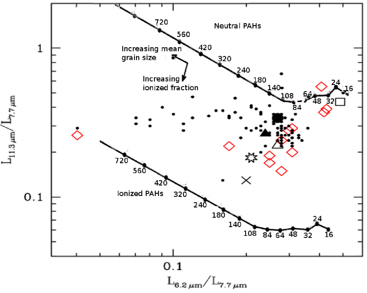
Figure 14: Adapted from O’Dowd et al. (2009): $L_{\rm 11.3\,\mu m}/L_{\rm 7.7\,\mu m}$ as a function of $L_{\rm 6.2\,\mu m}/L_{\rm 7.7\,\mu m}$. The symbols are the same as in Fig. 13. The black lines represent the expected ratios for fully neutral or fully ionized PAH molecules of a given number of carbon atoms from the models of Draine & Li (2001).

A likely explanation of these differences in PAH ratios is modification of the size or ionization of PAH grains. Fig. 14, adapted from O’Dowd et al. (2009), seems to prove that our sample has PAH grains with sizes comparable to those in the other samples of SMGs, but with a slightly lower fraction of ionized grains than the samples of Pope et al. (2008) and (especially) Sajina et al. (2007). Brandl et al. (2006) find smaller and more neutral grains in local starbursts than our sample. The difference could arise due to the strongest ionizing UV radiation from young stars in the most powerful starbursts but less ionising than in the sample of Pope et al. (2008) and Menéndez-Delmestre et al. (2009) probably because of lower AGN contamination.

7 Summary and conclusions

In this paper, we have presented the results of Spitzer/IRS observations of a complete sample of 16 sources selected to be 24 $\mu$m-bright and “5.8 $\mu$m-peakers.” The spectra obtained show very strong PAH features at 6.2, 7.7, 8.6, and 11.3 $\mu$m, along with a weak continuum. Thanks to these exceptionally strong features, we have estimated accurate PAH redshifts that span the range $z=1.75-2.28$. Our average PAH redshift is $\langle z_{\rm PAH}\rangle=2.02\pm 0.15$, and the average error of the individual $z_{\rm PAH}$ is $\langle\Delta z_{\rm PAH}\rangle=0.010$ (median = 0.007; min = 0.004; max = 0.064). The stacked spectrum of our 16 sources displays evidence for the pure rotational 0-0 S(3) molecular hydrogen line at $\lambda=9.67\,\mu$m, which is confirmed and analyzed in a separate paper.

Thanks to the very good quality of our IRS spectra, we have calculated PAH luminosities $L_{\rm 6.2\,\mu m}$, $L_{\rm 7.7\,\mu m}$, $L_{\rm 8.6\,\mu m}$, and $L_{\rm 11.3\,\mu m}$ to have average values $2.90\pm 0.31$, $10.38\pm 1.09$, $3.62\pm 0.27$, and $2.29\pm 0.26\times 10^{10}\,L_{\odot}$, respectively. These luminosities have a S/N higher than the other SMGs samples. We have studied the correlation between $L_{\rm 7.7\,\mu m}$ and the other PAH luminosities. All our sources, except perhaps L10, follow a correlation similar to that found for local starbursts, and they are not very different from other samples of SMGs at $z\sim 2$. We have also confirmed the very good correlation, previously observed, between $L_{\rm 7.7\,\mu m}$ and $L_{\rm IR}$ at high redshift, and we have verified its extension to the radio luminosity $\nu\,L_{\nu}$(1.4 GHz). It also extends more loosely to stellar mass through $\nu\,L_{\nu}$(1.6 $\mu$m).

All these relations, the luminosity ratios, and the equivalent widths allow us to estimate the AGN contribution to the mid-IR luminosity. We conclude that our sources are starburst-dominated and that the AGN contribution is $\sim$20%. This sample is the most pure selection of massive starbursts at $z\sim 2$ compared to the other $z\sim 2$ Spitzer-selected samples. The known fact that the equivalent width of PAH features is a good discriminant between starburst-dominated and AGN-dominated sources is reinforced by the study of two subsamples of sources with EW${}_{\rm 7.7\,\mu m}\,>6\,\mu$m and EW${}_{\rm 7.7\,\mu m}<6\,\mu$m. The subsample with EW${}_{\rm 7.7\,\mu m}<6\,\mu$m shows a larger AGN contribution ($\sim 25\%$) than the EW${}_{\rm 7.7\,\mu m}>6\,\mu$m subsample ($\sim 10\%$), although the AGN contribution is small in both subsamples.

Appendix A Spectra and best fit-templates

In Fig. 15, we present our spectra and the best-fit templates among the 21 templates described in Sec 4.1 using the method described in Bertincourt et al. (2009). We also plot the 24 $\mu$m flux densities from the SWIRE catalogue and the values determined from the IRS spectra convolved with the MIPS 24 $\mu$m filter.

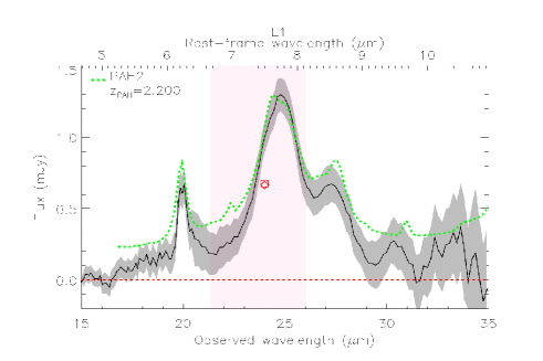
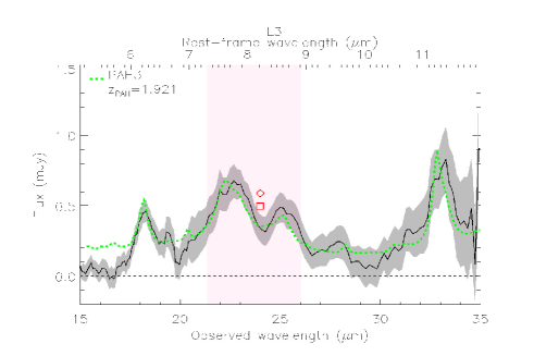
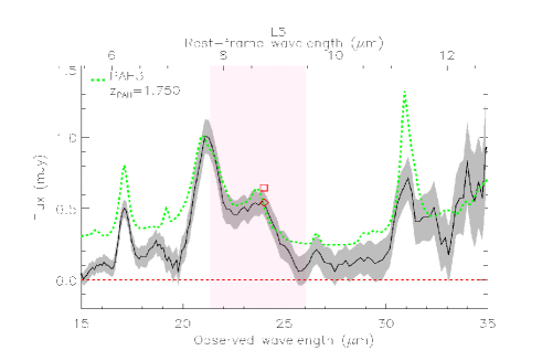
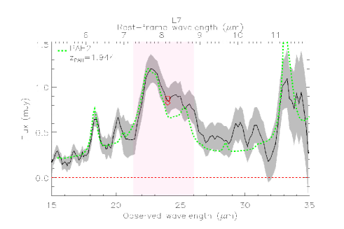
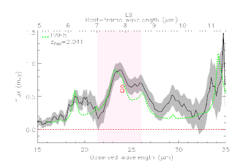
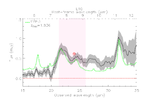
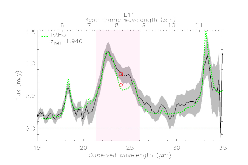
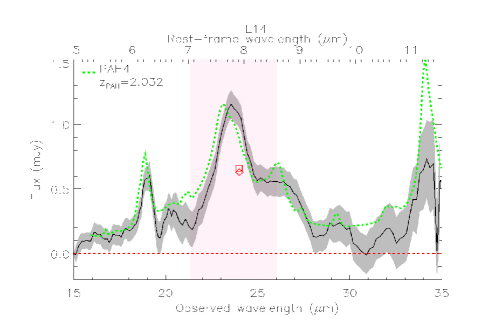
Figure 15: IRS spectra of our sources. The black line is our data. In shaded grey, we plot the 1$\sigma$ deviation. The green short-dashed line is the best-fit PAH template from Smith et al. (2007). The red diamond is the 24 $\mu$m flux density from the SWIRE catalogue. The red square is the 24 $\mu$m flux density extracted from the spectrum with the 24 $\mu$m filter profile. The pink shape shows the region where the transmission of the 24 $\mu$m is maximum. All these spectra are plotted in observed wavelength. The templates are scaled to the ”$(1+z)\times 7.7\,\mu$m” flux. The source ID, the names of the best-fit templates, and $z_{\rm PAH}$ are reported in each panel.

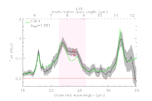
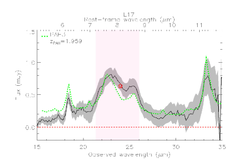
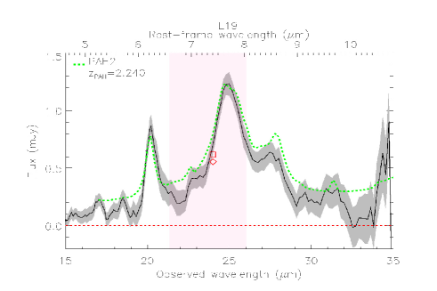
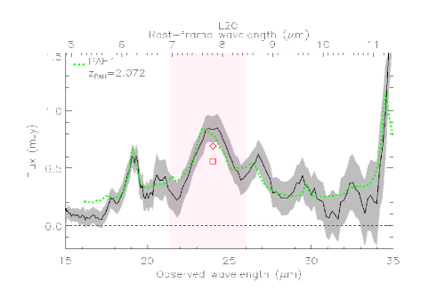
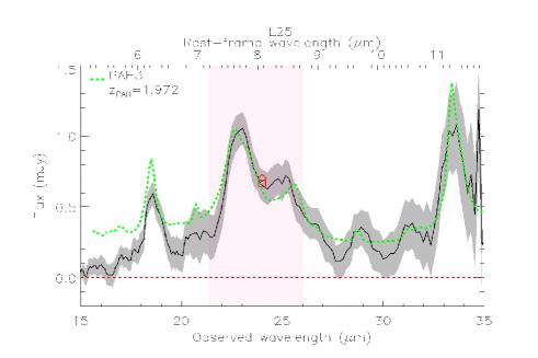
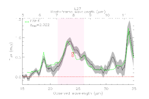
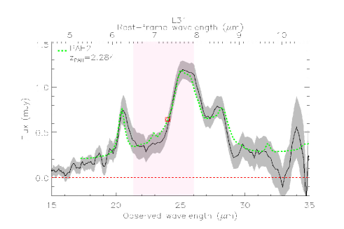
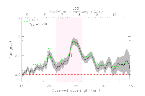
Figure 15: Continued

Appendix B Spectral decomposition of the spectra

In Fig. 16, we present the decompositions of our spectra made with the PAHFIT code developed by Smith et al. (2007).

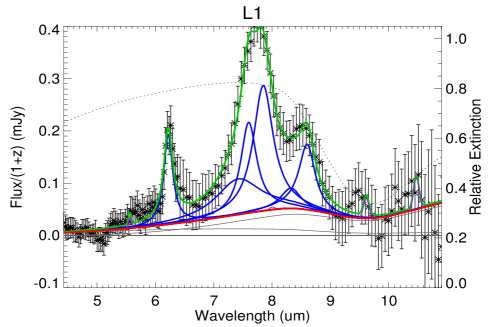
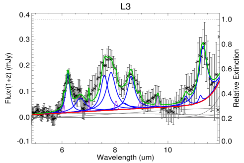
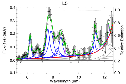
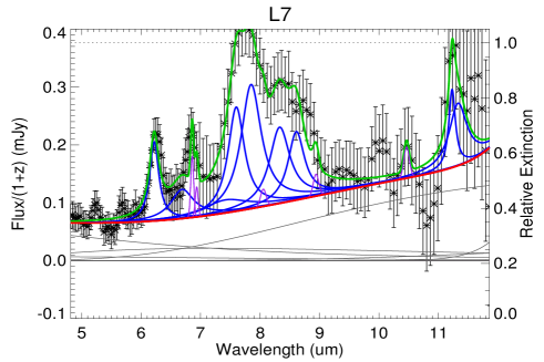
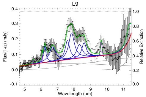
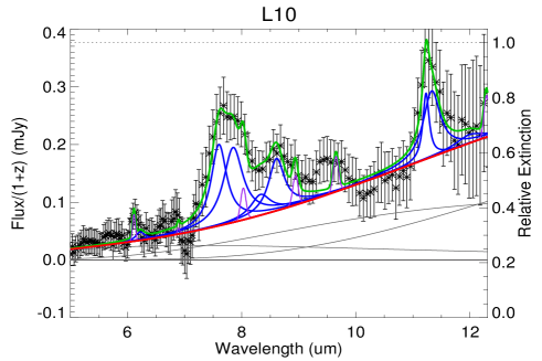
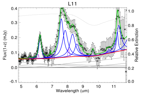
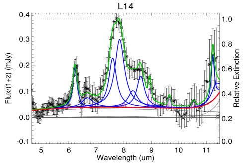
Figure 16: Decompositions of the spectra of our sources. The solid green line is the fitted model. The blue lines above the continuum are the PAH features. The violet lines are the spectral lines. The thin grey lines represent the thermal dust continuum components. The thick red line shows the total continuum (stars+dust). The dotted black line shows the extinction ($e^{-\tau_{\lambda}}$, $=1$ if no extinction). The source ID is reported as the title of each panel.

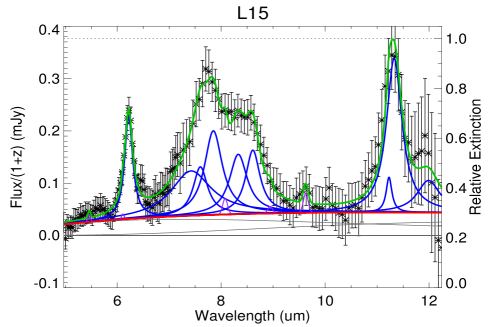
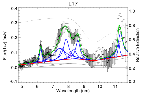
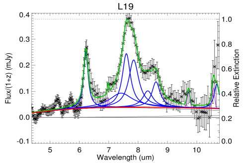
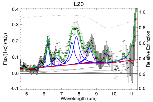
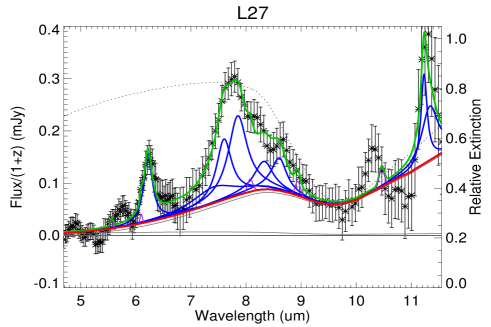
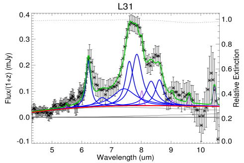
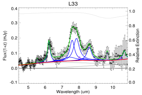
Figure 16: Continued

Table 1: Spitzer mid-IR, submillimeter, and radio data of the selected sample.

IDa	IAU name	$S_{\rm{24\,\mu m}}$b	$S_{\rm 24\,\mu m,spectra}$c	$S_{\rm{350\,\mu m}}$d	$S_{\rm{1.2\,mm}}$a	$S_{\rm{20\,cm}}$e	$\alpha$f
		($\mu$Jy)		(mJy)		($\mu$Jy)
L1	SWIRE4_J104351.17+590058.1	664$\pm$18	674$\pm$38	30.0$\pm$10.5	2.95$\pm$0.66	76.3$\pm$9.0	-0.84
L3	SWIRE4_J104410.00+584056.0	589$\pm$12	495$\pm$80	$\mathellipsis$	1.04$\pm$1.11	105.5$\pm$35.0	+0.86
L5	SWIRE4_J104427.52+584309.6	542$\pm$11	645$\pm$26	$\mathellipsis$	2.75$\pm$0.76	71.0$\pm$20.0	-1.03
L7	SWIRE4_J104430.60+585518.6	825$\pm$13	871$\pm$105	$\mathellipsis$	1.39$\pm$0.79	101.7$\pm$13.3	-0.81
L9	SWIRE4_J104440.25+585928.3	653$\pm$14	586$\pm$109	55.1$\pm$17.1	4.00$\pm$0.55	116.5$\pm$9.2	-0.54
L10	SWIRE4_J104549.77+591904.0	626$\pm$12	605$\pm$76	$\mathellipsis$	1.39$\pm$0.81	67.2$\pm$11.7	-0.40
L11	SWIRE4_J104556.90+585318.8	661$\pm$13	825$\pm$55	38.9$\pm$5.8	3.08$\pm$0.58	314.8$\pm$4.1	-0.45
L14	SWIRE4_J104638.68+585612.5	631$\pm$13	661$\pm$48	29.7$\pm$4.9	2.13$\pm$0.71	159.5$\pm$6.0	-0.73
L15	SWIRE4_J104656.46+590235.5	579$\pm$14	695$\pm$41	25.7$\pm$5.9	2.36$\pm$0.62	68.6$\pm$3.7	-1.03
L17	SWIRE4_J104704.97+592332.3	644$\pm$14	629$\pm$83	45.3$\pm$12.4	2.24$\pm$0.64	341.0$\pm$33.0	-0.76
L19	SWIRE4_J104708.78+590627.2	556$\pm$14	618$\pm$42	$\mathellipsis$	0.89$\pm$0.97	102.2$\pm$12.0	-0.44
L20	SWIRE4_J104717.96+590231.7	692$\pm$15	558$\pm$107	51.6$\pm$7.2	2.66$\pm$0.78	51.1$\pm$4.7	-1.25
L25	SWIRE4_J104738.32+591010.0	704$\pm$13	667$\pm$74	36.1$\pm$7.1	2.56$\pm$0.74	69.0$\pm$9.0	-1.09
L27	SWIRE4_J104744.60+591413.5	533$\pm$13	591$\pm$50	27.4$\pm$7.9	2.48$\pm$0.73	77.2$\pm$13.7	-0.38
L31	SWIRE4_J104830.70+585659.3	640$\pm$16	640$\pm$101	$\mathellipsis$	1.62$\pm$0.60	121.0$\pm$39.0	-0.31
L33	SWIRE4_J104848.23+585059.3	536$\pm$15	487$\pm$61	$\mathellipsis$	-0.28$\pm$1.09	109.0$\pm$33.0	+0.27

^aIDs and $S_{\rm{1.2\,mm}}$ are the same as F09. The bold values are $>$3 $\sigma$ detections

^b$S_{\rm{24\,\mu m}}$ comes from the internal SWIRE catalogue.

^c$S_{\rm 24\,\mu m,spectra}$ is calculated by convolution of the 24 $\mu$m MIPS filter and our spectra.

^d$S_{\rm{350\,\mu m}}$ comes from Kovács et al. (2010).

^e$S_{\rm{20\,cm}}$ comes from Owen & Morrison (2008).

^fThe radio spectral index $\alpha$ is calculated using the best power law fit, $S_{\nu}\propto\nu^{\alpha}$, between $S_{\rm{20\,cm}}$, $S_{\rm{50\,cm}}$, and $S_{\rm{90\,cm}}$ as reported in F09.

Table 2: Summary of Spitzer IRS observations.

ID	LL1 time on target	LL2 time on target
	(sec)
L7	2$\times$120$\times$6	8$\times$120$\times$6
L1, L9, L11, L17, L20, L25	3$\times$120$\times$6	8$\times$120$\times$6
L3, L10, L14, L15, L31	4$\times$120$\times$6	9$\times$120$\times$6
L5, L19, L27, L33	5$\times$120$\times$6	11$\times$120$\times$6

Table 3: Redshifts.

ID	$z_{\rm PAH}$a	$z_{\rm best}$b	mid-IR best matching template
			from Smith et al. (2007)
L1	2.200$\pm$0.005	2.196	pah2
L3	1.921$\pm$0.005	1.922	pah3
L5	1.750$\pm$0.007	1.756	pah3
L7	1.944$\pm$0.064	1.886	pah2
L9	2.041$\pm$0.007	2.046	pah5
L10	1.836$\pm$0.005	1.834	pah3
L11	1.946$\pm$0.010	1.946	pah5
L14	2.032$\pm$0.005	2.034	pah4
L15	1.851$\pm$0.010	1.844	pah4
L17	1.959$\pm$0.004	1.964	pah3
L19	2.240$\pm$0.012	2.222	pah2
L20	2.072$\pm$0.010	2.066	pah1
L25	1.972$\pm$0.005	1.974	pah3
L27	2.022$\pm$0.008	2.014	pah4
L31	2.284$\pm$0.009	2.272	pah2
L33	2.206$\pm$0.010	2.200	pah3

^aAverage PAH spectroscopic redshift.

^bRedshift for best-matching template.

Table 4: Fluxes and equivalent widths for PAH features from PAHFIT (Smith et al. 2007).

ID	$F_{\rm 6.2\,\mu m}$	$F_{\rm 7.7\,\mu m}$	$F_{\rm 8.6\,\mu m}$	$F_{\rm 11.3\,\mu m}$	EW${}_{\rm 6.2\,\mu m}$	EW${}_{\rm 7.7\,\mu m}$	EW${}_{\rm 8.6\,\mu m}$	EW${}_{\rm 11.3\,\mu m}$	$\tau_{9.7}$	$S_{\rm 10\,\mu m}$a
	(10-22 W.cm${}^{-2})$				($\mu$m)					(mJy)
L1	4.93$\pm$0.51	21.69$\pm$1.80	5.48$\pm$1.03	$\mathellipsis$	2.86	9.42	2.70	$\mathellipsis$	1.08	0.037
L3	3.44$\pm$0.51	8.28$\pm$0.69	3.22$\pm$1.30	2.94$\pm$0.85	2.90	8.17	2.67	1.85	0.00	0.036
L5	3.82$\pm$0.51	12.41$\pm$1.37	5.16$\pm$1.07	2.48$\pm$0.83	3.67	12.02	4.99	1.63	0.02	0.033
L7	3.11$\pm$0.56	12.44$\pm$1.82	6.22$\pm$2.24	2.13$\pm$1.26	0.55	2.82	1.37	0.52	0.00	0.133
L9	2.41$\pm$0.38	8.68$\pm$0.67	4.53$\pm$0.61	1.28$\pm$0.91	0.63	2.41	1.33	0.27	0.00	0.096
L10	0.29$\pm$0.50	7.99$\pm$1.51	2.83$\pm$1.33	2.10$\pm$0.89	0.10	2.32	0.77	0.48	0.00	0.128
L11	3.61$\pm$0.48	12.99$\pm$1.74	6.43$\pm$1.70	3.06$\pm$1.68	0.81	4.72	2.28	1.15	0.10	0.080
L14	3.37$\pm$0.57	13.17$\pm$1.10	4.39$\pm$1.30	2.50$\pm$1.87	1.19	7.54	2.80	3.17	0.00	0.034
L15	4.47$\pm$0.33	14.48$\pm$1.30	5.83$\pm$0.52	4.25$\pm$0.53	1.73	6.88	3.22	3.92	0.00	0.044
L17	2.38$\pm$0.51	14.10$\pm$1.82	5.39$\pm$0.75	3.16$\pm$0.96	0.84	5.04	2.21	1.71	0.54	0.051
L19	4.93$\pm$0.35	15.67$\pm$1.01	3.87$\pm$0.48	$\mathellipsis$	1.71	7.52	2.30	$\mathellipsis$	0.00	0.035
L20	3.85$\pm$0.63	9.49$\pm$1.49	3.11$\pm$1.77	5.25$\pm$2.46	1.31	4.40	1.30	2.83	0.18	0.066
L25	5.39$\pm$0.50	12.45$\pm$1.00	5.98$\pm$1.08	4.82$\pm$1.51	1.72	2.86	1.57	1.43	1.32	0.067
L27	3.77$\pm$0.42	12.77$\pm$1.54	3.40$\pm$0.77	3.54$\pm$1.18	1.81	3.43	1.12	1.01	1.09	0.069
L31	4.07$\pm$0.52	16.25$\pm$1.37	4.82$\pm$0.60	$\mathellipsis$	1.26	6.80	2.44	$\mathellipsis$	0.03	0.043
L33	3.12$\pm$0.41	10.57$\pm$2.11	2.29$\pm$0.86	$\mathellipsis$	0.93	3.93	1.01	$\mathellipsis$	0.10	0.054

^a$S_{\rm 10\,\mu m}$ is the continuum flux density at 10 $\mu$m.

Table 5: Luminosities for different wavelengths.

ID	$\nu\,L_{\nu}$(1.6 $\mu$m)a	$\nu\,L_{\nu}$(5.8 $\mu$m)	$L_{\rm 6.2\,\mu m}$	$L_{\rm 7.7\,\mu m}$	$L_{\rm 8.6\,\mu m}$	$L_{\rm 11.3\,\mu m}$	$\nu\,L_{\nu}$(1.4 GHz)a	$L_{\rm IR}$b
	(10${}^{11}\,L_{\odot}$)		(10${}^{10}\,L_{\odot}$)				(10${}^{6}\,L_{\odot}$)	(10${}^{12}\,L_{\odot}$)
L1	2.09	1.55	4.83$\pm$0.50	21.24$\pm$1.76	5.36$\pm$1.01	$\mathellipsis$	8.71$\pm$1.00	11.00$\pm$3.80
L3	2.01	0.97	2.41$\pm$0.35	7.80$\pm$5.12	2.26$\pm$0.91	2.07$\pm$0.59	1.35$\pm$0.43	$\mathellipsis$
L5	1.80	0.71	2.12$\pm$0.29	6.90$\pm$0.76	2.87$\pm$0.60	1.38$\pm$0.46	5.75$\pm$1.59	$\mathellipsis$
L7	1.80	2.99	2.24$\pm$0.40	9.73$\pm$7.18	4.49$\pm$1.62	1.54$\pm$0.91	8.32$\pm$1.15	$\mathellipsis$
L9	2.00	2.27	1.96$\pm$0.31	7.06$\pm$0.55	3.68$\pm$0.50	1.04$\pm$0.74	7.94$\pm$0.55	9.77$\pm$3.37
L10	1.85	1.06	0.18$\pm$0.31	5.01$\pm$0.95	1.77$\pm$0.83	1.32$\pm$0.56	3.16$\pm$0.58	$\mathellipsis$
L11	1.55	2.54	2.61$\pm$0.34	10.77$\pm$4.42	4.65$\pm$1.23	2.22$\pm$1.21	17.78$\pm$0.41	8.13$\pm$2.24
L14	2.14	1.96	2.72$\pm$0.46	11.63$\pm$5.30	3.54$\pm$1.05	2.02$\pm$1.51	13.49$\pm$0.62	8.51$\pm$2.54
L15	2.97	1.50	2.86$\pm$0.21	9.25$\pm$0.83	3.73$\pm$0.34	2.72$\pm$0.34	6.31$\pm$0.29	6.31$\pm$1.89
L17	2.38	1.57	1.76$\pm$0.38	10.37$\pm$1.34	3.96$\pm$0.55	2.33$\pm$0.71	26.92$\pm$2.48	9.12$\pm$3.36
L19	3.63	2.59	5.05$\pm$0.35	16.04$\pm$1.04	3.96$\pm$0.49	$\mathellipsis$	7.59$\pm$0.87	$\mathellipsis$
L20	4.19	2.05	3.25$\pm$0.53	9.82$\pm$5.96	2.63$\pm$1.50	4.43$\pm$2.08	7.94$\pm$0.73	12.30$\pm$3.40
L25	2.36	1.54	4.03$\pm$0.37	9.30$\pm$0.75	4.47$\pm$0.81	3.60$\pm$1.13	7.94$\pm$1.10	7.76$\pm$2.50
L27	1.74	1.13	3.00$\pm$0.34	10.16$\pm$1.22	3.18$\pm$0.61	2.82$\pm$0.94	4.37$\pm$0.80	6.92$\pm$2.23
L31	1.55	2.97	4.37$\pm$0.56	17.44$\pm$1.47	5.18$\pm$0.64	$\mathellipsis$	7.94$\pm$2.56	$\mathellipsis$
L33	2.53	2.43	3.08$\pm$0.40	10.42$\pm$2.08	2.26$\pm$0.85	$\mathellipsis$	3.39$\pm$1.01	$\mathellipsis$

^aFrom F09.

^bFrom Kovács et al. (2010).

Table 6: Average luminosities for different samples.

Sample	$\langle$z$\rangle$	$\langle S_{\rm 24\,\mu m}\rangle$	$L_{\rm 6.2\,\mu m}$	$L_{\rm 7.7\,\mu m}$	$L_{\rm 8.6\,\mu m}$	$L_{\rm 11.3\,\mu m}$	$\nu\,L_{\nu}$(1.4 GHz)	$L_{\rm IR}$
		(mJy)	(10${}^{10}\,L_{\odot}$)				(10${}^{6}\,L_{\odot}$)	(10${}^{12}\,L_{\odot}$)
This work	2.017	0.63	2.90$\pm$0.31	10.38$\pm$1.09	3.62$\pm$0.27	2.29$\pm$0.26	8.68$\pm$1.56	8.87$\pm$0.64
This work, EW7.7μm$>$6 $\mu$ma	2.040	0.60	3.07$\pm$0.13	11.30$\pm$0.35	3.42$\pm$0.15	2.51$\pm$0.29	7.31$\pm$1.38	8.61$\pm$1.35
This work, EW7.7μm$<$6 $\mu$ma	2.000	0.65	1.94$\pm$0.14	7.96$\pm$0.72	2.86$\pm$0.21	2.12$\pm$0.29	9.75$\pm$2.59	9.00$\pm$0.78
Sajina et al. (2007)b	1.524	1.19	2.66$\pm$0.46	13.17$\pm$3.28	2.87$\pm$0.67	1.71$\pm$0.37	18.33$\pm$6.50	6.32$\pm$1.36
Menédez-D. et al. (2009)c	2.000	0.33	1.09$\pm$0.22	4.10$\pm$0.93	1.63$\pm$0.17	1.39$\pm$0.10	4.63$\pm$0.79	7.37$\pm$2.45
Pope et al. (2008)	1.910	0.45	1.34$\pm$0.22	6.46$\pm$1.30	2.13$\pm$0.38	1.19$\pm$0.32	14.32$\pm$5.96	5.90$\pm$1.00
Coppin et al. (2010)	2.730	0.51	3.04$\pm$0.71	16.28$\pm$3.52	2.55$\pm$0.72	$\mathellipsis$	$\mathellipsis$	10.98$\pm$1.88
Farrah et al. (2008)	1.690	0.73	2.37$\pm$0.18	3.56$\pm$0.24	$\mathellipsis$	1.50$\pm$0.10	$\mathellipsis$	$\mathellipsis$
		(mJy)	(10${}^{8}\,L_{\odot}$)				(10${}^{5}\,L_{\odot}$)	(10${}^{11}\,L_{\odot}$)
Brandl et al. (2006)	0.008	8.52$\times$103	2.10$\pm$0.85	4.26$\pm$1.61	0.83$\pm$0.34	1.85$\pm$0.65	1.23$\pm$0.64	1.18$\pm$0.31
O’Dowd et al. (2009)	0.092	6.08	4.24$\pm$0.49	17.72$\pm$1.72	3.82$\pm$0.36	5.16$\pm$0.43	$\mathellipsis$	$\mathellipsis$

^aThe values are computed from the stacked spectra.

^aThe sample of Sajina et al. (2007) is limited to PAH-rich sources with EW${}_{\rm 7.7\mu m}>0.8\,\mu$m.

^bMenédez-D. et al. (2009) designates Menéndez-Delmestre et al. (2009).

Table 7: Average luminosities ratios for different samples.

Sample	$\frac{L_{\rm 6.2\,\mu m}}{L_{\rm 7.7\,\mu m}}$	$\frac{L_{\rm 6.2\,\mu m}}{L_{\rm 11.3\,\mu m}}$	$\frac{L_{\rm 7.7\,\mu m}}{L_{\rm 8.6\,\mu m}}$	$\frac{L_{\rm 7.7\,\mu m}}{L_{\rm 11.3\,\mu m}}$	$\frac{L_{\rm 8.6\,\mu m}}{L_{\rm 11.3\,\mu m}}$	$\frac{L_{\rm 6.2\,\mu m}}{L_{\rm IR}}$	$\frac{L_{\rm 7.7\,\mu m}}{L_{\rm IR}}$	$\frac{L_{\rm 7.7\,\mu m}}{\nu L_{\nu}({\rm 1.4\,GHz})}$
						(10-3)		(103)
This work	0.28	1.27	2.87	4.53	1.58	3.27	11.70	11.96
This work, EW${}_{\rm 7.7\mu m}>6\,\mu$ma	0.27	1.22	3.30	4.50	1.36	3.57	13.12	15.46
This work, EW${}_{\rm 7.7\mu m}<6\,\mu$ma	0.24	0.92	2.78	3.75	1.35	2.16	8.84	8.16
Sajina et al. (2007)b	0.20	1.56	4.59	7.70	1.68	4.21	20.84	7.18
Menéndez-Delmestre et al. (2009)	0.27	0.78	2.52	2.95	1.17	1.48	5.56	8.86
Pope et al. (2008)	0.21	1.13	3.03	5.43	1.79	2.27	10.95	4.51
Coppin et al. (2010)	0.19	$\mathellipsis$	6.38	$\mathellipsis$	$\mathellipsis$	2.77	14.83	$\mathellipsis$
Farrah et al. (2008)	0.66	1.58	$\mathellipsis$	2.37	$\mathellipsis$	$\mathellipsis$	$\mathellipsis$	$\mathellipsis$
Brandl et al. (2006)	0.49	1.14	5.13	2.30	0.45	1.77	3.61	3.46
O’Dowd et al. (2009)	0.24	0.83	4.63	3.44	0.74	$\mathellipsis$	$\mathellipsis$

^aThe values are computed from the stacked spectra.

^bThe sample of Sajina et al. (2007) is limited to PAH-rich sources with EW${}_{\rm 7.7\mu m}>0.8\,\mu$m.