Image formation in synthetic aperture radio telescopes

Abstract

Next generation radio telescopes will be much larger, more sensitive, have much larger observation bandwidth and will be capable of pointing multiple beams simultaneously. Obtaining the sensitivity, resolution and dynamic range supported by the receivers requires the development of new signal processing techniques for array and atmospheric calibration as well as new imaging techniques that are both more accurate and computationally efficient since data volumes will be much larger. This paper provides a tutorial overview of existing image formation techniques and outlines some of the future directions needed for information extraction from future radio telescopes. We describe the imaging process from measurement equation until deconvolution, both as a Fourier inversion problem and as an array processing estimation problem. The latter formulation enables the development of more advanced techniques based on state of the art array processing. We demonstrate the techniques on simulated and measured radio telescope data.

I Introduction

The field of radio astronomy is a relatively young field of observational astronomy, dating back to pioneering research by Jansky in the 1930s [1] who demonstrated that radio waves are emitted from the Milky Way galaxy. Inspired by his work, Reber [2] made the first radio survey of the sky using a radio telescope that he built in his backyard. Figure 1 depicts some results of his radio survey, including the strong radio emissions of Cygnus A (Cyg A) and Cassiopeia A (Cas A).

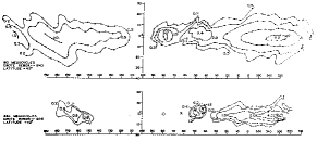
Figure 1: Reber’s radio survey. We can see the Milky way Galaxy, Cygnus A and Cassiopeia A. Image courtesy of NRAO/AUI

In 1946 Ryle and Vonberg [3] used the Michelson interferometer to observe radio emissions from the sun at a frequency of 175 MHz. Ryle continued to construct interferometers located on rails, which allowed him to create a synthetic aperture by moving the antennas. This is the origin of modern inverse synthetic aperture radar (ISAR) and the active synthetic aperture radar (SAR) imaging. Subsequently, the study of radio emissions from celestial sources has led to many great discoveries such as cosmic microwave background radiation by Penzias and Wilson [4] and its anisotropy [5] and pulsars, which are rapidly rotating neutron stars, by Bell et al. [6]. Other phenomena of great interest for radio astronomers include gravitational lenses where the gravitational field of a massive object serves as a lens by bending the light wave (many of the gravitational lenses were discovered in radio frequencies ), active galactic nuclei such as in Virgo A (also known as M87) , and supernova remnants such as Cassiopeia A. Radio astronomy also deals with spectral lines that appear at radio frequencies such as the Hydrogen spectral line which was first detected in 1951 [7] . This spectral line is expected to play an important role in understanding the reionization of the universe when the first galaxies were formed.

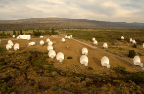
Figure 2: The Allen Telescope Array. Image courtesy of Seth Shostak and the SETI institute.

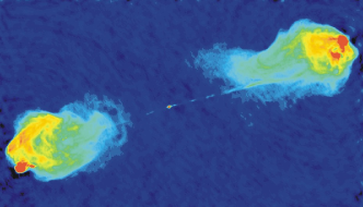
Figure 3: Cygnus A image. False color image of the radio jet and lobes in the hyperluminous radio galaxy Cygnus A. Red shows regions with the brightest radio emission, while blue shows regions of fainter emission. Image courtesy of NRAO/AUI by Perley et al. [8].

In 1962 the principle of synthesis aperture imaging using earth rotation was proposed by Ryle [9]. Ryle’s idea was simple and beautiful. Instead of moving the antennas as he has been doing for about 15 years, he used the fact that the earth rotates to generate the synthetic aperture. This quickly became the main operating mode of radio interferometers. However, imaging using earth rotation synthesis radio telescopes is an ill-posed problem due to the irregular sub-Nyquist sampling of the Fourier domain. This sub-sampling results in aliasing inside the image due to the high sidelobes of the array response. To solve this problem we need to remove the effect of the instrumental response from the image (a process known as deconvolution) and to compensate for inaccuracies in the array response (known as self calibration, but it has many similarities to blind deconvolution). It is important to understand that the improved imaging capability is a result of better equipment in conjunction with new imaging techniques. Each generation of radio telescopes involved significant hardware development effort. However, exploiting the hardware capabilities requires a constant improvement in imaging and self calibration to match the receiver sensitivity. Figure 3 (By Perley et al. [8])presents the outcome of imaging and self calibration applied to an image of Cygnus A. It is the first discovery of the radio jets going from the center all the way to the external radio lobes. Even though Cygnus A has been observed for many years (since Reber’s time) it is the image formation and self calibration algorithms that allowed the discovery of the radio jets.

Over the last 40 years many deconvolution techniques have been developed to solve this problem. The basic idea behind a deconvolution algorithm is to exploit a-priori knowledge about the image. The first algorithm and the most popular of these techniques is the CLEAN method proposed by Högbom [10]. The maximum entropy algorithm (MEM) with various entropy functions was proposed in [11], [12], [13] and [14] and the current implementation by Cornwell and Evans [15] is the most widely used. Beyond these two techniques there are several extensions in various directions: extensions of the CLEAN algorithm to support multi-resolution and wavelets as well as non co-planar arrays and multiple wavelengths (see the overview paper [16]). MEM techniques have been also extended to take into account source structure through the use of multiresolution and wavelet based techniques [17]. Global non-negative least squares was proposed by Briggs [18], matrix based parametric imaging such as the Least Squares Minimum Variance Imaging (LS–MVI) and maximum likelihood based techniques in [19] and [20] and sparse $L_{1}$ reconstruction in [21] and [22]. Source modeling is an important issue and various techniques to improve modeling over simple point source models by using shapelets, wavelets and Gaussians [23] have been implemented. A more extensive overview of classical techniques and implementation issues is given in [24] or [25].

Better performance analysis of imaging as well as self calibration techniques is one of the major challenges for the signal processing community. This is likely to become a more critical problem for the future generation of radio interferometers that will be built in the next two decades such as the square kilometer array (SKA), the Low Frequency Array (LOFAR), the Allen Telescope Array (ATA, see figure 2), the Long Wavelength Array (LWA) and the Atacama Large Millimeter Array (ALMA). These radio-telescopes will be composed of many stations (each station will be made up of multiple antennas that are combined using adaptive beamforming). These radio-telescopes will have significantly increased sensitivity and bandwidth, and some of them will operate at much lower frequencies than existing radio telescopes. Improved sensitivity will therefore require a much better calibration, the capability to perform imaging with much higher dynamic range in order to reduce the effect of the residuals of powerful foreground sources inside and outside the field of view and better handling of non-coplanar arrays.

The structure of the paper is as follows: We begin with a description of the basic imaging equation and a parametric reformulation of the problem. The basic approaches to imaging, assuming a calibrated array are described next. We then describe some modifications of the parametric imaging techniques that make it possible to combine imaging and calibration through semi-definite programming. We end up with some simulated and measured examples.

II The imaging equations

This section reviews the basic principles of radio astronomy following Taylor et al. [25]. In radio astronomy we observe the radio waves emitted from space. Since the source is far away, the received electromagnetic field intensity distribution can be observed only in an angular direction (no information regarding the intensity distribution in the radial direction). Defining the celestial sphere as the maximal sphere that contains no radiating sources, the observed intensity is the projection of the source intensity on the celestial sphere. For simplicity we will deal with a quasi monochromatic wave at frequency $\nu$ (the general case can be easily derived by a linear combination of quasi monochromatic waves). The electric field at location ${\bf r}$ is given by:

$$E_{\nu}({\mathbf{r}})=\int\epsilon_{\nu}({\bf q})\frac{e^{2\pi\jmath\nu\left|\bf{q}-{\mathbf{r}}\right|/c}}{\left|\bf{q}-{\mathbf{r}}\right|}{\rm d}S$$ (1)

where $\epsilon_{\nu}(\bf{q})$ is the electric field at location $\bf{q}$ (on the celestial sphere), ${\rm d}S$ is surface area on the sphere and the integration is done over the entire sphere and $c$ is the speed of light.

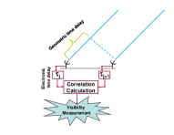
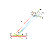
Figure 4: Measurement setting. 4 - The visibility is the measurement of spatial correlation between the electric field of antenna pairs. The geometric delay of the wave that propagates from the source to the two antennas is compensated for by an electronic delay. 4 - A distant source is observed by an antenna pair. The baseline connecting the two antennas is the origin of the $(u,v,w)$ coordinate system. The $w$ axis points from the baseline toward the source reference point. $(u,v)$ are perpendicular to $w$ and selected according to the Earth’s orientation. $(l,m,n)$ is a unit vector in the $(u,v,w)$ system pointing toward a specific location in the source (at the source reference point $S_{o}$, $l=0,m=0$ ) and $n=\sqrt{\left(l^{2}+m^{2}\right)}$.

For two antennas observing a distant source (receiving the electric field emitted by the source) there is a geometrical delay in one of the antennas relative to the other antenna derived from the source observation angle (see Figure 4); if the geometric delay is compensated by an electronic delay, the electric field received in one antenna should be highly correlated with the electric field received by the other antenna. The spatial coherency of the electric field for two antennas located at ${\bf r}_{1}$ and ${\bf r}_{2}$ is given by

$$V_{\nu}(\bf{r_{1}},\bf{r_{2}})=\langle\bf{E}_{\nu}({\bf r}_{1})\bf{E}^{*}_{\nu}({\bf r}_{2})\rangle.$$ (2)

where $\langle\rangle$ stands for the expectation value. Substituting (1) into (2) and taking into account the large distance of the source; i.e. $\left|\bf{q-r}\right|\approx\left|\bf{q}\right|$ and that the electric field is spatially incoherent (i.e., $\langle\epsilon_{\nu}({\bf q}_{1})\epsilon^{*}_{\nu}({\bf q}_{2})\rangle=0\phantom{a}\forall{{\bf q}_{1}}\neq{{\bf q}_{2}}$) we get

$$V_{\nu}({\bf r}_{1},{\bf r}_{2})=\int I_{\nu}(s)e^{-2\pi\jmath\nu{\bf s}({\bf r}_{1}-{\bf r}_{2})/c}d\Omega,$$ (3)

where $I_{\nu}({\bf s})\equiv\langle\epsilon_{\nu}({\mathbf{s}})^{2}\rangle$ is the source intensity at direction $\bf s$ on the sphere ($\bf s\equiv\frac{\bf q}{|\bf q|}$), and $d\Omega=\frac{dS}{|{\bf q}|^{2}}.$ Representing (3) in the $(u,v,w)$ coordinate system, for many astronomical observations (e.g., planar arrays, or small field of view imaging) we obtain

$$V_{\nu}(u,v)=\int\int I_{\nu}(l,m)e^{-2\pi\jmath(ul+vm)}{\rm d}l{\rm d}m.$$ (4)

The visibility is the Fourier transform of the source intensity; therefore the inverse relation holds :

$$I_{\nu}(l,m)=\int\int V_{\nu}(u,v)e^{2\pi\jmath(ul+vm)}{\rm d}u{\rm d}v.$$ (5)

When the co-planar approximation does not hold, equation (4) takes the more complicated form

$$V_{\nu}(u,v,w)=\int\int\frac{1}{n}I_{\nu}(l,m)e^{-2\pi\jmath\left[ul+vm+w(n-1)\right]}{\rm d}l{\rm d}m,$$ (6)

where

$$n\equiv\sqrt{1-\ell^{2}-m^{2}}.$$ (7)

For a source with visibility measurements covering the entire $(u,v)$ domain, the source image is perfectly computed by the Fourier inversion of the visibility. In practice, only a small part of the $(u,v)$ domain is measured by sampling the existing antenna pair baselines as they change with the Earth’s rotation relative to the $(u,v)$ coordinates (at time $t_{k}$ two antennas $p$ and $q$ measure a single visibility point in the $(u,v)$ domain at $(u_{pq}^{k},v_{pq}^{k})$) . This set of samples is known as the $(u,v)$ coverage of the radio telescope. This coverage is determined by many factors such as the configuration in which the individual receptors (telescopes or dipole) are placed on the ground, the minimal and maximal distance between antenna pairs, the time difference between consecutive measurements and the total measurement time and bandwidth. An example of the $(u,v)$ coverage for a simulated radio telescope (East west array with 14 antennas logarithmically spaced from $\lambda$ to $200\lambda$, observation time of 12 hours) is shown in Figure 5. The sampled points in the $(u,v)$ plane are a collection of ellipses. The sampling effect on the resulting image is shown in Figure 6 and 6. Figure 6 depicts an image of visibility data measured over a dense and uniform grid in the $(u,v)$ plane (all grid points in the $(u,v)$ plane were sampled). Figure 6 presents the same data with a more realistic $(u,v)$ sampling. The image with the partial (and more realistic) measurement set is blurred, distorted and noisy. Let $S(u,v)$ be the sampling function ($S(u,v)=1$ for each measured $(u,v)$ pair and $S(u,v)=0$ otherwise). We obtain that the inverse direct Fourier transform of the measured visibility, known as the dirty image $I_{D}$ is given by:

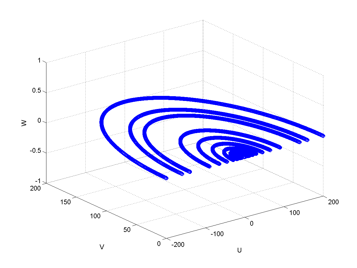
Figure 5: $(u,v)$ coverage of a simulated East-West radio telescope with 14 antennas logarithmically spaced with baselines up to 200$\lambda$. Observations are made every 6 minuets for a duration of 12 hours. From each antenna pair we get an ellipse in the $(u,v)$ domain. $u$ and $v$ are in $\lambda$ units.

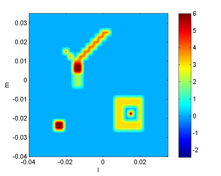
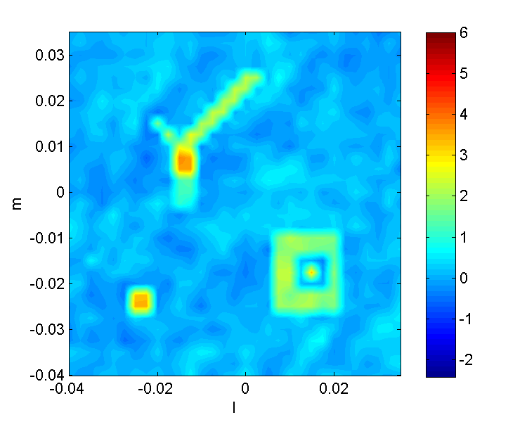
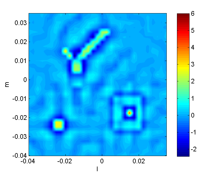
Figure 6: Illustration of sampling and gridding effects. 6: Fourier transform of visibility data on a perfect grid (visibility measurements location are on the center of the grid cells) with complete $(u,v)$ coverage. 6: Fourier transform of visibility data with off-grid points (the visibility measurements location were chosen randomly) and complete $(u,v)$ coverage, demonstrates gridding effect. Features in the image are blurred and distorted. 6: Fourier transform of visibility data with perfect grid and incomplete $(u,v)$ coverage (of the radio telescope described in Figure 5), demonstrates the sampling effect.

$$I_{D,\nu}(l,m)=\int\int V_{\nu}(u,v)S(u,v)e^{2\pi\jmath(ul+vm)}{\rm d}u{\rm d}v.$$ (8)

The instrument point spread function which is also known as the dirty beam is defined by:

$$B(l,m)\equiv\int\int S(u,v)e^{2\pi\jmath(ul+vm)}{\rm d}u{\rm d}v.$$ (9)

By the convolution theorem, the dirty image is the convolution of the true source intensity (5) and the dirty beam (9):

$$I_{D,\nu}=I_{\nu}*B$$ (10)

This is the reason why image reconstruction algorithms in radio astronomy are often referred to as deconvolution algorithms, since direct synthesis produces $I_{D,\nu}$, but we want to obtain $I_{\nu}$ by deconvolution with respect to $B$. The dirty image can be calculated from the measured visibility data according to equation (8), or by using a Fast Fourier Transform (FFT) to reduce the calculation time and memory resources. In order to use the FFT, the visibility data must lie on a rectangular equally spaced grid. This procedure of re-sampling the measured visibilities on a regular grid is called gridding. The weighting is done by convolving the visibilities with a smooth kernel (this procedure is also called convolutional gridding). Choice of the gridding kernel is important and follows from standard interpolation theory. An illustration of the gridding effect for a rectangular kernel is shown in Figures 6 and 6. Both images were generated using simulated visibility data with complete $(u,v)$ coverage. In Figure 6 the visibility data were taken on a perfect grid (all visibility measurements were located on the center of a grid cell). In Figure 6 the location of the visibility measurements was chosen randomly within the cells in the $(u,v)$ plane). This results in a blurred and distorted image. For more details on gridding and tapering the reader is referred to [24] and [25].

III The parametric matrix formulation of the image formation problem

We now describe an alternative formulation of the image formation problem. In this formulation imaging is viewed as a parameter estimation problem, where the locations and powers (and possibly polarization parameters and frequency dependence of power) are the unknown parameters. This formalism was first proposed in [26] and [19] to allow for the introduction of interference mitigation techniques in the imaging process. It was extended to non co-planar array and polarimetric imaging in [20]. This formulation also allows easy inclusion of space dependent calibration parameters [27]. Assume that the observed image is a collection of $D$ point sources, i.e.,

$$I_{\nu}(l,m)=\sum_{d=1}^{D}I_{\nu}(l,m)\delta(l-l_{d})\delta(m-m_{d}).$$ (11)

Since $(u,v)$ are the baseline coordinates (i.e. $u\equiv u_{ij}^{k}=u_{i}^{k}-u_{j}^{k}$ and $v\equiv v_{ij}^{k}=v_{i}^{k}-v_{j}^{k}$), the visibility (4) can be rewritten as

$$V_{\nu}(u_{ij}^{k},v_{ij}^{k})=\sum_{d=1}^{D}I_{\nu}(l_{d},m_{d})e^{-2\pi\jmath(u_{ij}^{k}l_{d}+v_{ij}^{k}m_{d})}.$$ (12)

where $k$ denotes the measurement time $t_{k}$. Selecting a (time varying) reference point at one of the antennas $(u_{0}^{k},v_{0}^{k})$ and manipulating (12) yields

$$\begin{array}[]{lcl}V_{\nu}(u_{ij}^{k},v_{ij}^{k})&=&\sum_{d=1}^{D}e^{-2\pi\jmath(u_{i,0}^{k}l_{d}+v_{i,0}^{k}m_{d})}I_{\nu}(l_{d},m_{d})\\ &&e^{2\pi\jmath(u_{j,0}^{k}l_{d}+v_{j,0}^{k}m_{d})}\end{array}$$ (13)

We define the $k$’th measurement correlation matrix ${\mathbf{R}}_{k}$ by:

$$({\mathbf{R}}_{k})_{ij}\equiv V_{\nu}(u_{ij}^{k},v_{ij}^{k})$$ (14)

The correlation matrix is illustrated in Figure 7, for a single frequency bin. Cell $R_{ij}^{k}$ of the correlation matrix is the visibility measurement at time $t_{k}$ from antenna pair $(i,j)$. The size of the correlation matrix ${\mathbf{R}}_{k}$ is $p\times p$ where $p$ is the number of antennas in the array. The autocorrelation of each antenna is also used (the diagonal of the correlation matrix). When an observation uses more than a single frequency bin, each correlation matrix is computed using a single bin as illustrated in Figure 8.

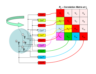
Figure 7: The correlation matrix (for the simple case of a single frequency) in a specific time measurement $t_{k}$ is built from the visibility measurement of antenna pairs

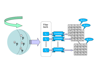
Figure 8: The correlation matrices for an observation in the multi frequency case. The correlation matrices are calculated for each frequency separately (on filtered measurements from the antennas).

Let the Fourier component vector at time $t_{k}$ be:

$${\bf a}_{k}(l,m)\equiv\left(\begin{array}[]{c}e^{-2\pi\jmath(u_{1,0}^{k}l+v_{1,0}^{k}m)}\\ \vdots\\ e^{-2\pi\jmath(u_{p,0}^{k}l+v_{p,0}^{k}m)}\\ \end{array}\right),$$ (15)

and let the Fourier component matrix at time $t_{k}$ be

$${\mathbf{A}}_{k}\equiv\left[\begin{array}[]{ccc}{\bf a}_{k}(l_{1},m_{1}),&\ldots&,{\bf a}_{k}(l_{d},m_{d})\\ \end{array}\right].$$ (16)

Define the point source intensity matrix by :

$${\mathbf{B}}\equiv\left[\begin{array}[]{ccc}I(l_{1},m_{1})&&0\\ &\ddots&\\ 0&&I(l_{D},m_{D})\\ \end{array}\right].$$ (17)

Using (15)-(17) equation (13) can be rewritten as

$${\mathbf{R}}_{k}={\mathbf{A}}_{k}{\mathbf{B}}{\mathbf{A}}_{k}^{H}.$$ (18)

Matrix equation (18) is the parametric form of the classical equation (4). It will allow us to consider the problem as an estimation problem, where we observe a set of measured covariance matrices which depend smoothly on the unknown source and instrument calibration parameters, as well as receiver noise. Using this formulation we can easily use well-known techniques from estimation theory (such as maximum a-posteriori, ML, MVDR and robust techniques) to solve the image formation problem. It also enables a simple extension to the non-coplanar array case as well as polarimetric imaging and multi-frequency synthesis, where sources have frequency dependent (parametrically known) characteristics. The classical dirty image (8) can be rewritten as

$$I_{D}(l,m)=\frac{1}{K}\sum_{k}{\mathbf{a}}_{k}^{H}(l,m){\mathbf{R}}_{k}{\mathbf{a}}_{k}(l,m).$$ (19)

Note that this is identical to the mean power output of a classical beamformer oriented towards direction $(l,m)$. More realistically, the antenna response varies slightly between different antennas and there is an additional noise per antenna. The antenna response can be measured prior to the observation and taken into account in the model. Since the noise in two antennas is independent, the noise correlation matrix is diagonal. Denoting by $\gamma_{i,k}$ the unknown complex gain of antenna $i$ at observation time $t_{k}$ and by $\sigma^{2}$ the noise variance, the correlation matrix now becomes:

$${\mathbf{R}}_{k}=\mbox{$\mbox{\boldmath$\Gamma$}$}_{k}{\mathbf{A}}_{k}{\mathbf{B}}{\mathbf{A}}_{k}^{H}\mbox{$\mbox{\boldmath$\Gamma$}$}_{k}^{H}+\sigma^{2}{\mathbf{I}}$$ (20)

where

$$\mbox{$\mbox{\boldmath$\Gamma$}$}_{k}\equiv\left[\begin{array}[]{ccc}\gamma_{1,k}&&0\\ &\ddots&\\ 0&&\gamma_{p,k}\\ \end{array}\right]$$

Estimation of the $\gamma_{i,k}$ is discussed in a companion paper by Wijnholds et al. [28]. Note that typically $\gamma_{i,k}$ varies slowly so it can be assumed to be constant over multiple times. Similarly, the non-coplanar array case is given by replacing ${\mathbf{a}}_{k}$ and ${\mathbf{B}}$ by

$$\begin{array}[]{ll}{\mathbf{a}}_{k}(l,m)&\equiv\\ \left[e^{-2\pi\jmath(u_{1,0}^{k}l+v_{1,0}^{k}m+w_{1,0}^{k}n)},...,e^{-2\pi\jmath(u_{p,0}^{k}l+v_{p,0}^{k}m+w_{1,0}^{k}n)}\right]^{T}\end{array}$$ (21)

and

$${\mathbf{B}}\equiv\left[\begin{array}[]{ccc}\frac{I(l_{1},m_{1})}{\sqrt{1-\ell_{1}^{2}-m_{1}^{2}}}&&0\\ &\ddots&\\ 0&&\frac{I(l_{D},m_{D})}{\sqrt{1-\ell_{D}^{2}-m_{D}^{2}}}\\ \end{array}\right].$$ (22)

The radio imaging problem can now be reformulated as follows: Given a set of measured covariance matrices ${\mathbf{\hat{R}}}_{1},...,{\mathbf{\hat{R}}}_{K}$ estimate the parameters ${\mathbf{s}}_{1},...,{\mathbf{s}}_{D}$, $I({\mathbf{s}}_{1}),...,I({\mathbf{s}}_{D})$ and the calibration matrices $\mbox{$\mbox{\boldmath$\Gamma$}$}_{k}:k=1,...,K$. Note that (20) can be easily generalized to deal with direction dependent calibration parameters, polarized sources as well as multi-frequency synthesis. All that we need to change is the source and the calibration parametric model by simple adaptation of (20). The parametric approaches described in this paper can be applied uniformly to all these problems. However, for simplicity we will focus on the calibrated array case.

IV Classical and parametric approaches based on sequential source removal

Many algorithms in radio astronomy are based on sequential source removal. The most commonly used is the CLEAN algorithm originally proposed by Högbom [10]. These iterative algorithms assume that the observed field is a collection of sources with simple structure. CLEAN assumes that the sources are point sources. During each iteration a single point source is estimated and removed from the data. The reconstructed image is the collection of all point sources with their estimated power convolved with an ideal reconstruction beam (usually an elliptical Gaussian fitted to the central lobe of the dirty beam) . The general structure common to all the sequential source removal algorithms is described in Table I. The algorithms differ from each other by the exact definition of the dirty image used, the way the point source is removed from the image (either in the image domain after gridding or in the visibility domain), the intensity estimation method of the point sources and the exact modeling of the sources (point source, Gaussian, wavelet coefficients, shapelets, etc.). Some versions like the Cotton-Schwab technique estimate multiple sources based on the same dirty image. This significantly accelerates the algorithm, since the number of Fourier transforms of the image is reduced.

We describe two sequential source removal algorithms. The first is the CLEAN algorithm and the second is a parametric estimation based algorithm known as LS-MVI.

Initialization:

$\bullet$ Calculate the dirty image $I_{D}$ according to measured visibilities.

$\bullet$ Calculate the reconstruction beam $B_{rec}$ for later use.

While stopping criteria not met:

$\bullet$ Find the brightest location in the dirty image $(l_{i},m_{i})$.

This is the location of a new point source.

$\bullet$ Estimate the new point source intensity $\lambda_{i}$.

$\bullet$ Add the new point source to the source list.

(with the estimated intensity).

$\bullet$ Remove the new source response from the data

(both the dirty image and the visibility measurements).

Finalize:

$\bullet$ Calculate the reconstructed image $I_{rec}$

by convolving the source list with the reconstruction beam.

TABLE I: Generic source removal algorithm flow

IV-A The CLEAN Algorithm

The CLEAN algorithm assumes that the observed field of view is composed of point sources. Since the image of a point source is given by the convolution of the point source and the dirty beam (10), CLEAN iteratively removes the brightest point source from the image until the residual image is noise-like. There are several variants of CLEAN ([10],[29],[30],[31]). The CLEAN algorithm is implemented either in the image or in the visibility domain. In each iteration the brightest point in the dirty image (equation (8) ) is found (position and strength) and added to a point source list. A fraction of it ($\gamma$, $0<\gamma<1$) is removed from the dirty image. The $\gamma$ parameter is called the loop gain and is usually taken to be 0.1-0.2. The iterations continue until the residual image is noise like. The subtraction can be done either in the image domain or in the visibility domain. The visibility domain CLEAN is more accurate since we are not limited to pixel resolution. The algorithm flow for ungridded visibility domain CLEAN is summarized in Table II.

Initialization:

$\bullet$ Calculate $I_{D}$ (eq. 8).

$\bullet$ $i=0$.

$\bullet$ $B_{\rm rec}={\rm Gaussian}$.

While $I_{D}$ is not noise-like:

$\bullet$ $(l_{i},m_{i})={\rm arg}\max I_{D}(l,m)$.

$\bullet$ $\lambda_{i}=I_{D}(l_{i},m_{i})$.

$\bullet$ For all $p,q,k$:

$\tiny{V(u_{p,q}^{k},v_{p,q}^{k})=V(u_{p,q}^{k},v_{p,q}^{k})-\gamma\lambda_{i}e^{-2\pi j\left[u_{p,q}^{k}l_{i}+v_{p,q}^{k}m_{i}\right]}}$.

$\bullet$ Update $I_{D}$ (eq. 8).

$\bullet$ $i=i+1$.

Finalize:

$\bullet$ $I_{\rm rec}=I_{D}+\sum_{i}\gamma\lambda_{i}B_{\rm rec}(l-l_{i},m-m_{i})$.

TABLE II: Visibility domain CLEAN algorithm flow

An illustration of the CLEAN algorithm on a simulated image is shown in Figure (9). The simulated radio telescope is the same as in Figure (5). The loop gain used is $0.2$. In every iteration the strongest point source is found, added to the reconstructed image and subtracted from the dirty image. The loop gain serves three purposes. First, it prevents (or at least reduces) the effects of over-estimation of the power due to sidelobes from other sources. Second, it allows for interpolation of sources that are located off the grid. Third, it improves performance with extended sources. However, this limits the dynamic range of the image. The effect of pixelization and choice of grid on the dynamic range of the imaging process is further discussed in [32], [33]. Improved versions of CLEAN allow for estimation of location off the grid by using interpolation, and subtraction of the effect from the visibility rather than the dirty image. This has the positive effect of eliminating gridding accuracy effects. Acceleration of the CLEAN algorithm can be achieved by estimating multiple point sources based on a single dirty image (major cycle), as well as defining windows for the search procedure. Practically, defining windows reduces the size of the search space.

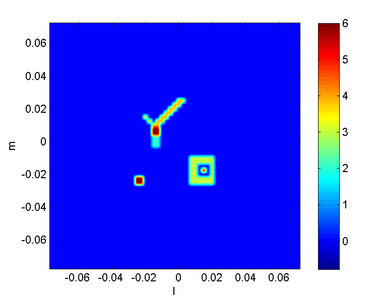
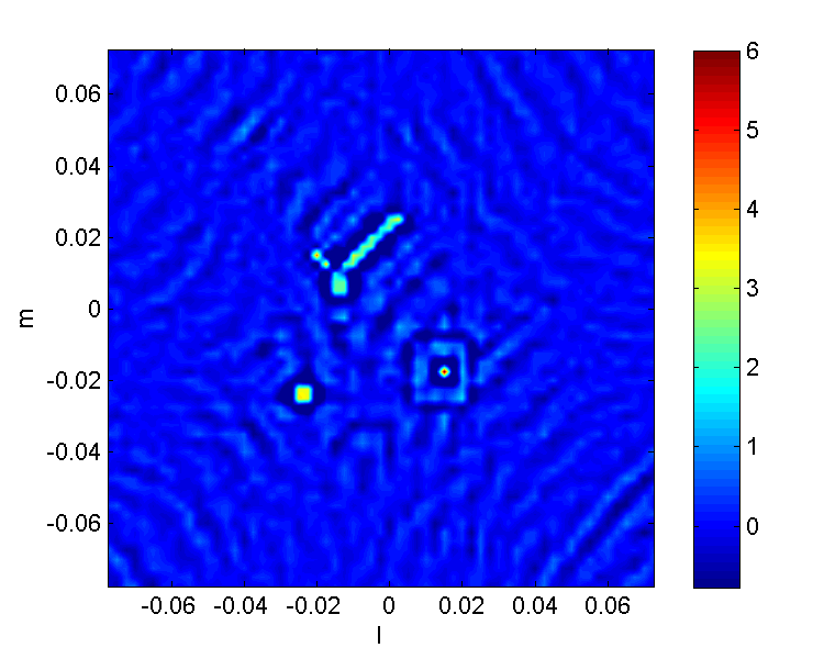
(a) Original Image	(b) Initial Dirty Image
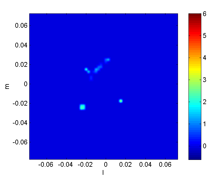
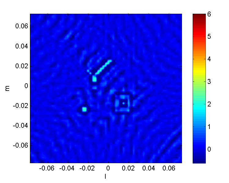
(c) Reconstructed Image - 50 iter	(d) Residual Image - 50 iter
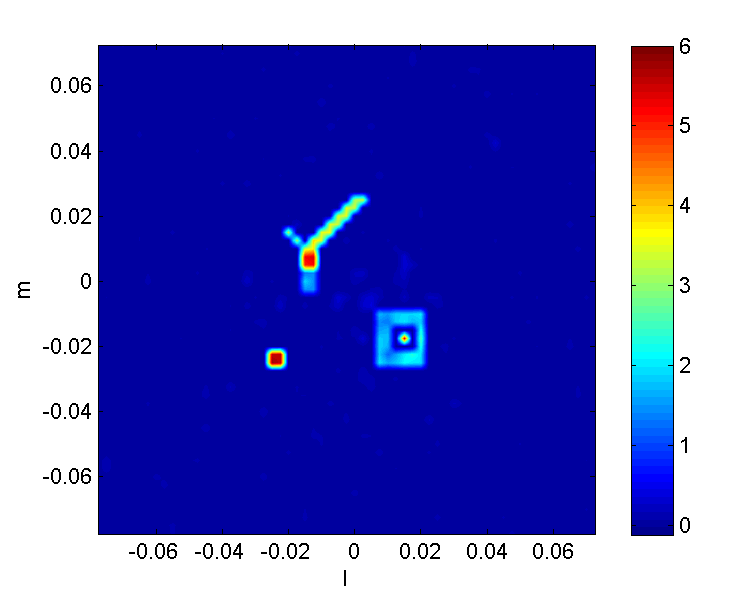
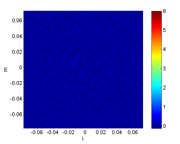
(e) Reconstructed Image - 25000 iter	(f) Residual Image - 25000 iter

Figure 9: CLEAN steps for a simulated image. (a) the original image. (b) the initial dirty image. (c) and (e) the reconstructed image after 50 and 25000 CLEAN iterations respectively. (d),(f) the residual dirty images after 50 and 25000 iterations respectively. In general, the sources are nicely reconstructed except from the square ring extended source. All images share the same color map. All images were up-sampled by 4 using Matlab basic interpolation.

IV-A1 Clark CLEAN Algorithm

One of the important variants of CLEAN was proposed by Clark in 1980 [30]. Clark’s algorithm main advantage is reduction of computational load. The algorithm is performed in two cycles, a major cycle and a minor cycle. A major cycle is constructed by selecting intensity limit value (according to a histogram of the dirty image values) and approximating a dirty beam (central patch of the true dirty beam) to be used during the subsequent minor cycles. A minor cycle consists of finding the brightest pixel in the image (i.e. a new point source) and removing a fraction of the point source response from the dirty image. In principle, the minor cycle is the same as described in the ’While’ loop in Table II, when the dirty beam used is only the centeral patch of the full dirty beam (hence computational complexity is significantly reduced). The inaccuracies caused by working with an approximated dirty beam are corrected during the major cycle. The Clark algorithm is performed in the visibility domain instead of the image domain, yielding a multiplication instead of a convolution for calculating the point source response.

IV-A2 Cotton Schwab Algorithm

Cotton & Schwab [31] developed a variant of the Clark CLEAN. Like the Clark CLEAN, in the Cotton Schwab CLEAN the procedure involves major and minor cycles. The main improvements over the Clark algorithm are that the Cotton Schwab algorithm calculation is done over the ungridded visibility data, thus avoiding gridding errors, and multi source removal is done independently in each minor cycle (from different fields). The CLEAN components from all fields are removed in the major cycle. Working with the ungridded visibility measurement is done using a measurement list as described in Table II. An element $V(u_{p,q}^{k},v_{p,q}^{k})$ of the measurement list is the measured visibility by an antenna pair $(p,q)$, corresponding to a baseline $(u_{p,q},v_{p,q})$ measured at time $k$.

IV-B The W-Projection algorithm

One of the main limitation of the previous technique is the case of non-coplanar arrays and large field of view. To overcome problems related to non-coplanar arrays the W-projection algorithm has been proposed by Cornwell et al. [34].

The W-projection algorithm deals with non-coplanar arrays i.e. when the planar approximation is violated and the imaging equation is given by equation (6). Originally Frater and Docherty [35] showed that a projection of visibility measurements from a constant $w$ plane to $w=0$ plane can be done. This corresponds to a radio telescope with antennas arranged in a plane with a single antenna outside the plane. In this case the measured visibilities are projected onto $w=0$ plane (real and imaginary part separately), a deconvolution is performed (such as CLEAN) and the resulting cleaned images are combined taking the constant $w$ value into account.

In the general case (projection of any $w$ values) the relation between $V(u,v,w)$ and $V(u,v,w=0)$ is given by

$$V(u,v,w)=\tilde{G}(u,v,w)*V(u,v,w=0)$$ (23)

where

$$G(l,m,w) \equiv e^{-2\pi j\left[w\left(\sqrt{1-l^{2}-m^{2}}-1\right)\right]}$$

$$\approx e^{\pi j\left[w\left(l^{2}+m^{2}\right)\right]}$$

$$\tilde{G}(u,v,w) = \frac{j}{w}e^{-\pi j\left[\frac{u^{2}+v^{2}}{w}\right]},$$

and $G(l,m,w)$ is the Fourier transform of $\tilde{G}(v,u,w)$ called the W-projection function. Given a model of the sky brightness, the visibility on the $w=0$ plane can be calculated using the two dimensional Fourier transform. The visibility measurement outside the $w=0$ plane may then be calculated using the convolution function $\tilde{G}(u,v,w)$. Note that representing the visibility as a convolution and using the FFT algorithm to compute the convolution is similar to the one-dimensional chirp z-transform algorithm. Calculating the image for a given set of visibility measurements is done using iterative algorithms since there is no inverse transform. The W-projection is a minor-major cycle algorithm that receives three dimensional visibility measurements $V(u,v,w)$ and projects the $w$ coordinate ’out’ (projection on $w=0$ plane). The 2D visibilities $V(u,v,w=0)$ are used to calculate the reconstructed image in the $(l,m)$ domain by a two dimensional Fourier Transform. Then a deconvolution is performed (such as CLEAN) on the resulting image. The W-projection algorithm has both high performance and high computational speed.

IV-C The LS-MVI algorithm

We now describe a recent approach that enables the use of modern array processing algorithms in the framework of image deconvolution. The method will be demonstrated on simulated and measured data. However, in contrast to the CLEAN algorithm it is in initial research stages and further development of the technique is an interesting research problem. The LS-MVI algorithm is a novel matrix based sequential source removal algorithm originally proposed in [19] and further improved in [20]. It is based on matrix based approach to direction-of-arrival (DOA) estimation techniques. We would like to replace the vectors ${\mathbf{a}}_{k}({\mathbf{s}})$ in (19) by a set of beamforming vectors ${\mathbf{w}}_{k}(s),k=1,...,K$. The main goal of the LS-MVI is to eliminate interference from other points in the image when estimating the location and power of a given source. To that end, filterbank techniques such as the MVDR and its extensions have proven very effective. Minimizing the interference from sidelobes of the dirty beam while observing a point source in direction ${\mathbf{s}}=(l,m)$ can be formulated as a constrained beamforming problem (For simplicity we denote ${\mathbf{w}}_{k}({\mathbf{s}})$ by ${\mathbf{w}}_{k}$ and assume that ${\mathbf{w}}=\left[{\mathbf{w}}_{1},...,{\mathbf{w}}_{K}\right]^{T}$).

$$\begin{array}[]{l}{\mathbf{\hat{w}}}({\mathbf{s}})\;=\;\mathop{\operator@font arg\,min}_{{\mathbf{w}}}\;\sum_{k=1}^{K}{\mathbf{w}}_{k}^{\raisebox{1.0pt}{$\rm\scriptscriptstyle H$}}{\mathbf{\hat{R}}}_{k}{\mathbf{w}}_{k}\\ \qquad\hbox{\ subject to \ }\\ \sum_{k=1}^{K}{\mathbf{w}}_{k}^{\raisebox{1.0pt}{$\rm\scriptscriptstyle H$}}{\mathbf{a}}_{k}({\mathbf{s}})=1\,.\end{array}$$ (25)

The solution is given by

$$\begin{array}[]{l}{\mathbf{\hat{w}}}_{k}({\mathbf{s}})=\beta({\mathbf{s}}){\mathbf{\hat{R}}}_{k}^{-1}{\mathbf{a}}_{k}({\mathbf{s}}),\\ \end{array}$$ (26)

where, $\beta({\mathbf{s}})=\frac{1}{\sum_{k=1}^{K}{\mathbf{a}}_{k}^{\raisebox{1.0pt}{$\rm\scriptscriptstyle H$}}({\mathbf{s}}){\mathbf{\hat{R}}}_{k}^{-1}{\mathbf{a}}_{k}({\mathbf{s}})}$, ${\bf a}_{k}({\mathbf{s}})$ is given in equation (15) and ${\mathbf{\hat{R}}}_{k}$ is the covariance matrix measured at time $t_{k}$. The vectors ${\mathbf{\hat{w}}}({\mathbf{s}})$ have different magnitudes for different values of ${\mathbf{s}}$. This is undesirable since it generates noise related spatial features. Therefore, the adapted angular response (AAR) solution normalizes the norm of ${\mathbf{w}}$ to 1. The resulting solution is given by

$$\begin{array}[]{lcl}I_{D}^{\rm AAR}(l,m)&\equiv&\frac{\sum_{k=1}^{K}{\bf a}_{k}(l,m)^{H}{\mathbf{\hat{R}}}_{k}^{-1}{\bf a}_{k}(l,m)}{\sum_{k}{\bf a}_{k}(l,m)^{H}{\mathbf{\hat{R}}}_{k}^{-2}{\bf a}_{k}(l,m)}.\end{array}$$ (27)

This modified dirty image replaces the classical dirty image in the LS-MVI deconvolution process.

The intensity estimation used by the LS-MVI algorithm is a LS estimation of a point source at location $(l,m)$ and given by the following equation:

$$\begin{array}[]{ll}\alpha&={\rm arg}\min_{\alpha}\sum_{k}\|{\mathbf{\hat{R}}}_{k}-\alpha{\bf a}_{k}(l,m){\bf a}_{k}^{H}(l,m)\|_{F}^{2}\\ &\text{subject to }\alpha\geq 0\end{array}$$ (28)

This estimate of the source power has been independently used in ASP-CLEAN [36]. The closed form solution of equation (28) is given by

$$\alpha=\max\left\{\frac{{\bf h}^{H}{\mathbf{r}}}{{\bf h}^{H}{\bf h}},0\right\}.$$ (29)

where

$$h\equiv\left[vec({\mathbf{a}}_{1}(l,m){\mathbf{a}}_{1}^{H}(l,m))^{T},...,vec({\mathbf{a}}_{K}(l,m){\mathbf{a}}_{K}^{H}(l,m))^{T}\right]^{T}$$

and ${\mathbf{r}}\equiv\left[vec({\mathbf{\hat{R}}}_{1})^{T},...,vec({\mathbf{\hat{R}}}_{K})^{T}\right]^{T}$ are obtained by stacking the array response and the measured covariance matrices respectively.

The intensity estimation can be improved by adding the semi-definite constraint

$${\mathbf{\hat{R}}}_{k}-\sigma^{2}{\rm I}-\alpha{\bf a}_{k}(l,m){\bf a}_{k}^{H}(l,m)\succcurlyeq 0.$$ (30)

The intensity estimation is bounded between the solution (29) and $0$. Hence, a better intensity estimation can be achieved using a simple bi-section. A summary of the LS-MVI algorithm is given in Table (III). Another improvement that has low computational complexity is to use a joint LS estimate of all previously estimated sources. Assuming that we have collected $L$ components the estimator is given by:

$$\begin{array}[]{ll}\mbox{$\mbox{\boldmath$\alpha$}$}&={\arg}\min_{\mbox{$\mbox{\boldmath$\alpha$}$}}\sum_{k=1}^{K}||\small{{\mathbf{r}}_{k}-\sum_{i=1}^{L}\alpha_{i}{\mathbf{q}}_{ki}}||^{2}\\ &\text{s.t.}\alpha_{i}\geq 0{\hbox{\ for all \ }i}\end{array}$$ (31)

where $\mbox{$\mbox{\boldmath$\alpha$}$}=[\alpha_{1},...,\alpha_{L}]$, ${\mathbf{r}}_{k}=vec({\mathbf{R}}_{k})$ and ${\mathbf{q}}_{ki}=vec\left({\mathbf{a}}_{k}(l_{i},m_{i}){\mathbf{a}}_{k}^{H}(l_{i},m_{i})\right)$. Similarly to the CLEAN algorithm this improvement can be implemented only at major cycles, after several sources have been estimated.

Initialization:

$\bullet$ ${\mathbf{R}}_{k}^{0}={\mathbf{R}}_{k}$, $\forall k=1,\ldots,K$

$\bullet$ Calculate $I_{D}^{\rm AAR}$ using eq. (27)

$\bullet$ $i=0$

$\bullet$ $B_{\rm rec}={\rm Gaussian}$

While $I_{D}$ is not noise like:

$\bullet$ $(l_{i},m_{i})={\rm arg}\max I_{D}^{\rm AAR}(l,m)$

$\bullet$ Estimate $\alpha_{i}$ according to eq.(29)

$\bullet$ Optionally improve $\alpha_{i}$ estimation according to eq. (30)

$\bullet$ ${\mathbf{R}}_{k}^{i+1}={\mathbf{R}}_{k}^{i}-\gamma\alpha_{i}{\bf a}_{k}(l_{i},m_{i}){\bf a}_{k}^{H}(l_{i},m_{i})$, $\forall k=1\ldots K$

$\bullet$ Calculate $I_{D}^{\rm AAR}$ using ${\mathbf{R}}_{k}^{i+1}$ using eq. (27)

$\bullet$ $i=i+1$

Finalize:

$\bullet$ $I_{\rm rec}=\sum_{i}\gamma\alpha_{i}B_{\rm rec}(l-l_{i},m-m_{i})$

TABLE III: LS-MVI algorithm flow

There are two main differences between LS-MVI and CLEAN. First, the LS-MVI uses a different type of dirty image and second, the LS-MVI performs a more sophisticated intensity estimation than CLEAN. The dirty image used by the LS-MVI is $I_{D}^{\rm AAR}$ given in equation (27). The main advantage of the AAR dirty image over simple MVDR is the isotropic noise response that prevents the formation of spatially varying noise related artifacts. In [20] further extensions for enforcing semi-definite constraints in a Cotton-Schwab type of iteration are also presented. It should also be noted that there is no need to compute the complete dirty image in order to find the maximum and optimization techniques can do this much faster, especially if the user can provide windows similar to CLEAN windows currently used by radio astronomers. Like CLEAN, the LS-MVI should be implemented in the visibility domain to eliminate gridding effects.

V Global optimization based techniques

We now turn to a second family of solutions to the image formation problem. These solutions are based on optimizing a global property of the image subject to goodness of fit to the data. They vary from least squares (LS) based techniques to maximum entropy and $\ell_{1}$ based reconstruction.

V-A Linear deconvolution

Computationally the simplest way to solve the image formation problem is through linear inversion. There are two main approaches in this area: The well known Least Squares (LS) technique and Linear Minimum Mean Square Error (LMMSE). Such techniques can work well when the $(u,v)$ coverage is good and the inversion is well conditioned. Furthermore linear inversion can work independently of the complexity of the source structure. However, linear techniques can result in significant noise enhancement in ill-posed problems. For a fully sampled visibility domain, these techniques can provide a first approximation to the image. To overcome this problem one can use a constrained LS, also known as non-negative LS (NNLS), first proposed for radio synthesis imaging by Briggs [18]. The idea is that the image is positive. Putting these constraints into the deconvolution, yields a computationally expensive, though feasible algorithm. An excellent overview of the implementation of the NNLS can be found in [18].

V-B Maximum Entropy image reconstruction

The maximum entropy image formation technique is one of the two most popular deconvolution techniques in radio astronomy (together with CLEAN). The maximum entropy principle was first proposed by Jaynes [37]. A good overview of the philosophy behind the idea can be found in [38]. Since then it has been used in a wide spectrum of imaging problems. The basic idea behind MEM is the following: Out of all the images which are consistent with the measured data where the noise distribution does not satisfy the positivity demand,i.e., the sky brightness is a positive function, consider only those that satisfy the positivity demand. From these select the one that is most likely to have been created randomly. This idea was also proposed by [11] for optical images and applied to radio astronomical imaging in [12]. Other approaches based on differential entropy have also been suggested [13] and [14]. An extensive collection of papers discussing these different methods and aspects of maximum entropy can be found in a number of papers in [39]. [40] provides an overview of various maximum entropy techniques and the use of the various options for choosing the entropy measure. Interestingly, in that paper, a closed form solution is given for the noiseless case, but not for the general case.

The approach in [12] begins with a prior image and iterates between maximizing the entropy function and updating the $\chi^{2}$ fit to the data. The computation of the image based on a prior image is done analytically, but at each step the model visibilities are updated, through a two-dimensional Fourier transform. This type of algorithm is known as a fixed point algorithm, since it is based on iterating a function until it converges to a fixed point.

The maximum entropy solution is given by solving the following Lagrangian optimization problem [12]:

$$I^{MEM}=\arg\max_{I}-\sum_{l,m}I(l,m)\log\frac{I(l,m)}{F(l,m)}-\frac{\lambda}{2}\chi^{2}(V),$$ (32)

where

$$\chi^{2}(V)=\sum_{(u,v)\in A}\frac{1}{\sigma^{2}}\left|{{\hat{V}}}(u,v)-V(u,v)\right|^{2},$$ (33)

$V(u,v)$ are the model based visibilities, $\lambda$ is a Lagrange multiplier for the constraint that $V(u,v)$ should match the measured visibilities ${{\hat{V}}}(u,v)$, $A$ is the $(u,v)$ coverage of the radio telescope and $F(l,m)$ is a reference image. Taking the derivative with respect to $I(l,m)$ we obtain that the solution is given by:

$$I(l,m)=exp\left(-1+\log F(l,m)+\lambda\Delta(l,m)\right)$$ (34)

where

$$\Delta(l,m)=\sum_{(u,v)\in A}\frac{1}{\sigma^{2}}Re\left(\left({{\hat{V}}}(u,v)-V(u,v)\right)e^{\frac{\jmath 2\pi(ul+vm)}{N}}\right).$$

The basic maximum entropy algorithm now proceeds by choosing an initial image model (typically a flat image or a low resolution image) computing the model based visibilities $V(u,v)$ on a grid $A$. Using these visibilities a new model image is computed by equation (34). New visibilities are computed from the new model and the process is iterated until convergence.

While it is known that for the maximum entropy, this approach usually converges, the convergence can be slow [40]. Improved methods based on the Newton method and the Conjugate Gradient technique were put forward by [15, 41, 42]. These methods perform direct optimization of the entropy function subject to the $\chi^{2}$ constraint. Generalization of the maximum entropy using wavelets and multi-resolution techniques have also been proposed (see e.g., [17], [43]).

V-C Compressed sensing and sparse reconstruction techniques

Recently there has been growing interest in using $\ell_{1}$ based cost functions for deconvolution (see [21] and [22] and unpublished notes by Schwardt). This renewed interest in $\ell_{1}$ comes from recent results related to compressed sampling using Fourier bases. It is worth noting that as early as 1987 Marsh and Richardson [44] proved that the CLEAN algorithm can be regarded as an $\ell_{1}$ minimization for a single point source image. $\ell_{1}$ is not the only criterion. Recovery of noisy and blurred images using total variation ($TV$) optimization for smooth images was discussed by Dobson and Santosa [45]. Chen et al. [46] dealt with $\ell_{1}$ minimization of an image basis to achieve image sparseness using linear programming. Feuer and Nemirovski [47] and Elad and Bruckstein [48] established sufficient and necessary conditions for replacing $\ell_{0}$ optimization (computing the sparsest solution with high computational complexity) by linear programming when searching for the unique sparse representation. Rudelson and Vershynim [49] proved the best known guarantees for exact reconstruction of a sparse signal from its Fourier measurements.

Radio astronomical image reconstruction is done based on the visibility measurement in the $(u,v)$ domain. Reconstruction of the source image $I(l,m)$ is equivalent to estimating the missing visibility points. The missing $V(u,v)$ measurements together with the image itself are estimated by minimizing a cost function $||I(l,m)||_{\ell_{1}}$ in the $(l,m)$ domain using the constraints of image positivity and the measured visibility data. Note that since $I(l,m)$ is a positive quantity we have:

$$||I(l,m)||_{\ell_{1}}=\sum_{l=1}^{N}\sum_{m=1}^{N}I(l,m)$$ (35)

which allows us to use linear programming. To solve the reconstruction problem fast, we represent the problem as a linear programming problem with real variables. To that end let $\langle\cdot,\cdot\rangle$ be a one-to-one pairing function mapping $\left\{0,...,N-1\right\}\times\left\{0,...,N-1\right\}$ onto $\left\{0,...,N^{2}-1\right\}$. Let ${\mathbf{F}}$ be an $N^{2}\times N^{2}$ matrix whose elements satisfy

$${\mathbf{F}}_{\langle l,m\rangle,\langle u,v\rangle}=e^{\frac{-2\pi\jmath}{N}\left(ul+vm\right)}.$$ (36)

Let $\mbox{$\mbox{\boldmath$\xi$}$}=\hbox{vec}({\mathbf{V}})$ and let ${\mathbf{t}}=\hbox{vec}({\mathbf{I}})$. We have

$$\mbox{$\mbox{\boldmath$\xi$}$}={\mathbf{F}}{\mathbf{t}}.$$ (37)

Note that ${\mathbf{t}}$ is a real vector since the visibility measurements satisfy $V(u,v)={\bar{V}(-u,-v)}$. To make the problem real we define ${\mathbf{F}}_{R}=\hbox{Re}({\mathbf{F}}),{\mathbf{F}}_{I}=\hbox{Im}({\mathbf{F}})$ and variables $\mbox{$\mbox{\boldmath$\xi$}$}_{R}=\hbox{Re}(\mbox{$\mbox{\boldmath$\xi$}$}),\mbox{$\mbox{\boldmath$\xi$}$}_{I}=\hbox{Im}(\mbox{$\mbox{\boldmath$\xi$}$})$. (37) now becomes

$$\mbox{$\mbox{\boldmath$\xi$}$}_{R} = {\mathbf{F}}_{R}{\mathbf{t}}$$ (38)

$$\mbox{$\mbox{\boldmath$\xi$}$}_{I} = {\mathbf{F}}_{I}{\mathbf{t}}$$

For the measured locations $(u_{i},v_{i})$ we have:

$$\begin{array}[]{c}\mbox{$\mbox{\boldmath$\xi$}$}_{R}(\langle u_{i},v_{i}\rangle)=\hbox{Re}\left({{\hat{V}}}(u_{i},v_{i})\right)\quad i=1,...,M\\ \mbox{$\mbox{\boldmath$\xi$}$}_{I}(\langle u_{i},v_{i}\rangle)=\hbox{Im}\left({{\hat{V}}}(u_{i},v_{i})\right)\quad i=1,...,M\\ \end{array}$$ (39)

where $M$ is the number of given measurements in the $(u,v)$ domain. The linear programming problem is described in Table IV (for more details the reader is referred to [21]).

$\min_{{{\mathbf{t}}}}\sum_{i=1}^{N^{2}}{t_{i}}$
Subject to
$\mbox{$\mbox{\boldmath$\xi$}$}_{R}(\langle u_{i},v_{i}\rangle)=\hbox{Re}\left({{\hat{V}}}(u_{i},v_{i})\right)$
$\mbox{$\mbox{\boldmath$\xi$}$}_{I}(\langle u_{i},v_{i}\rangle)=\hbox{Im}\left({{\hat{V}}}(u_{i},v_{i})\right)$
$\mathbf{0}\leq{\mathbf{t}}$

TABLE IV: $\ell_{1}$ optimization using linear programming

In [22] a joint $\ell_{1}$ and $\ell_{2}$ is also discussed. This makes it possible to include prior knowledge on the noise power. Using the total variation is also a possibility that leads to $\ell_{1}$ optimization. Note that using total variation and maximum entropy are related since both functionals impose smoothness on the image.

VI Self calibration and robust MVDR for synthetic aperture arrays

We now turn to the case where the array response is not completely known, but we have some statistical knowledge of the error, e.g., we know the covariance matrix of the array response error at each epoch (measurement time). Typically this covariance will be time invariant or will have slow temporal variation. In this case we extend the robust dirty image as described in [50] to the synthetic aperture array case. This generalization follows the analysis in [20]. Since the positive definite constraint on the residual covariance matrices is important in our application we extended the robust Capon estimator of [51]. To that end assume that at each epoch we have an uncertainty ellipsoid describing the uncertainty of the array response (as well as unknown atmospheric attenuation). This is described by

$$\left({\mathbf{a}}_{k}({\mathbf{s}})-{\mathbf{\bar{a}}}_{k}({\mathbf{s}})\right)^{H}{\mathbf{C}}_{k}\left({\mathbf{a}}_{k}({\mathbf{s}})-{\mathbf{\bar{a}}}_{k}({\mathbf{s}})\right)\leq 1$$ (40)

where ${\mathbf{\bar{a}}}_{k}({\mathbf{s}})$ is the nominal value of the array response towards the point ${\mathbf{s}}$ and ${\mathbf{C}}_{k}$ are the covariance matrices of the uncertainty in the calibration parameters at time $k$. Generalizing the LS-MVI we would like to solve the following problem:

$$\begin{array}[]{ll}\left[\mbox{$\hat{\rho}$},{\mathbf{\hat{a}}}_{1},...,{\mathbf{\hat{a}}}_{k}\right]=\arg\max_{\rho,{\mathbf{a}}_{1},...,{\mathbf{a}}_{k}}\rho&\\ \hbox{subject to}&\\ {\mathbf{\hat{R}}}_{k}-\sigma^{2}{\mathbf{I}}-\rho{\mathbf{a}}_{k}{\mathbf{a}}_{k}^{H}\succeq\mathbf{0}&k=1,...,K\\ \left({\mathbf{a}}_{k}({\mathbf{s}})-{\mathbf{\bar{a}}}_{k}({\mathbf{s}})\right)^{H}{\mathbf{C}}_{k}\left({\mathbf{a}}_{k}({\mathbf{s}})-{\mathbf{\bar{a}}}_{k}({\mathbf{s}})\right)\leq 1&k=1,...,K\end{array}$$ (41)

Let $\tau=1/\rho$. The problem (41) is equivalent to the following problem

$$\begin{array}[]{ll}\left[\hat{\tau},{\mathbf{\hat{a}}}_{1},...,{\mathbf{\hat{a}}}_{k}\right]=\arg\min_{\tau,{\mathbf{a}}_{1},...,{\mathbf{a}}_{k}}\tau&\\ \hbox{subject to}&\\ \left[\begin{array}[]{cc}{\mathbf{\hat{R}}}_{k}-\sigma^{2}{\mathbf{I}}&{\mathbf{a}}_{k}\\ {\mathbf{a}}_{k}^{H}&\tau\end{array}\right]\succeq\mathbf{0}&k=1,...,K\\ \left[\begin{array}[]{cc}{\mathbf{C}}_{k}&\left({\mathbf{a}}_{k}({\mathbf{s}})-{\mathbf{\bar{a}}}_{k}({\mathbf{s}})\right)\\ \left({\mathbf{a}}_{k}({\mathbf{s}})-{\mathbf{\bar{a}}}_{k}({\mathbf{s}})\right)^{H}&1\end{array}\right]\succeq\mathbf{0}&k=1,...,K.\end{array}$$ (42)

This problem is once again a semi-definite programming problem that can be solved efficiently via interior point techniques [52]. We can now replace the MVDR estimator by this robust version. Interestingly, we obtain estimates of the corrected array response ${\mathbf{\hat{a}}}({\mathbf{s}}_{k})$. Using the model we obtain for each $k$

$${\mathbf{a}}_{k}({\mathbf{s}})=\mbox{$\mbox{\boldmath$\Gamma$}$}_{k}{\mathbf{\bar{a}}}_{k}({\mathbf{s}})$$ (43)

Hence, the self-calibration coefficients can be estimated using least squares fitting

$$\hat{}\mbox{$\mbox{\boldmath$\Gamma$}$}_{k}=\arg\min_{\gamma_{1},...,\gamma_{p}}\sum_{\ell=1}^{L}\|{\mathbf{\hat{a}}}_{k}({\mathbf{s}}_{\ell})-\mbox{$\mbox{\boldmath$\Gamma$}$}_{k}{\mathbf{\bar{a}}}_{k}({\mathbf{s}}_{\ell})\|^{2}$$ (44)

where $\mbox{$\mbox{\boldmath$\Gamma$}$}_{k}=\mathrm{diag}\{\gamma_{k,1},...,\gamma_{k,p}\}$. Of course, when the self-calibration parameters vary slowly we can combine the estimation over multiple epochs. This might prove instrumental in calibration of LOFAR type arrays, where the calibration coefficients vary across the sky. Since the computational complexity of the self-calibration semi-definite programming is higher than that of the MVDR dirty image, it is too complicated to solve this problem for each source in the image. Hence it should be used in a way similar to the external self-calibration cycle ([53]), where this problem is solved using a nominal source locations model. The advantage over ordinary self-calibration is that beyond the re-evaluation of the calibration parameters, we obtain better estimates of the source powers, without significant increase in the complexity. Another interesting alternative is to use the doubly constrained robust Capon beamformer which combines a norm constraint as in the AAR dirty image with robust Capon beamforming [54].

VII Examples and Comparisons

In this section we describe three examples of the various algorithms, including a simulated example of an extended source, an example from the LOFAR test station and an example of Abell 2256 observed by the VLA.

VII-A Simulated Extended Source

An extended source (Figure (10)) was simulated using an East-West array containing 10 antennas logarithmically spaced up to 1000$\lambda$. CLEAN deconvloution results are depicted in Figure (11 a) and (11 b). After 100 CLEAN iterations, the center of the source is partially reconstructed with distortion. After additional 20 iterations an artifact is generated (below the strong point on the right). This divergence can often occur in CLEAN when applying it to extended sources. The LS-MVI results are presented in Figure (11 c) and (11 d). After 100 iterations the center of the source is reconstructed and after 200 additional iterations and reconstruction is stable. The reason for this is the fact that CLEAN overestimate the power due to the high sidelobes level. Further analysis of this example is given in [20].

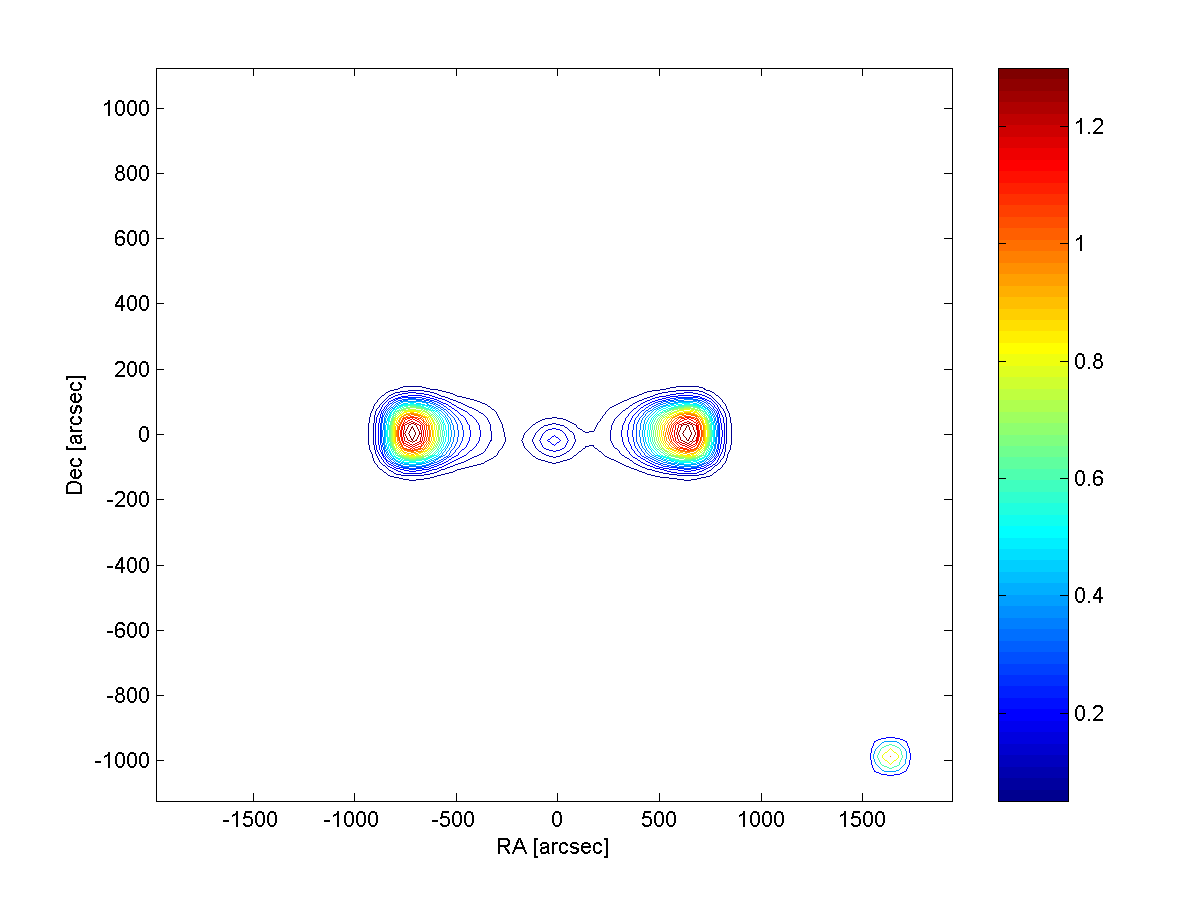
Figure 10: Original extended source image

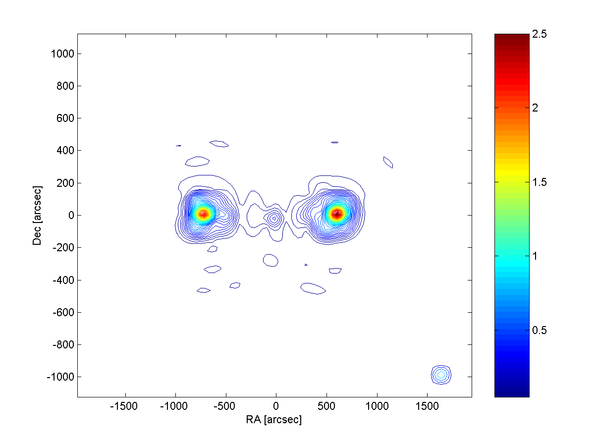
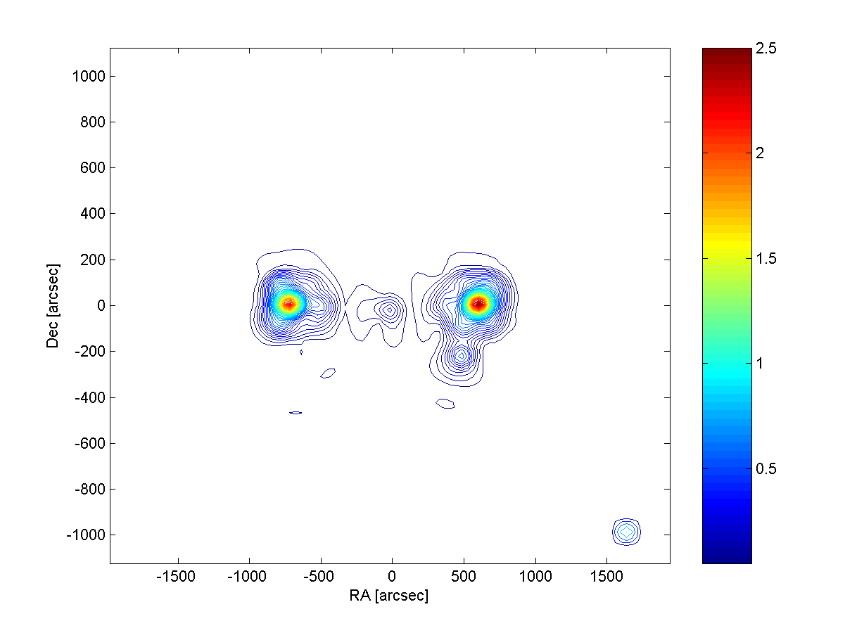
(a)	(b)
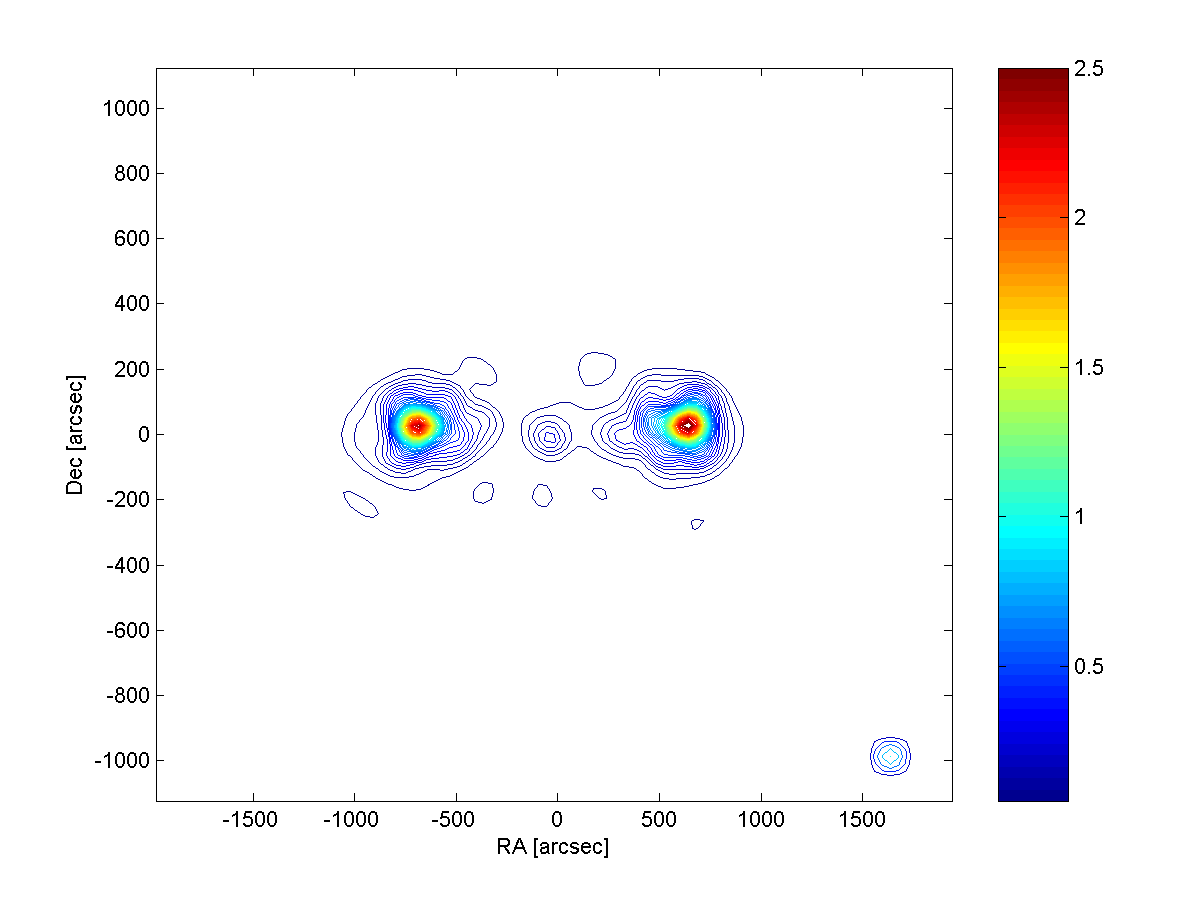
(c)	(d)

Figure 11: Reconstructed images of the CLEAN and LS-MVI algorithms. (a) CLEAN reconstructed image after 100 iterations. (b) CLEAN reconstructed image after 120 iterations. (c) LS-MVI reconstructed image after 100 iterations. (d) LS-MVI reconstructed image afer 300 iterations.

VII-B LOFAR Test Station Data

The LOFAR test station data were recorded using $25$ frequency bands of 156kHz using 45 antennas (array geometry is given in Figure (12 d)). The data were calibrated by S. Wijnholds. The AAR dirty image and the classic dirty image are given in Figure (12a) and (12b), respectively. Since the LOFAR station benefits from a good $(u,v)$ domain coverage, the two dirty images are similar. The reconstructed image using the LS-MVI algorithm is displayed in Figure (12 c); the spurious emission on the right side of the image was removed.

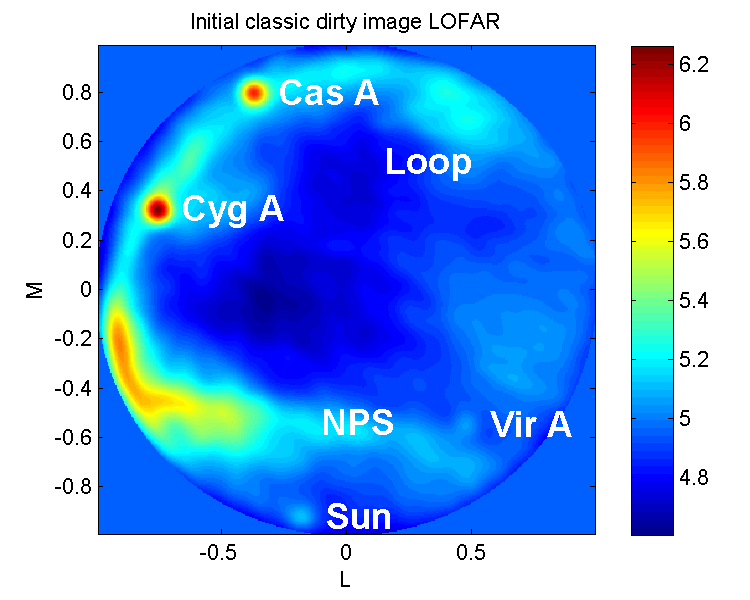
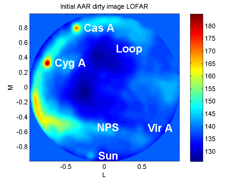
(a)	(b)
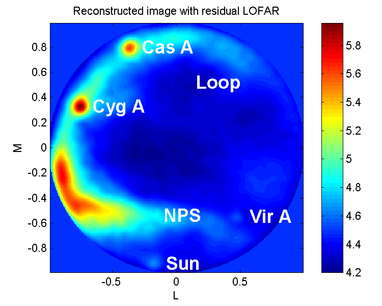
(c)	(d)

Figure 12: LOFAR station images. (a) classic dirty image. (b) AAR dirty image. (c) Reconstructed image using AAR based cleaning. (d) Array geometry

VII-C Abell 2256

The last example used VLA data of Abell 2256 The data measured by Clarke and Ensslin [56] contain a single frequency band around 1369 MHz. The data were processed using both CLEAN and LS-MVI algorithms for 30 iterations . We used a visibility domain CLEAN (updates were performed on the ungridded visibility). The initial data (dirty image) of the CLEAN are shown in Figure (13 a), The strong sidelobes structure is clearly visible as large circles in the dirty image. In contrast the initial AAR dirty image is shown in Figure (13 b). The sidelobes level is much lower and several point sources that are invisible in the classical dirty image are now visible. The reconstruction using the visibility domain CLEAN is shown in Figure (13 c). The sidelobes level is reduced and the source structure is clearly seen. The reconstruction using the LS-MVI algorithm is shown in Figure (13 d). Similar to the CLEAN, the sources structure is visible and the sidelobes level is significantly reduced. It should be emphasized that even though we have used only 30 iterations, the strong structure is consistent with that of [56] and [57].

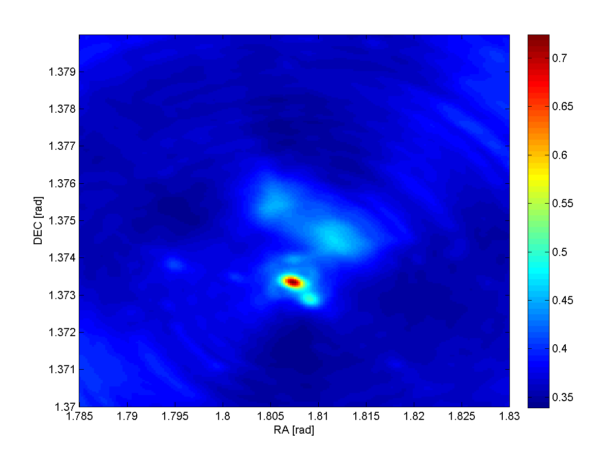
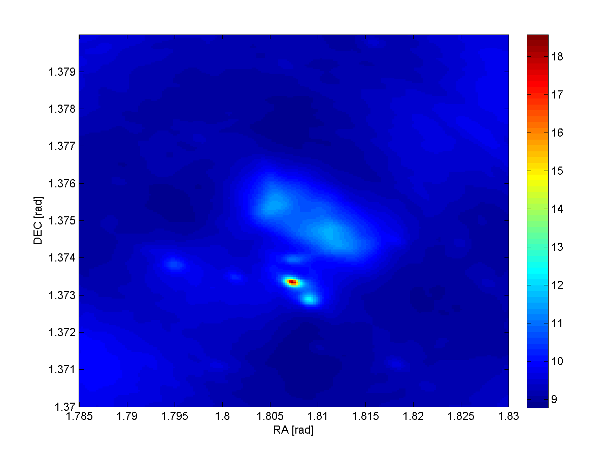
(a)	(b)
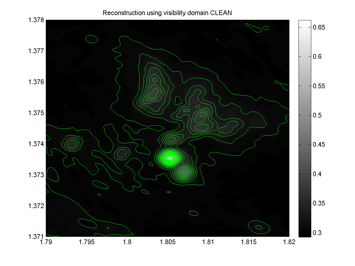
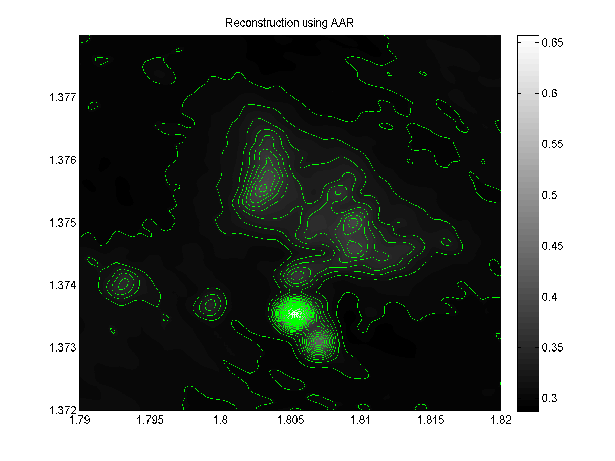
(c)	(d)

Figure 13: Abell 2256 images. (a) Initial classic dirty image. (b) Initial AAR dirty image. (c) classic CLEAN reconstructed image. (d) LS-MVI reconstructed image.

Authors

• Ronny Levanda received her B.Sc. in Physics and M.Sc. in neural networks, from the Tel Aviv University, in 1995 and 2000 respectively. She has 10 years of algorithm development experience, in High-Tec companies. She is now studying towards her Ph.D. in Bar-Ilan University.

• Amir Leshem Amir Leshem received the B.Sc. degree (cum laude) in mathematics and physics, the M.Sc. degree (cum laude) in mathematics, and the Ph.D. degree in mathematics, all from the Hebrew University, Jerusalem, Israel. He is one of the founders of the School of Electrical and Computer Engineering, Bar-Ilan University, Ramat Gan, Israel, where he is currently an Associate Professor and Head of the signal processing track. His main research interests include multichannel communication, applications of game theory to communication, array and statistical signal processing with applications to sensor arrays and networks, wireless communications, radio-astronomy, and brain research, set theory, logic, and foundations of mathematics.

References

- [1] K. Jansky, “Electrical disturbances apparently of extraterrestrial origin,” Proceedings of the IRE, vol. 21, pp. 1387–1398, Oct. 1933.
- [2] G. Reber, “Cosmic statics,” Proceedings of the IRE, vol. 28, pp. 68–70, Feb. 1940.
- [3] M. Ryle and D. Vonberg, “Solar radiation on 175 Mc./s,” Nature, vol. 158, pp. 339–340, Sept. 1946.
- [4] A. A. Penzias and R. W. Wilson, “A Measurement of Excess Antenna Temperature at 4080 Mc/s.,” Astrophysical Journal, vol. 142, pp. 419–421, July 1965.
- [5] F. G. Smoot and et al., “Structure in the COBE differential microwave radiometer first-year maps,” Astrophysical Journal Letters, vol. 396, pp. L1–L5, Sept. 1992.
- [6] A. Hewish, S. J. Bell, J. D. H. Pilkington, P. F. Scott, and R. A. Collins, “Observation of a rapidly pulsating radio source,” Nature, vol. 217, pp. 709–713, Feb. 1968.
- [7] H. Ewen and E. Purcell, “Observation of a line in the galactic radio spectrum,” Nature, vol. 168, p. 356, Feb. 1951.
- [8] R. A. Perley, J. W. Dreher, and J. J. Cowan, “The jet and filaments in Cygnus A,” Astrophysical Journal Letters, vol. 285, pp. L35–L38, Oct. 1984.
- [9] M. Ryle, “The new Cambridge radio telescope,” Nature, vol. 194, pp. 517–518, 1962.
- [10] J. A. Högbom, “Aperture synthesis with nonregular distribution of intereferometer baselines,” Astron. Astrophys. Suppl, vol. 15, pp. 417–426, 1974.
- [11] B. Frieden, “Restoring with maximum likelihood and maximum entropy,” Journal of the Optical Society of America, vol. 62, pp. 511–518, 1972.
- [12] S. Gull and G. Daniell, “Image reconstruction from incomplete and noisy data,” Nature, vol. 272, pp. 686–690, 1978.
- [13] J. Ables, “Maximum entropy spectreal analysis,” AAS, vol. 15, pp. 383–393, 1974.
- [14] S. Wernecke, “Two dimensional maximum entropy reconstruction of radio brightness,” Radio Science, vol. 12, pp. 831–844, 1977.
- [15] T. Cornwell and K. Evans, “A simple maximum entropy deconvolution algorithm,” Astronomy and Astrophysics, vol. 143, pp. 77–83, 1985.
- [16] U. Rau, S. Bhatnagar, M. Voronkov, and T. Cornwell, “Advances in calibration and imaging techniques in radio interferometry,” Proceeding of the IEEE, vol. 97, pp. 1472–1481, Aug 2009.
- [17] E. Pantin and J.-L. Starck, “Deconvolution of astronomical images using the multiscale maximum entropy method.,” Astronomy and Astrophysics Supplements, vol. 118, pp. 575–585, Sept. 1996.
- [18] D. S. Briggs, High fidelity deconvolution of moderately resolved sources. PhD thesis, The new Mexico Institute of Mining and Technology, Socorro, New Mexico, 1995.
- [19] A. Leshem and A. van der Veen, “Radio-astronomical imaging in the presence of strong radio interference,” IEEE Trans. on Information Theory, Special issue on information theoretic imaging, pp. 1730–1747, August 2000.
- [20] C. Ben-David and A. Leshem, “Parametric high resolution techniques for radio astronomical imaging,” Selected Topics in Signal Processing, IEEE Journal of, vol. 2, pp. 670–684, Oct. 2008.
- [21] R. Levanda and A. Leshem, “Radio astronomical image formation using sparse reconstruction techniques,” Electrical and Electronics Engineers in Israel, 2008. IEEEI 2008. IEEE 25th Convention of, pp. 716–720, Dec. 2008.
- [22] Y. Wiaux, L. Jacques, G. Puy, A. Scaife, and P. Vandergheynst, “Compressed sensing imaging techniques for radio interferometry,” Monthly Notices of The Royal Astonomical Society, Submitted 2009.
- [23] R. Reid, “Smear fitting: a new image-deconvolution method for interferometric data,” Monthly Notices of the Royal Astronomical Society, vol. 367, no. 4, pp. 1766–1780, 2006.
- [24] A. Thompson, J. Moran, and G. Swenson, eds., Interferometry and Synthesis in Radio astronomy. John Wiley and Sons, 1986.
- [25] G. Taylor, C. Carilli, and R. Perley, Synthesis Imaging in Radio-Astronomy. Astronomical Society of the Pacific, 1999.
- [26] A. Leshem, A. van der Veen, and A. J. Boonstra, “Multichannel interference mitigation techniques in radio-astronomy,” The Astrophysical Journal Supplements, pp. 355–373, November 2000.
- [27] S. van der Tol, Bayesian Estimation for Ionospheric Calibration in Radio Astronomy. PhD thesis, Delft University of Technology, 2009.
- [28] R. N. S. Wijnholds, S. van der Tol and A.-J. van der Veen, “Calibration challenges for next generation of radio telescopes,” IEEE Signal Processing magazine, Submitted 2009.
- [29] T. Cornwell, “Multiscale CLEAN deconvolution of radio synthesis images,” Selected Topics in Signal Processing, IEEE Journal of, vol. 2, pp. 793–801, Oct. 2008.
- [30] B. G. Clark, “An efficient implementation of the algorithm ”clean”,” Astronomy and Astrophysics, vol. 89, pp. 377–378, 1980.
- [31] F. R. Schwab, “Relaxing the isoplanatism assumption in self-calibration; applications to low-frequency radio interfetomerty,” The Astronomical Journal, vol. 89, pp. 1076–1081, July 1984.
- [32] W. D. Cotton and J. M. Uson, “Pixelization and dynamic range in radio interferometry,” Astronomy and Astrophysics, vol. 490, pp. 455–460, Oct. 2008.
- [33] M. A. Voronkov and M. H. Wieringa, “”the cotton-schwab clean at ultra-high dynamic range”,” Experimental Astronomy, vol. 18, pp. 13–29, apr 2004.
- [34] T. Cornwell, K. Golap, and S. Bhatnagar, “The non-coplanar baselines effect in radio interferometry: The w-projetion algorithm,” IEEE Journal of Selected Topics in Signal Processing, vol. 2, pp. 647–657, October 2008.
- [35] R. H. Frater and I. S. Docherty, “On the reduction of three dimensional interferometer measurements,” Astrononomy and Astrophysics, vol. 84, pp. 75–77, Apr. 1980.
- [36] S. Bhatnager and T. Cornwell, “Adaptive scale sensitive deconvolution of interferometric images I. Adaptive scale pixel (asp) decomposition,” Astronomy and Astrophysics, vol. 426, pp. 747–754, 2004.
- [37] E. Jaynes, “Information theory and statistical mechanics,” Physics Review, vol. 106, pp. 620–630, May 1957.
- [38] E. T. Jaynes, “On the rational of maximum-entropy methods,” Proceedings of the IEEE, vol. 70, pp. 939–952, sep 1982.
- [39] J. Roberts, ed., Indirect imaging. Cambridge university press, 1984.
- [40] R. Narayan and R. Nityananda, “Maximum entropy image restoration in astronomy,” Annual review of of Astronomy and Astrophysics, vol. 24, pp. 127–170, 1986.
- [41] R. Sault, “A modification of the Cornwell and Evans maximum entropy algorithm,” The Astrophysical Journal, vol. 354, pp. L61–63, 1990.
- [42] J. Skilling and R. Bryan”, “maximum entropy image restoration algorithm,” Monthly Notices of the Royal Astronomical Society, vol. 211, pp. 111–124, 1984.
- [43] K. Maisinger, M. P. Hobson, and A. N. Lasenby, “Maximum-entropy image reconstruction using wavelets,” Monthly Notices of the Royal Astronomical Society, vol. 347, pp. 339–354, Jan. 2004.
- [44] K. Marsh and J. Richardson, “The objective function implicit in the CLEAN algorithm,” Astronomy and Astrophysics (ISSN 0004-6361), vol. 182, pp. 174–178, Aug 1987.
- [45] D. Dobson and F. Santosa, “Recovery of blocky images from noisy and blurred data,” SIAM Journal on Applied Mathematics, vol. 56, no. 4, pp. 1181–1198, 1996.
- [46] S. Chen, D. Donoho, and M. Saunders, “Atomic decomposition by basis pursuit,” Siam J. Sci Comput, vol. 20, no. 1, pp. 33–61, 1998.
- [47] A. Feuer and A. Nemirovski, “On sparse representation in pairs of bases,” IEEE trasactions on information theory, vol. 49, pp. 1579–1581, June 2003.
- [48] M. Elad and A. Bruckstein, “A generalized uncertainty principle and sparse representation in pairs of bases,” IEEE trasactions on information theory.
- [49] M. Rudelson and R. Vershynim, “Sparse reconstruction by convex relaxation: Fourier and gaussian measurements,” Mar 2006.
- [50] A. van der Veen, A. Leshem, and A. Boonstra, “Array signal processing in radio-astronomy,” Experimental Astronomy, vol. 17, pp. 231–249, June 2004.
- [51] P. Stoica, Z. Wang, and J. Li, “Robust Capon beamforming,” IEEE Signal Processing Letters, vol. 10, pp. 172–175, Jun. 2003.
- [52] L. Vandenberghe and S. Boyd, “Semidefinite programming,” SIAM Review, vol. 38, pp. 49–95, Mar. 1996.
- [53] T. Pearson and A. Readhead, “Image formation by self-calibration in radio astronomy,” Annual Rev. Astronomy and Astrophysics, vol. 22, pp. 97–130, 1984.
- [54] J. Li, P. Stoica, and Z. Wang, “Doubly constrained robust Capon beamformer,” IEEE Transactions on Signal Processing, vol. 52, pp. 2407–2423, Sept. 2004.
- [55] H. Rottgering, I. Snellen, G. Miley, J. P. de Jong, R. J. Hanisch, and R. Perley, “VLA observations of the rich X-ray cluster Abell 2256,” Astrophysical Journal, vol. 436, pp. 654–668, Dec. 1994.
- [56] T. Clarke and T. Ensslin, “Deep 1.4 GHz very large array observations of the radio halo and relic in Abell 2256,” The Astronomical Journal, vol. 131, pp. 2900–2912, June 2006.
- [57] A. H. Bridle and E. B. Fomalont, “Complex radio emission from the X-ray cluster Abell 2256,” Astronomy and Astrophysics, vol. 52, pp. 107–113, Oct. 1976.