Stochastic Control Complexity and Stochastic Synchronization in Coupled Map Lattices and Cellular Automata Spain Juan R. Sánchez Universidad Nacional de Mar del Plata Argentine

1 Introduction

Nowadays the question ‘what is complexity?’ is a challenge to be answered. This question is triggering a great quantity of works in the frontier of physics, biology, mathematics and computer science. Even more when this century has been told to be the century of complexity (Hawking,, 2000). Although there seems to be no urgency to answer the above question, many different proposals that have been developed to this respect can be found in the literature (Perakh,, 2004). In this context, several articles concerning statistical complexity and stochastic processes are collected in this chapter.

Complex patterns generated by the time evolution of a one-dimensional digitalized coupled map lattice are quantitatively analyzed in Section 2. A method for discerning complexity among the different patterns is implemented. The quantitative results indicate two zones in parameter space where the dynamics shows the most complex patterns. These zones are located on the two edges of an absorbent region where the system displays spatio-temporal intermittency.

The synchronization of two stochastically coupled one-dimensional cellular automata (CA) is analyzed in Section 3. It is shown that the transition to synchronization is characterized by a dramatic increase of the statistical complexity of the patterns generated by the difference automaton. This singular behavior is verified to be present in several CA rules displaying complex behavior.

In Sections 4 and 5, we are concerned with the stability analysis of patterns in extended systems. In general, it has been revealed to be a difficult task. The many nonlinearly interacting degrees of freedom can destabilize the system by adding small perturbations to some of them. The impossibility to control all those degrees of freedom finally drives the dynamics toward a complex spatio-temporal evolution. Hence, it is of a great interest to develop techniques able to compel the dynamics toward a particular kind of structure. The application of such techniques forces the system to approach the stable manifold of the required pattern, and then the dynamics finally decays to that target pattern.

Synchronization strategies in extended systems can be useful in order to achieve such goal. In Section 4, we implement stochastic synchronization between the present configurations of a cellular automata and its precedent ones in order to search for constant patterns. In Section 5, this type of synchronization is specifically used to find symmetrical patterns in the evolution of a single automaton.

2 Complexity in Two-Dimensional Patterns Generated by Coupled Map Lattices

It should be kept in mind that in ancient epochs, time, space, mass, velocity, charge, color, etc. were only perceptions. In the process they are becoming concepts, different tools and instruments are invented for quantifying the perceptions. Finally, only with numbers the scientific laws emerge. In this sense, if by complexity it is to be understood that property present in all systems attached under the epigraph of ‘complex systems’, this property should be reasonably quantified by the different measures that were proposed in the last years. This kind of indicators is found in those fields where the concept of information is crucial. Thus, the effective measure of complexity (Grassberger,, 1986) and the thermodynamical depth (Lloyd & Pagels,, 1988) come from physics and other attempts such as algorithmic complexity (Kolmogorov,, 1965; Chaitin,, 1966), Lempel-Ziv complexity (Lempel & Ziv,, 1976) and $\epsilon$-machine complexity (Cruthfield,, 1989) arise from the field of computational sciences.

In particular, taking into account the statistical properties of a system, an indicator called the LMC (LópezRuiz-Mancini-Calbet) complexity has been introduced (Lopez-Ruiz,, 1994; Lopez-Ruiz et al.,, 1995). This magnitude identifies the entropy or information stored in a system and its disequilibrium i.e., the distance from its actual state to the probability distribution of equilibrium, as the two basic ingredients for calculating its complexity. If $H$ denotes the information stored in the system and $D$ is its disequilibrium, the LMC complexity $C$ is given by the formula:

$$C(\bar{p})=H(\bar{p})\cdot D(\bar{p})\;=$$

$$=-k\left(\sum_{i=1}^{N}p_{i}\log p_{i}\right)\cdot\left(\sum_{i=1}^{N}\,\left(p_{i}-\frac{1}{N}\right)^{2}\right)\,$$ (1)

where $\bar{p}=\{p_{i}\}$, with $p_{i}\geq 0$ and $i=1,\cdots,N$, represents the distribution of the $N$ accessible states to the system, and $k$ is a constant taken as $1/\log N$.

As well as the Euclidean distance $D$ is present in the original LMC complexity, other kinds of disequilibrium measures have been proposed in order to remedy some statistical characteristics considered troublesome for some authors (Feldman & Crutchfield,, 1998). In particular, some attention has been focused (Lin,, 1991; Martin et al.,, 2003) on the Jensen-Shannon divergence $D_{JS}$ as a measure for evaluating the distance between two different distributions $(\bar{p}_{1},\bar{p}_{2})$. This distance reads:

$$D_{JS}(\bar{p}_{1},\bar{p}_{2})=H(\pi_{1}\bar{p}_{1}+\pi_{2}\bar{p}_{2})-\pi_{1}H(\bar{p}_{1})-\pi_{2}H(\bar{p}_{2}),$$ (2)

with $\pi_{1},\pi_{2}$ the weights of the two probability distributions $(\bar{p}_{1},\bar{p}_{2})$ verifying $\pi_{1},\pi_{2}\geq 0$ and $\pi_{1}+\pi_{2}=1$. The ensuing statistical complexity

$$C_{JS}=H\cdot D_{JS}$$ (3)

becomes intensive and also keeps the property of distinguishing among distinct degrees of periodicity (Lamberti et al.,, 2004). Here, we consider $\bar{p}_{2}$ the equiprobability distribution and $\pi_{1}=\pi_{2}=0.5$.

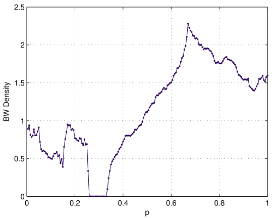
Figure 1: $\beta$ versus $p$. The $\beta$-statistics (or BW density) for each $p$ is the rate between the number of black and white cells depicted by the system in the two-dimensional representation of its after-transient time evolution. (Computations have been performed with $\Delta p=0.005$ for a lattice of $10000$ sites after a transient of $5000$ iterations and a running of other $2000$ iterations).

As it can be straightforwardly seen, all these LMC-like complexities vanish both for completely ordered and for completely random systems as it is required for the correct asymptotic properties of a such well-behaved measure. Recently, they have been successfully used to discern situations regarded as complex in discrete systems out of equilibrium (Shiner et al.,, 1999; Calbet & Lopez-Ruiz,, 2001; Yu & Chen,, 2000; Rosso et al.,, 2003, 2005; Lovallo et al.,, 2005).

As an example, the local transition to chaos via intermittency (Pomeau & Manneville,, 1980) in the logistic map, $x_{n+1}=\lambda x_{n}(1-x_{n})$ presents a sharp transition when C is plotted versus the parameter $\lambda$ in the region around the instability for $\lambda\sim\lambda_{t}=3.8284$. When $\lambda<\lambda_{t}$ the system approaches the laminar regime and the bursts become more unpredictable. The complexity increases. When the point $\lambda=\lambda_{t}$ is reached a drop to zero occurs for the magnitude $C$. The system is now periodic and it has lost its complexity. The dynamical behavior of the system is finally well reflected in the magnitude $C$ (see (Lopez-Ruiz et al.,, 1995)).

When a one-dimensional array of such maps is put together a more complex behavior can be obtained depending on the coupling among the units. Ergo the phenomenon called spatio-temporal intermittency can emerge (Chate & Manneville,, 1987; Houlrik,, 1990; Rolf et al.,, 1998). This dynamical regime corresponds with a situation where each unit is weakly oscillating around a laminar state that is aperiodically and strongly perturbed for a traveling burst. In this case, the plot of the one-dimensional lattice evolving in time gives rise to complex patterns on the plane. If the coupling among units is modified the system can settle down in an absorbing phase where its dynamics is trivial (Argentina & Coullet,, 1997; Zimmermann et al.,, 2000) and then homogeneous patterns are obtained. Therefore an abrupt transition to spatio-temporal intermittency can be depicted by the system (Pomeau,, 1986; Menon et al.,, 2003) when modifying the coupling parameter.

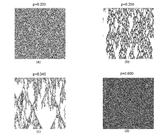
Figure 2: Digitalized plot of the one-dimensional coupled map lattice (axe OX) evolving in time (axe OY) according to Eq. (4): if $x_{i}^{n}>0.5$ the $(i,n)$-cell is put in white color and if $x_{i}^{n}<0.5$ the $(i,n)$-cell is put in black color. The discrete time $n$ is reset to zero after the transitory. (Lattices of $300\times 300$ sites, i.e., $0<i<300$ and $0<n<300$).

In this section, we are concerned with measuring $C$ and $C_{JS}$ in a such transition for a coupled map lattice of logistic type (Sanchez & Lopez-Ruiz, 2005-a, ). Our system will be a line of sites, $i=1,\ldots,L$, with periodic boundary conditions. In each site $i$ a local variable $x_{i}^{n}$ evolves in time ($n$) according to a discrete logistic equation. The interaction with the nearest neighbors takes place via a multiplicative coupling:

$$x_{i}^{n+1}=(4-3pX_{i}^{n})x_{i}^{n}(1-x_{i}^{n}),$$ (4)

where $p$ is the parameter of the system measuring the strength of the coupling ($0<p<1$). The variable $X_{i}^{n}$ is the digitalized local mean field,

$$X_{i}^{n}=nint\left[\frac{1}{2}\>({x_{i+1}^{n}+x_{i-1}^{n}})\right]\>,$$ (5)

with $nint(.)$ the integer function rounding its argument to the nearest integer. Hence $X_{i}^{n}=0$ or $1$.

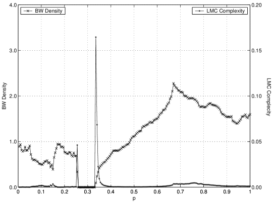
Figure 3: ($\bullet$) $C$ versus $p$. Observe the peaks of the LMC complexity located just on the borders of the absorbent region $0.258<p<0.335$, where $\beta=0$ ($\times$). (Computations have been performed with $\Delta p=0.005$ for a lattice of $10000$ sites after a transient of $5000$ iterations and a running of other $2000$ iterations).

There is a biological motivation behind this kind of systems (Lopez-Ruiz & Fournier-Prunaret,, 2004; Lopez-Ruiz,, 2005). It could represent a colony of interacting competitive individuals. They evolve randomly when they are independent ($p=0$). If some competitive interaction ($p>0$) among them takes place the local dynamics loses its erratic component and becomes chaotic or periodic in time depending on how populated the vicinity is. Hence, for bigger $X_{i}^{n}$ more populated is the neighborhood of the individual $i$ and more constrained is its free action. At a first sight, it would seem that some particular values of $p$ could stabilize the system. In fact, this is the case. Let us choose a number of individuals for the colony ($L=500$ for instance), let us initialize it randomly in the range $0<x_{i}<1$ and let it evolve until the asymptotic regime is attained. Then the black/white statistics of the system is performed. That is, the state of the variable $x_{i}$ is compared with the critical level $0.5$ for $i=1,\ldots,L$: if $x_{i}>0.5$ the site $i$ is considered white (high density cell) and a counter $N_{w}$ is increased by one, or if $x_{i}<0.5$ the site $i$ is considered black (low density cell) and a counter $N_{b}$ is increased by one. This process is executed in the stationary regime for a set of iterations. The black/white statistics is then the rate $\beta=N_{b}/N_{w}$. If $\beta$ is plotted versus the coupling parameter $p$ the Figure 1 is obtained.

The region $0.258<p<0.335$ where $\beta$ vanishes is remarkable. As stated above, $\beta$ represents the rate between the number of black cells and the number of white cells appearing in the two-dimensional digitalized representation of the colony evolution. A whole white pattern is obtained for this range of $p$. The phenomenon of spatio-temporal intermittency is displayed by the system in the two borders of this parameter region (Fig. 2). Bursts of low density (black color) travel in an irregular way through the high density regions (white color). In this case two-dimensional complex patterns are shown by the time evolution of the system (Fig. 2b-c). If the coupling $p$ is far enough from this region, i.e., $p<0.25$ or $p>0.4$, the absorbent region loses its influence on the global dynamics and less structured and more random patterns than before are obtained (Fig. 2a-d). For $p=0$ we have no coupling of the maps, and each map generates so called fully developed chaos, where the invariant measure is well-known to be symmetric around $0.5$. From this we conclude that $\beta(p=0)=1$. Let us observe that this symmetrical behavior of the invariant measure is broken for small $p$, and $\beta$ decreases slightly in the vicinity of $p=0$.

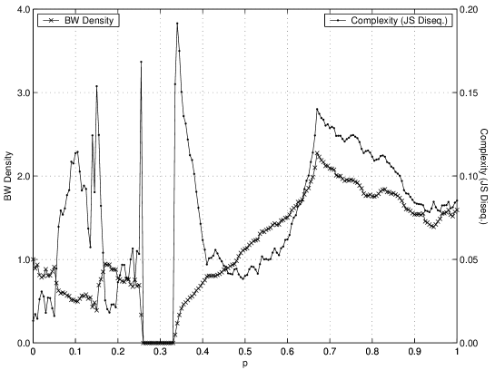
Figure 4: ($\cdot$) $C_{JS}$ versus $p$. The peaks of this modified LMC complexity are also evident just on the borders of the absorbent region $0.258<p<0.335$, where $\beta=0$ ($\times$). (Computations have been performed with $\Delta p=0.005$ for a lattice of $10000$ sites after a transient of $5000$ iterations and a running of other $2000$ iterations).

If the LMC complexities are quantified as function of $p$, our intuition is confirmed. The method proposed in (Lopez-Ruiz et al.,, 1995) to calculate $C$ is now adapted to the case of two-dimensional patterns. First, we let the system evolve until the asymptotic regime is attained. This transient is discarded. Then, for each time $n$, we map the whole lattice in a binary sequence: $0$ if $x_{i}^{n}<0.5$ and $1$ if $x_{i}^{n}>0.5$, for $i=1,\ldots,L$. This $L$-binary string is analyzed by blocks of $n_{o}$ bits, where $n_{o}$ can be considered the scale of observation. For this scale, there are $2^{n_{o}}$ possible states but only some of them are accessible. These accessible states as well as their probabilities are found in the $L$-binary string. Next, the magnitudes $H$, $D$, $D_{JS}$, $C$ and $C_{JS}$ are directly calculated for this particular time $n$ by applying the formulas (1-3). We repeat this process for a set of successive time units $(n,n+1,\cdots,n+m)$. The mean values of $H$, $D$, $D_{JS}$, $C$ and $C_{JS}$ for these $m$ time units are finally obtained and plotted in Fig. 3-4.

Figures 3,4 show the result for the case of $n_{o}=10$. Let us observe that the highest $C$ and $C_{JS}$ are reached when the dynamics displays spatio-temporal intermittency, that is, the most complex patterns are obtained for those values of $p$ that are located on the borders of the absorbent region $0.258<p<0.335$. Thus the plot of $C$ and $C_{JS}$ versus $p$ shows two tight peaks around the values $p=0.256$ and $p=0.34$ (Fig. 3,4). Let us remark that the LMC complexity $C$ can be neglected far from the absorbent region. Contrarily to this behavior, the magnitude $C_{JS}$ also shows high peaks in some other sharp transition of $\beta$ located in the region $0<p<25$, and an intriguing correlation with the black/white statistics in the region $0.4<p<1$. All these facts as well as the stability study of the different dynamical regions of system (4) are not the object of the present writing but they deserve attention and a further study.

If the detection of complexity in the two-dimensional case requires to identify some sharp change when comparing different patterns, those regions in the parameter space where an abrupt transition happens should be explored in order to obtain the most complex patterns. Smoothness seems not to be at the origin of complexity. As well as a selected few distinct molecules among all the possible are in the basis of life (McKay,, 2004), discreteness and its spiky appearance could indicate the way towards complexity. Let us recall that the distributions with the highest LMC complexity are just those distributions with a spiky-like appearance (Calbet & Lopez-Ruiz,, 2001; Anteneodo & Plastino,, 1996). In this line, the striking result here exposed confirms the capability of the LMC-like complexities for signaling a transition to complex behavior when regarding two-dimensional patterns (Sanchez & Lopez-Ruiz, 2005-b, ).

3 Detecting Synchronization in Cellular Automata by Complexity Measurements

Despite all the efforts devoted to understand the meaning of complexity, we still do not have an instrument in the laboratories specially designed for quantifying this property. Maybe this is not the final objective of all those theoretical attempts carried out in the most diverse fields of knowledge in the last years (Kolmogorov,, 1965; Chaitin,, 1966; Lempel & Ziv,, 1976; Bennett,, 1985; Grassberger,, 1986; Lloyd & Pagels,, 1988; Cruthfield,, 1989; Shiner et al.,, 1999), but, for a moment, let us think in that possibility.

Similarly to any other device, our hypothetical apparatus will have an input and an output. The input could be the time evolution of some variables of the system. The instrument records those signals, analyzes them with a proper program and finally screens the result in the form of a complexity measurement. This process is repeated for several values of the parameters controlling the dynamics of the system. If our interest is focused in the most complex configuration of the system we have now the possibility of tuning such an state by regarding the complexity plot obtained at the end of this process.

As a real applicability of this proposal, let us apply it to an à-la-mode problem. The clusterization or synchronization of chaotic coupled elements was put in evidence at the beginning of the nineties (Kaneko,, 1989; Lopez-Ruiz & Perez-Garcia,, 1991). Since then, a lot of publications have been devoted to this subject (Boccaletti et al.,, 2002). Let us consider one particular of these systems to illuminate our proposal.

(1) SYSTEM: We take two coupled elementary one dimensional cellular automata (CA: see next section in which CA are concisely explained) displaying complex spatio-temporal dynamics (Wolfram,, 1983). It has been shown that this system can undergo through a synchronization transition (Morelli & Zanette,, 1998). The transition to full synchronization occurs at a critical value $p_{c}$ of a synchronization parameter $p$. Briefly the numerical experiment is as follows. Two $L$-cell CA with the same evolution rule $\Phi$ are started from different random initial conditions for each automaton. Then, at each time step, the dynamics of the coupled CA is governed by the successive application of two evolution operators; the independent evolution of each CA according to its corresponding rule $\Phi$ and the application of a stochastic operator that compares the states $\sigma_{i}^{1}$ and $\sigma_{i}^{2}$ of all the cells, $i=1,...L$, in each automaton. If $\sigma_{i}^{1}=\sigma_{i}^{2}$, both states are kept invariant. If $\sigma_{i}^{1}\neq\sigma_{i}^{2}$, they are left unchanged with probability $1-p$, but both states are updated either to $\sigma_{i}^{1}$ or to $\sigma_{i}^{2}$ with equal probability $p/2$. It is shown in reference (Morelli & Zanette,, 1998) that there exists a critical value of the synchronization parameter ($p_{c}=0.193$ for the rule $18$) above for which full synchronization is achieved.

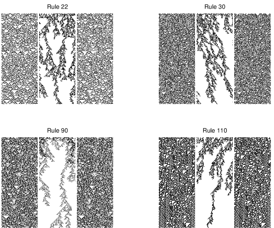
Figure 5: Spatio-temporal patterns just above the synchronization transition. The left and the right plots show $250$ successive states of the two coupled automata and the central plot is the corresponding difference automaton for the rules $22$, $30$, $90$ and $110$. The number of sites is $L=100$ and the coupling probability is $p=0.23$.

(2) DEVICE: We choose a particular instrument to perform our measurements, that is capable of displaying the value of the LMC complexity ($C$) (Lopez-Ruiz et al.,, 1995) defined as in Eq. (1), $C(\{\rho_{i}\})=H(\{\rho_{i}\})\cdot D(\{\rho_{i}\})\;$, where $\{\rho_{i}\}$ represents the set of probabilities of the $N$ accessible discrete states of the system, with $\rho_{i}\geq 0$ , $i=1,\cdots,N$, and $k$ is a constant. If $k=1/logN$ then we have the normalized complexity. $C$ is a statistical measure of complexity that identifies the entropy or information stored in a system and its disequilibrium, i.e., the distance from its actual state to the probability distribution of equilibrium, as the two basic ingredients for calculating the complexity of a system. This quantity vanishes both for completely ordered and for completely random systems giving then the correct asymptotic properties required for a such well-behaved measure, and its calculation has been useful to successfully discern many situations regarded as complex.

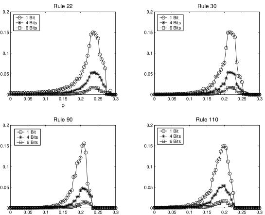
Figure 6: The normalized complexity $C$ versus the coupling probability $p$ for different scales of observation: $n_{o}=1$ ($\circ$),$n_{o}=4$ ($\star$) and $n_{o}=6$ ($\Box$). $C$ has been calculated over the last $300$ iterations of a running of $600$ of them for a lattice with $L=1000$ sites. The synchronization transition is clearly depicted around $p\approx 0.2$ for the different rules.

(3) INPUT: In particular, the evolution of two coupled CA evolving under the rules $22$, $30$, $90$ and $110$ is analyzed. The pattern of the difference automaton will be the input of our device. In Fig. 5 it is shown for a coupling probability $p=0.23$, just above the synchronization transition. The left and the right plots show $250$ successive states of the two automata, whereas the central plot displays the corresponding difference automaton. Such automaton is constructed by comparing one by one all the sites ($L=100$) of both automata and putting zero when the states $\sigma_{i}^{1}$ and $\sigma_{i}^{2}$, $i=1\ldots L$, are equal or putting one otherwise. It is worth to observe that the difference automaton shows an interesting complex structure close to the synchronization transition. This complex pattern is only found in this region of parameter space. When the system if fully synchronized the difference automaton is composed by zeros in all the sites, while when there is no synchronization at all the structure of the difference automaton is completely random.

(4) METHOD OF MEASUREMENT: How to perform the measurement of $C$ for such two-dimensional patterns has been presented in the former section (Sanchez & Lopez-Ruiz, 2005-a, ). We let the system evolve until the asymptotic regime is attained. The variable $\sigma_{i}^{d}$ in each cell of the difference pattern is successively translated to an unique binary sequence when the variable $i$ covers the spatial dimension of the lattice, $i=1,\ldots,L$, and the time variable $n$ is consecutively increased. This binary string is analyzed in blocks of $n_{o}$ bits, where $n_{o}$ can be considered the scale of observation. The accessible states to the system among the $2^{n_{o}}$ possible states is found as well as their probabilities. Then, the magnitudes $H$, $D$ and $C$ are directly calculated and screened by the device.

(5) OUTPUT: The results of the measurement are shown in Fig. 6. The normalized complexity $C$ as a function of the synchronization parameter $p$ is plotted for different coupled one-dimensional CA that evolve under the rules $22$, $30$, $90$ and $110$ , which are known to generate complex patterns. All the plots of Fig. 6 were obtained using the following parameters: number of cell of the automata, $L=1000$; total evolution time, $T=600$ steps. For all the cases and scales analyzed, the statistical complexity $C$ shows a dramatic increase close to the synchronization transition. It reflects the complex structure of the difference automaton and the capability of the measurement device here proposed for clearly signaling the synchronization transition of two coupled CA.

These results are in agreement with the measurements of $C$ performed in the patterns generated by a one-dimensional logistic coupled map lattice in the former section (Sanchez & Lopez-Ruiz, 2005-a, ). There the LMC statistical complexity ($C$) also shows a singular behavior close to the two edges of an absorbent region where the lattice displays spatio-temporal intermittency. Hence, in our present case, the synchronization region of the coupled systems can be interpreted as an absorbent region of the difference system. In fact, the highest complexity is reached on the border of this region for $p\approx 0.2$. The parallelism between both systems is therefore complete.

4 Self-Synchronization of Cellular Automata

Cellular automata (CA) are discrete dynamical systems, discrete both in space and time. The simplest one dimensional version of a cellular automaton is formed by a lattice of $N$ sites or cells, numbered by an index $i=1,\ldots,N$, and with periodic boundary conditions. In each site, a local variable $\sigma_{i}$ taking a binary value, either $0$ or $1$, is asigned. The binary string $\sigma(t)$ formed by all sites values at time $t$ represents a configuration of the system. The system evolves in time by the application of a rule $\Phi$. A new configuration $\sigma(t+1)$ is obtained under the action of the rule $\Phi$ on the state $\sigma(t)$. Then, the evolution of the automata can be writen as

$$\sigma(t+1)=\Phi\>[\sigma(t)].$$ (6)

If coupling among nearest neighbors is used, the value of the site $i$, $\sigma_{i}(t+1)$, at time $t+1$ is a function of the value of the site itself at time $t$, $\sigma_{i}(t)$, and the values of its neighbors $\sigma_{i-1}(t)$ and $\sigma_{i+1}(t)$ at the same time. Then, the local evolution is expressed as

$$\sigma_{i}(t+1)=\phi(\sigma_{i-1}(t),\sigma_{i}(t),\sigma_{i+1}(t)),$$ (7)

being $\phi$ a particular realization of the rule $\Phi$. For such particular implementation, there will be $2^{3}$ different local input configurations for each site and, for each one of them, a binary value can be assigned as output. Therefore there will be $2^{8}$ different rules $\phi$, also called the Wolfram rules. Each one of these rules produces a different dynamical evolution. In fact, dynamical behavior generated by all $256$ rules were already classified in four generic classes. The reader interested in the details of such classification is addressed to the original reference (Wolfram,, 1983).

CA provide us with simple dynamical systems, in which we would like to essay different methods of synchronization. A stochastic synchronization technique was introduced in (Morelli & Zanette,, 1998) that works in synchronizing two CA evolving under the same rule $\Phi$. The two CA are started from different initial conditions and they are supposed to have partial knowledge about each other. In particular, the CA configurations, $\sigma^{1}(t)$ and $\sigma^{2}(t)$, are compared at each time step. Then, a fraction $p$ of the total different sites are made equal (synchronized). The synchronization is stochastic since the location of the sites that are going to be equal is decided at random. Hence, the dynamics of the two coupled CA, $\sigma(t)=(\sigma^{1}(t),\sigma^{2}(t))$, is driven by the successive application of two operators:

1. the deterministic operator given by the CA evolution rule $\Phi$, $\Phi[\sigma(t)]=(\Phi[\sigma^{1}(t)],\Phi[\sigma^{2}(t)])$, and

2. the stochastic operator $\Gamma_{p}$ that produces the result $\Gamma_{p}[\sigma(t)]$, in such way that, if the sites are different ($\sigma_{i}^{1}\neq\sigma_{i}^{2}$), then $\Gamma_{p}$ sets both sites equal to $\sigma_{i}^{1}$ with the probability $p/2$ or equal to $\sigma_{i}^{2}$ with the same probability $p/2$. In any other case $\Gamma_{p}$ leaves the sites unchanged.

Therefore the temporal evolution of the system can be written as

$$\sigma(t+1)=(\Gamma_{p}\circ\Phi)[\sigma(t)]=\Gamma_{p}[(\Phi[\sigma^{1}(t)],\Phi[\sigma^{2}(t)])].$$ (8)

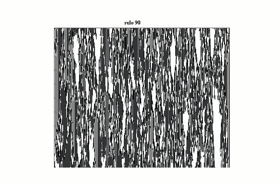
Figure 7: Rule $90$ has two stable patterns: one repeats the $011$ string and the other one the $00$ string. Such patterns are reached by the first self-synchronization method but there is a dynamical competition between them. In this case $p=0{.}9$. Binary value $0$ is represented in white and $1$ in black. Time goes from top to bottom.

A simple way to visualize the transition to synchrony can be done by displaying the evolution of the difference automaton (DA),

$$\delta_{i}(t)=\mid\sigma_{i}^{1}(t)-\sigma_{i}^{2}(t)\mid.$$ (9)

The mean density of active sites for the DA

$$\rho(t)={1\over N}\sum_{i=1}^{N}\delta_{i}(t),$$ (10)

represents the Hamming distance between the automata and verifies $0\leq\rho\leq 1$. The automata will be synchronized when $\lim_{t\rightarrow\infty}\rho(t)=0$. As it has been described in (Morelli & Zanette,, 1998) that two different dynamical regimes, controlled by the parameter $p$, can be found in the system behavior:

$$p<p_{c} \rightarrow \>\lim_{t\rightarrow\infty}\rho(t)\neq 0$$ (no synchronization),

$$p>p_{c} \rightarrow \hbox{$\>\lim_{t\rightarrow\infty}\rho(t)=0$ (synchronization)},$$

being $p_{c}$ the parameter for which the transition to the synchrony occurs. When $p\lesssim p_{c}$ complex structures can be observed in the DA time evolution. In Fig. 5, typical cases of such behavior are shown near the synchronization transition. Lateral panels represent both CA evolving in time where the central strip displays the evolution of the corresponding DA. When $p$ comes close to the critical value $p_{c}$ the evolution of $\delta(t)$ becomes rare and resembles the problem of structures trying to percolate in the plane (Pomeau,, 1986). A method to detect this kind of transition, based in the calculation of a statistical measure of complexity for patterns, has been proposed in the former sections (Sanchez & Lopez-Ruiz, 2005-a, ), (Sanchez & Lopez-Ruiz, 2005-b, ).

4.1 First Self-Synchronization Method

Let us now take a single cellular automaton (Toffoli & Margolus,, 1987; Ilachinski,, 2001). If $\sigma^{1}(t)$ is the state of the automaton at time t, $\sigma^{1}(t)=\sigma(t)$, and $\sigma^{2}(t)$ is the state obtained from the application of the rule $\Phi$ on that state, $\sigma^{2}(t)=\Phi[\sigma^{1}(t)]$, then the operator $\Gamma_{p}$ can be applied on the pair $(\sigma^{1}(t),\sigma^{2}(t))$, giving rise to the evolution law

$$\sigma(t+1)=\Gamma_{p}[(\sigma^{1}(t),\sigma^{2}(t))]=\Gamma_{p}[(\sigma(t),\Phi[\sigma(t)])].$$ (11)

The application of the $\Gamma_{p}$ operator is as follows. When $\sigma_{i}^{1}\neq\sigma_{i}^{2}$, the sites $i$ of the state $\sigma^{2}(t)$ are updated to the correspondent values taken in $\sigma^{1}(t)$ with a probability $p$. The updated array $\sigma^{2}(t)$ is the new state $\sigma(t+1)$.

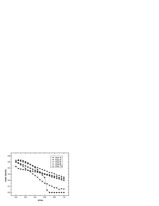
Figure 8: Mean density $\rho$ vs. $pmax=\tilde{p}$ for different rules evolving under the second synchronization method. The existence of a transition to a synchronized state can be clearly observed for rule $18$.

It is worth to observe that if the system is initialized with a configuration constant in time for the rule $\Phi$, $\Phi[\sigma]=\sigma$, then this state $\sigma$ is not modified when the dynamic equation (11) is applied. Hence the evolution will produce a pattern constant in time. However, in general, this stability is marginal. A small modification of the initial condition gives rise to patterns variable in time. In fact, as the parameter $p$ increases, a competition among the different marginally stable structures takes place. The dynamics drives the system to stay close to those states, although oscillating continuously and randomly among them. Hence, a complex spatio-temporal behavior is obtained. Some of these patterns can be seen in Fig. 7. However, in rule $18$, the pattern becomes stable and, independently of the initial conditions, the system evolves toward this state, which is the null pattern in this case (Sanchez & Lopez-Ruiz,, 2006).

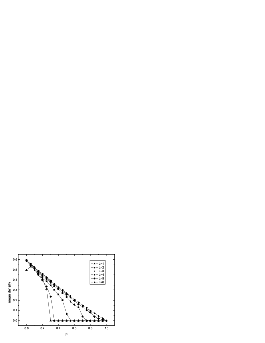
Figure 9: Mean density $\rho$ vs. $p$ for rule $18$ evolving under the third self-synchronization method. The existence of a transition to a synchronized state can be observed despite of the randomness in the election of neighbors within a range $L$, up to $L=4$.

4.2 Second Self-Synchronization Method

Now we introduce a new stochastic element in the application of the operator $\Gamma_{p}$. To differentiate from the previous case we call it $\tilde{\Gamma}_{\tilde{p}}$. The action of this operator consists in applying at each time the operator $\Gamma_{p}$, with $p$ chosen at random in the interval $(0,\tilde{p})$. The evolution law of the automaton is in this case:

$$\sigma(t+1)=\tilde{\Gamma}_{\tilde{p}}[(\sigma^{1}(t),\sigma^{2}(t))]=\tilde{\Gamma}_{\tilde{p}}[(\sigma(t),\Phi[\sigma(t)])].$$ (12)

The DA density between the present state and the previous one, defined as $\delta(t)=\mid\sigma(t)-\sigma(t-1)\mid$, is plotted as a function of $\tilde{p}$ for different rules $\Phi$ in Fig. 8. Only when the system becomes self-synchronized there will be a fall to zero in the DA density. Let us observe again that the behavior reported in the first self-synchronization method is newly obtained in this case. Rule $18$ undergoes a phase transition for a critical value of $\tilde{p}$. For $\tilde{p}$ greater than the critical value, the method is able to find the stable structure of the system (Sanchez & Lopez-Ruiz,, 2006). For the rest of the rules the freezing phase is not found. The dynamics generates patterns where the different marginally stable structures randomly compete. Hence the DA density decays linearly with $\tilde{p}$ (see Fig. 8).

Figure 10: Mean density $\rho$ vs. $p$ for different rules evolving under the third self-synchronization method. The density of the system decreases linearly with $p$.

4.3 Third Self-Synchronization Method

At last, we introduce another type of stochastic element in the application of the rule $\Phi$. Given an integer number $L$, the surrounding of site $i$ at each time step is redefined. A site $i_{l}$ is randomly chosen among the $L$ neighbors of site $i$ to the left, $(i-L,\ldots,i-1)$. Analogously, a site $i_{r}$ is randomly chosen among the $L$ neighbors of site $i$ to the right, $(i+1,\ldots,i+L)$. The rule $\Phi$ is now applied on the site $i$ using the triplet $(i_{l},i,i_{r})$ instead of the usual nearest neighbors of the site. This new version of the rule is called $\Phi_{L}$, being $\Phi_{L=1}=\Phi$. Later the operator $\Gamma_{p}$ acts in identical way as in the first method. Therefore, the dynamical evolution law is:

$$\sigma(t+1)=\Gamma_{p}[(\sigma^{1}(t),\sigma^{2}(t))]=\Gamma_{p}[(\sigma(t),\Phi_{L}[\sigma(t)])].$$ (13)

The DA density as a function of $p$ is plotted in Fig. 9 for the rule $18$ and in Fig. 10 for other rules. It can be observed again that the rule $18$ is a singular case that, even for different $L$, maintains the memory and continues to self-synchronize. It means that the influence of the rule is even more important than the randomness in the election of the surrounding sites. The system self-synchronizes and decays to the corresponding stable structure. Contrary, for the rest of the rules, the DA density decreases linearly with $p$ even for $L=1$ as shown in Fig. 10. The systems oscillate randomly among their different marginally stable structures as in the previous methods (Sanchez & Lopez-Ruiz,, 2006).

5 Symmetry Pattern Transition in Cellular Automata with Complex Behavior

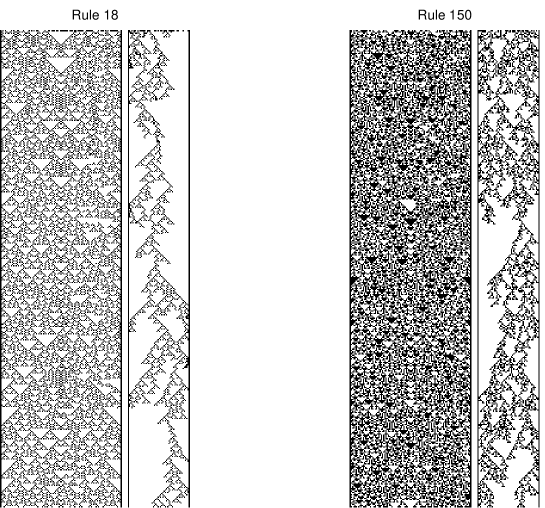
Figure 11: Space-time configurations of automata with $N=100$ sites iterated during $T=400$ time steps evolving under rules 18 and 150 for $p\lesssim p_{c}$. Left panels show the automaton evolution in time (increasing from top to bottom) and the right panels display the evolution of the corresponding DA.

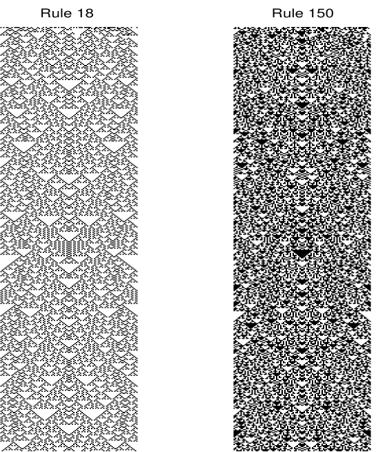
Figure 12: Time configurations of automata with $N=100$ sites iterated during $T=400$ time steps evolving under rules 18 and 150 using $p>p_{c}$. The space symmetry of the evolving patterns is clearly visible.

In this section, the stochastic synchronization method introduced in the former sections (Morelli & Zanette,, 1998) for two CA is specifically used to find symmetrical patterns in the evolution of a single automaton. To achieve this goal the stochastic operator, below described, is applied to sites symmetrically located from the center of the lattice. It is shown that a symmetry transition take place in the spatio-temporal pattern. The transition forces the automaton to evolve toward complex patterns that have mirror symmetry respect to the central axe of the pattern. In consequence, this synchronization method can also be interpreted as a control technique for stabilizing complex symmetrical patterns.

Cellular automata are extended systems, in our case one-dimensional strings composed of $N$ sites or cells. Each site is labeled by an index $i=1,\ldots,N$, with a local variable $s_{i}$ carrying a binary value, either $0$ or $1$. The set of sites values at time $t$ represents a configuration (state or pattern) $\sigma_{t}$ of the automaton. During the automaton evolution, a new configuration $\sigma_{t+1}$ at time $t+1$ is obtained by the application of a rule or operator $\Phi$ to the present configuration (see former section):

$$\sigma_{t+1}=\Phi\>[\sigma_{t}]\>.$$ (14)

5.1 Self-Synchronization Method by Symmetry

Our present interest (Sanchez & Lopez-Ruiz,, 2008) resides in those CA evolving under rules capable to show asymptotic complex behavior (rules of class III and IV). The technique applied here is similar to the synchronization scheme introduced by Morelli and Zanette (Morelli & Zanette,, 1998) for two CA evolving under the same rule $\Phi$. The strategy supposes that the two systems have a partial knowledge one about each the other. At each time step and after the application of the rule $\Phi$, both systems compare their present configurations $\Phi[\sigma^{1}_{t}]$ and $\Phi[\sigma^{2}_{t}]$ along all their extension and they synchronize a percentage $p$ of the total of their different sites. The location of the percentage $p$ of sites that are going to be put equal is decided at random and, for this reason, it is said to be an stochastic synchronization. If we call this stochastic operator $\Gamma_{p}$, its action over the couple $(\Phi[\sigma^{1}_{t}],\Phi[\sigma^{2}_{t}])$ can be represented by the expression:

$$(\sigma^{1}_{t+1},\sigma^{2}_{t+1})=\Gamma_{p}(\Phi[\sigma^{1}_{t}],\Phi[\sigma^{2}_{t}])=(\Gamma_{p}\circ\Phi)(\sigma^{1}_{t},\sigma^{2}_{t}).$$ (15)

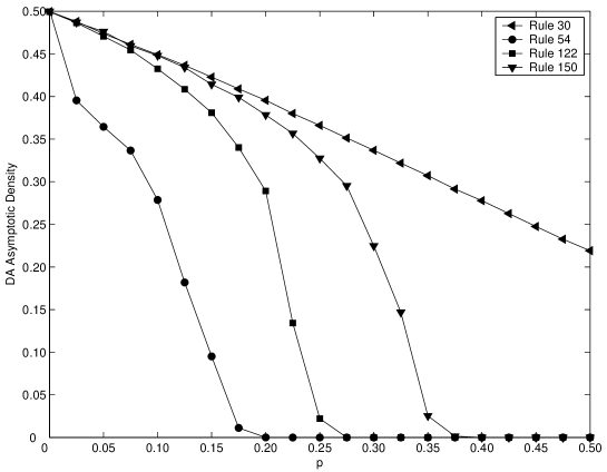
Figure 13: Asymptotic density of the DA for different rules is plotted as a function of the coupling probability $p$. Different values of $p_{c}$ for each rule appear clearly at the points where $\rho\to 0$. The automata with $N=4000$ sites were iterated during $T=500$ time steps. The mean values of the last $100$ steps were used for density calculations.

The same strategy can be applied to a single automaton with a even number of sites (Sanchez & Lopez-Ruiz,, 2008). Now the evolution equation, $\sigma_{t+1}=(\Gamma_{p}\circ\Phi)[\sigma_{t}]$, given by the successive action of the two operators $\Phi$ and $\Gamma_{p}$, can be applied to the configuration $\sigma_{t}$ as follows:

1. the deterministic operator $\Phi$ for the evolution of the automaton produces $\Phi[\sigma_{t}]$, and,

2. the stochastic operator $\Gamma_{p}$, produces the result $\Gamma_{p}(\Phi[\sigma_{t}])$, in such way that, if sites symmetrically located from the center are different, i.e. $s_{i}\neq s_{N-i+1}$, then $\Gamma_{p}$ equals $s_{N-i+1}$ to $s_{i}$ with probability $p$. $\Gamma_{p}$ leaves the sites unchanged with probability $1-p$.

Rule	$18$	$22$	$30$	$54$	$60$	$90$	$105$	$110$	$122$	$126$	$146$	$150$	$182$
$p_{c}$	$0.25$	$0.27$	$1.00$	$0.20$	$1.00$	$0.25$	$0.37$	$1.00$	$0.27$	$0.30$	$0.25$	$0.37$	$0.25$

Table 1: Numerically obtained values of the critical probability $p_{c}$ for different rules displaying complex behavior. Rules that can not sustain symmetric patterns need fully coupling of the symmetric sites, i.e. ($p_{c}=1$).

A simple way to visualize the transition to a symmetric pattern can be done by splitting the automaton in two subsystems ($\sigma^{1}_{t},\sigma^{2}_{t}$),

• $\sigma^{1}_{t}$, composed by the set of sites $s(i)$ with $i=1,\ldots,N/2$ and

• $\sigma^{2}_{t}$, composed the set of symmetrically located sites $s(N-i+1)$ with $i=1,\ldots,N/2$,

and displaying the evolution of the difference automaton (DA), defined as

$$\delta^{t}=\mid\sigma_{t}^{1}-\sigma_{t}^{2}\mid\>.$$ (16)

The mean density of active sites for the difference automaton, defined as

$$\rho^{t}={2\over N}\sum_{i=1}^{N/2}\delta^{t}$$ (17)

represents the Hamming distance between the sets $\sigma^{1}$ and $\sigma^{2}$. It is clear that the automaton will display a symmetric pattern when $\lim_{t\rightarrow\infty}\rho^{t}=0$. For class III and IV rules, a symmetry transition controlled by the parameter $p$ is found. The transition is characterized by the DA behavior:

when $$p<p_{c} \rightarrow \>\lim_{t\to\infty}\rho^{t}\neq 0$$ (complex non-symmetric patterns),

when $$p>p_{c} \rightarrow \hbox{$\>\lim_{t\to\infty}\rho^{t}=0$ (complex symmetric patterns)}.$$

The critical value of the parameter $p_{c}$ signals the transition point.

In Fig. 11 the space-time configurations of automata evolving under rules 18 and 150 are shown for $p\lesssim p_{c}$. The automata are composed by $N=100$ sites and were iterated during $T=400$ time steps. Left panels show the automaton evolution in time (increasing from top to bottom) and the right panels display the evolution of the corresponding DA. For $p\lesssim p_{c}$, complex structures can be observed in the evolution of the DA. As $p$ approaches its critical value $p_{c}$, the evolution of the DA become more stumped and reminds the problem of structures trying to percolate the plane (Pomeau,, 1986; Sanchez & Lopez-Ruiz, 2005-a, ). In Fig. 12 the space-time configurations of the same automata are displayed for $p>p_{c}$. Now, the space symmetry of the evolving patterns is clearly visible.

Table 1 shows the numerically obtained values of $p_{c}$ for different rules displaying complex behavior. It can be seen that some rules can not sustain symmetric patterns unless those patterns are forced to it by fully coupling the totality of the symmetric sites ($p_{c}=1$). The rules whose local dynamics verify $\phi(s_{1},s_{0},s_{2})=\phi(s_{2},s_{0},s_{1})$ can evidently sustain symmetric patterns, and these structures are induced for $p_{c}<1$ by the method here explained.

Finally, in Fig. 13 the asymptotic density of the DA, $\rho^{t}$ for $t\to\infty$, for different rules is plotted as a function of the coupling probability $p$. The values of $p_{c}$ for the different rules appear clearly at the points where $\rho\to 0$.

6 Conclusion

A method to measure statistical complexity in extended systems has been implemented. It has been applied to a transition to spatio-temporal complexity in a coupled map lattice and to a transition to synchronization in two stochastically coupled cellular automata (CA). The statistical indicator shows a peak just in the transition region, marking clearly the change of dynamical behavior in the extended system.

Inspired in stochastic synchronization methods for CA, different schemes for self-synchronization of a single automaton have also been proposed and analyzed. Self-synchronization of a single automaton can be interpreted as a strategy for searching and controlling the structures of the system that are constant in time. In general, it has been found that a competition among all such structures is established, and the system ends up oscillating randomly among them. However, rule $18$ is a unique position among all rules because, even with random election of the neighbors sites, the automaton is able to reach the configuration constant in time.

Also a transition from asymmetric to symmetric patterns in time-dependent extended systems has been described. It has been shown that one dimensional cellular automata, started from fully random initial conditions, can be forced to evolve into complex symmetrical patterns by stochastically coupling a proportion $p$ of pairs of sites located at equal distance from the center of the lattice. A nontrivial critical value of $p$ must be surpassed in order to obtain symmetrical patterns during the evolution. This strategy could be used as an alternative to classify the cellular automata rules -with complex behavior- between those that support time-dependent symmetric patterns and those which do not support such kind of patterns.

References

- Anteneodo & Plastino, (1996) Anteneodo, C. & Plastino, A.R. (1996). Some features of the statistical LMC complexity. Phys. Lett. A, Vol. 223, No. 5, 348-354.
- Argentina & Coullet, (1997) Argentina, M. & Coullet, P. (1997). Chaotic nucleation of metastable domains. Phys. Rev. E, Vol. 56, No. 3, R2359-R2362.
- Bennett, (1985) Bennett, C.H. (1985). Information, dissipation, and the definition of organization. In: Emerging Syntheses in Science, David Pines, (Ed.), 297-313, Santa Fe Institute, Santa Fe.
- Boccaletti et al., (2002) Boccaletti, S.; Kurths, J.; Osipov, G.; Valladares, D.L. & Zhou, C.S. (2002). The synchronization of chaotic systems. Phys. Rep., Vol. 366, No. 1-2, 1-101.
- Calbet & Lopez-Ruiz, (2001) Calbet, X. & López-Ruiz, R. (2001). Tendency toward maximum complexity in a non-equilibrium isolated system. Phys. Rev. E, Vol. 63, No.6, 066116(9).
- Chaitin, (1966) Chaitin, G. (1966). On the length of programs for computing finite binary sequences. J. Assoc. Comput. Mach., Vol. 13, No.4, 547-569.
- Chate & Manneville, (1987) Chaté, H. & Manneville, P. (1987). Transition to turbulence via spatio-temporal intermittency. Phys. Rev. Lett., Vol. 58, No. 2, 112-115.
- Cruthfield, (1989) Crutchfield, J.P. & Young, K. (1989) Inferring statistical complexity. Phys. Rev. Lett., Vol. 63, No. 2, 105-108.
- Feldman & Crutchfield, (1998) Feldman D.P. & Crutchfield, J.P. (1998). Measures of statistical complexity: Why?. Phys. Lett. A, Vol. 238, No. 4-5, 244-252.
- Grassberger, (1986) Grassberger, P. (1986). Toward a quantitative theory of self-generated complexity. Int. J. Theor. Phys., Vol. 25, No. 9, 907-915.
- Hawking, (2000) Hawking, S. (2000). “I think the next century will be the century of complexity”, In San José Mercury News, Morning Final Edition, January 23.
- Houlrik, (1990) Houlrik, J.M.; Webman, I. & Jensen, M.H. (1990). Mean-field theory and critical behavior of coupled map lattices. Phys. Rev. A, Vol. 41, No. 8, 4210-4222.
- Ilachinski, (2001) Ilachinski, A. (2001). Cellular Automata: A Discrete Universe, World Scientific, Inc. River Edge, NJ.
- Kaneko, (1989) Kaneko, K. (1989). Chaotic but regular posi-nega switch among coded attractors by cluster-size variation. Phys. Rev. Lett., Vol. 63, No. 3, 219-223.
- Kolmogorov, (1965) Kolmogorov, A.N. (1965). Three approaches to the definition of quantity of information. Probl. Inform. Theory, Vol. 1, No. 1, 3-11.
- Lamberti et al., (2004) Lamberti, W.; Martin, M.T.; Plastino, A. & Rosso, O.A. (2004). Intensive entropic non-triviality measure. Physica A, Vol. 334, No. 1-2, 119-131.
- Lempel & Ziv, (1976) Lempel, A. & Ziv, J. (1976). On the complexity of finite sequences. IEEE Trans. Inform. Theory, Vol. 22, 75-81.
- Lin, (1991) Lin, J. (1991). Divergence measures based on the Shannon entropy. IEEE Trans. Inform. Theory, Vol. 37, No. 1, 145-151.
- Lloyd & Pagels, (1988) Lloyd, S. & Pagels, H. (1988). Complexity as thermodynamic depth. Ann. Phys. (NY), Vol. 188, No. 1, 186-213.
- Lopez-Ruiz & Perez-Garcia, (1991) López-Ruiz, R. & Pérez-Garcia, C. (1991). Dynamics of maps with a global multiplicative coupling. Chaos, Solitons and Fractals, Vol. 1, No. 6, 511-528.
- Lopez-Ruiz, (1994) López-Ruiz, R. (1994). On Instabilities and Complexity, Ph. D. Thesis, Universidad de Navarra, Pamplona, Spain.
- Lopez-Ruiz et al., (1995) López-Ruiz, R.; Mancini, H.L. & Calbet, X. (1995). A statistical measure of complexity. Phys. Lett. A, Vol. 209, No. 5-6, 321-326.
- Lopez-Ruiz & Fournier-Prunaret, (2004) López-Ruiz, R. & Fournier-Prunaret, D. (2004). Complex behaviour in a discrete logistic model for the simbiotic interaction of two species. Math. Biosc. Eng., Vol. 1, No. 2, 307-324.
- Lopez-Ruiz, (2005) López-Ruiz, R. (2005). Shannon information, LMC complexity and Rényi entropies: a straightforward approach. Biophys. Chem., Vol. 115, No. 2-3, 215-218.
- Lovallo et al., (2005) Lovallo, M.; Lapenna, V. & Telesca, L. (2005) Transition matrix analysis of earthquake magnitude sequences. Chaos, Solitons and Fractals, Vol. 24, No. 1, 33-43.
- Martin et al., (2003) Martin, M.T.; Plastino, A. & Rosso, O.A. (2003). Statistical complexity and disequilibrium. Phys. Lett. A, Vol. 311, No. 2-3, 126-132.
- McKay, (2004) McKay, C.P. (2004). What is life?. PLOS Biology, Vol. 2, Vol. 9, 1260-1263.
- Menon et al., (2003) Menon, G.I.; Sinha, S. & Ray, P. (2003). Persistence at the onset of spatio-temporal intermittency in coupled map lattices. Europhys. Lett., Vol. 61, No. 1, 27-33.
- Morelli & Zanette, (1998) Morelli, L.G. & Zanette, D.H. (1998). Synchronization of stochastically coupled cellular automata. Phys. Rev. E, Vol. 58, No. 1, R8-R11.
- Perakh, (2004) Perakh, M. (2004). Defining complexity. In online site: On Talk Reason, paper: www.talkreason.org/articles/complexity.pdf.
- Pomeau & Manneville, (1980) Pomeau, Y. & Manneville, P. (1980). Intermittent transition to turbulence in dissipative dynamical systems. Commun. Math. Phys., Vol. 74, No.2, 189-197.
- Pomeau, (1986) Pomeau, Y. (1986). Front motion, metastability and subcritical bifurcations in hydrodynamics. Physica D, Vol. 23, No. 1-3, 3-11.
- Rolf et al., (1998) Rolf, J.; Bohr, T. & Jensen, M.H. (1998). Directed percolation universality in asynchronous evolution of spatiotemporal intermittency. Phys. Rev. E, Vol. 57, No. 3, R2503-R2506 (1998).
- Rosso et al., (2003) Rosso, O.A.; Martín, M.T. & Plastino, A. (2003). Tsallis non-extensivity and complexity measures. Physica A, Vol. 320, 497-511.
- Rosso et al., (2005) Rosso, O.A.; Martín, M.T. & Plastino, A. (2005). Evidence of self-organization in brain electrical activity using wavelet-based informational tools. Physica A, Vol. 347, 444-464.
- (36) Sánchez, J.R. & López-Ruiz, R., a, (2005). A method to discern complexity in two-dimensional patterns generated by coupled map lattices. Physica A, Vol. 355, No. 2-4, 633-640.
- (37) Sánchez, J.R. & López-Ruiz, R., b, (2005). Detecting synchronization in spatially extended discrete systems by complexity measurements. Discrete Dyn. Nat. Soc., Vol. 2005, No. 3, 337-342.
- Sanchez & Lopez-Ruiz, (2006) Sánchez, J.R. & López-Ruiz, R. (2006). Self-synchronization of Cellular Automata: an attempt to control patterns. Lect. Notes Comp. Sci., Vol. 3993, No. 3, 353-359.
- Sanchez & Lopez-Ruiz, (2008) Sánchez, J.R. & López-Ruiz, R. (2008). Symmetry pattern transition in Cellular Automata with complex behavior. Chaos, Solitons and Fractals, vol. 37, No. 3, 638-642.
- Shiner et al., (1999) Shiner, J.S.; Davison, M. & Landsberg, P.T. (1999). Simple measure for complexity. Phys. Rev. E, Vol. 59, No. 2, 1459-1464.
- Toffoli & Margolus, (1987) Toffoli, T. & Margolus, N. (1987). Cellular Automata Machines: A New Environment for Modeling, The MIT Press, Cambridge, Massachusetts.
- Wolfram, (1983) Wolfram, S. (1983). Statistical mechanics of cellular automata. Rev. Mod. Phys., Vol. 55, No. 3, 601-644.
- Yu & Chen, (2000) Yu, Z. & Chen, G. (2000). Rescaled range and transition matrix analysis of DNA sequences. Comm. Theor. Phys. (Beijing China), Vol. 33, No. 4, 673-678.
- Zimmermann et al., (2000) Zimmermann, M.G.; Toral, R.; Piro, O. & San Miguel, M. (2000). Stochastic spatiotemporal intermittency and noise-induced transition to an absorbing phase. Phys. Rev. Lett., Vol. 85, No. 17, 3612-3615.